Analytic solution of the Boltzmann equation in an expanding system
Abstract
For a massless gas with constant cross section in a homogeneous, isotropically expanding spacetime we reformulate the relativistic Boltzmann equation as a set of non-linear coupled moment equations. For a particular initial condition this set can be solved exactly, yielding the first analytical solution of the Boltzmann equation for an expanding system. The non-equilibrium behavior of this relativistic gas can be mapped onto that of a homogeneous, static non-relativistic gas of Maxwell molecules.
Keywords:
Relativistic Boltzmann equation, thermalization, analytical solutions, expanding systems.pacs
25.75-q,51.10.+y,52.27.Ny,98.80.-k1. Introduction. The relativistic Boltzmann equation plays a prominent role in understanding the complex non-equilibrium dynamics displayed by dilute relativistic gases. It has applications in many areas of physics including, e.g., theoretical description of the quark-gluon plasma [1, 2, 3, 4, 5, 6], neutrino transport in supernovae [7, 8], and structure formation in cosmology [9, 10, 11]. While analytical solutions of the Boltzmann equation have been thoroughly studied for homogeneous systems [12, 13, 14], solutions for an expanding system remain to be found even in the non-relativistic regime.
In the relativistic regime, progress in this direction was made recently [15, 16, 17, 18, 19, 20, 21, 22] using the Anderson-Witting equation [23], an approximation of the Boltzmann equation that relies on the relaxation time approximation [24]. In this scheme, the nonlinear collision kernel of the Boltzmann equation is replaced by a linearized version that qualitatively describes the relaxation of the system to equilibrium on a microscopic time scale. These analyses served to improve our understanding of the domain of applicability of a number of extended hydrodynamic theories used in the description of rapidly expanding plasmas [15, 16, 17, 18, 19, 20], with focus on the description of ultrarelativistic heavy-ion collisions.
However, a complete description of dilute gases can only be achieved by solving the full Boltzmann equation. While this can be done numerically, simple yet physically motivated analytical solutions of the Boltzmann equation, if available, can lead to valuable insights into non-equilibrium phenomena. In this Letter we take a step in this direction and derive the first analytical solution of the full Boltzmann equation for an expanding dilute gas. This is done using the method of moments [25, 6] to calculate the nonlinear collision term of the relativistic Boltzmann equation for a massless gas with constant cross section in a homogeneous and isotropically expanding spacetime. The derived solution describes the expansion-driven deviation of the particles’ momentum distribution from local thermal equilibrium as a function of the system’s expansion rate. We note that the non-expanding limit of this solution, which describes the homogeneous relaxation of a relativistic gas towards equilibrium, is also new.
2. Boltzmann equation. We consider a homogeneous and isotropically expanding system of massless particles in a Friedmann-Lemaître-Robertson-Walker (FLRW) metric [26, 27] (the most general homogeneous and isotropic metric in flat space)
| (1) |
We note that in this paper we make the further restriction of zero global curvature. For a gas of massless particles, the energy density and the pressure are related as , and here the scale factor [27] is a free function that may be fixed by additional physics assumptions. For the FLRW metric the nonzero Christoffel symbols are and , where denote spatial indices, is the Hubble parameter, and , with being the determinant of the metric in (1). Even though the fluid flow of this system is locally static, , the expanding FLRW geometry induces a nonzero fluid expansion rate .
The dynamics of the single-particle distribution function, , is given by the relativistic Boltzmann equation in curved space [30, 28, 29, 18, 19]
| (2) |
Since the FLRW geometry is based on the assumptions of spatial homogeneity and isotropy, cannot depend on spatial position and must be locally isotropic in momentum, depending only on where for massless particles with . We therefore write from here on.
The symmetries of the FLRW metric strongly constrain the form of the energy-momentum tensor and particle 4-current of the matter. Due to local momentum isotropy the viscous shear-stress tensor and particle diffusion current vanish exactly. Further, the bulk viscous pressure is zero for massless particles. Therefore, the conserved currents always take their equilibrium form, and the time evolution of the energy and particle densities, and , is fully determined by the conservation laws
| (3) |
With initial condition , they are solved by and .
Even though the conserved currents and take the same form as in local thermal equilibrium, the system itself does not have to be in equilibrium. In fact, the local momentum distribution is driven away from its local equilibrium form by an amount proportional to the expansion rate of the FLRW geometry. However, this process happens without disturbing the spatial homogeneity and isotropy of the system and, consequently, there are no out-of-equilibrium corrections to the conserved currents. A similar behavior was found in [21, 22] in the context of the relaxation time approximation.
The contributions from the Christoffel symbols in Eq. (2) cancel exactly, and the equation reduces to
| (4) |
Ignoring quantum statistics, the collision term reads
| (5) |
where and is the transition rate. To make progress on evaluating (5) we make the simplifying assumption of isotropic scattering with energy-independent total cross section . Then takes the form [28, 29, 30]
| (6) |
where . Thus, the Boltzmann equation becomes
| (7) |
Note that even for the highly symmetric case considered here the relativistic Boltzmann equation is still a nonlinear integro-differential equation for .
3. Moment equations. We proceed to solve the Boltzmann equation using the method of moments [6]. Due to local momentum isotropy, the distribution function can be fully described by scalar moments only [31]:
| (8) | |||||
The time dependence of the two lowest moments, the number density and the energy density , is given by the conservation laws already discussed. For a classical gas of massless particles, they provide the time-dependence of the temperature and fugacity (where is the chemical potential) via the matching conditions [6] and where is the number of massless degrees of freedom (including statistical degeneracy factors). In the following we set for simplicity.
From the matching conditions it follows that and such that the fugacity is time-independent. and define the local equilibrium distribution function and the equilibrium scalar moments
| (9) |
To express the Boltzmann equation in terms of the scalar moments we multiply (7) by and integrate over . This results in
| (10) |
where the gain and loss terms are defined by
Here the gain term was simplified by using the symmetry of the transition rate under interchange of the incoming and outgoing momenta. With
| (12) |
the loss term reduces straightforwardly to [6]
| (13) |
However, the gain term is more involved. One first writes
| (14) |
where the inner kernel is
| (15) |
This quantity is a scalar and can be calculated in any frame. In the center of momentum frame, the 4-dimensional delta function can be integrated and the remaining angular integrals can be performed analytically [32]. The final result can be expressed as follows
| (16) |
Plugging this back into (14) and performing some algebraic manipulations [32] one obtains
| (17) |
Using these results in Eq. (10) we derive the following exact evolution equation for the moments:
| (18) |
This infinite set of coupled nonlinear differential equations for the scalar moments is equivalent to the original relativistic integro-differential Boltzmann equation. For and Eq. (18) reduces to Eqs. (3) for the particle and energy densities. Higher-order moments are more sensitive to the distribution function at higher momentum. We can further simplify the moment equations by introducing the scaled moments [33] and the scaled time where is the (constant) mean free path at time . This yields the surprisingly simple evolution equations
| (19) |
Equation (19) is the main result of this Letter. While the nonlinear coupling between different moments was expected from the nonlinearity of the collision kernel, the same cannot be said about another key feature of Eq. (19): it can be solved recursively, i.e. the solution of the evolution equation for requires only previously solved moments of lower order . This property depends on our choice of an energy-independent cross section; it is essential for being able to solve (19) analytically.
All information about the expansion appears in the factor multiplying the time derivative in (19). Whether or not local equilibrium can be achieved thus depends on the state of expansion of the system. For example, when the mean free path increases faster than the expansion rate, , and local equilibrium cannot be reached even at asymptotically large times. Moreover, if the initial is positive definite, , and Eq. (19) then implies that all moments remain positive throughout the evolution, translating into positivity for for all momenta at all times.
Equation (19) closely resembles the Bobylev-Krook-Wu (BKW) equation derived almost four decades ago [12, 13] in a famous study about homogeneous and isotropic solutions of the non-relativistic Boltzmann equation (for a review see [14]) for Maxwell molecules. In fact, by defining the time variable to take into account the expansion [34], our equation (19) for the moments becomes identical to the BKW equations [13]:
| (20) |
This indicates that even though the underlying symmetries of these physical systems are quite different (BKW’s are based on Galilean invariance with static conditions while ours are embedded in an expanding system), these systems are actually equivalent from a dynamical perspective and evolve towards equilibrium in a universal manner. We note that our equations also reduce to BKW’s when , i.e. for a non-expanding metric (though special relativistic effects are still fully taken into account).
4. Analytical solution of the moment equations. Given the close relation of our Eq. (19) with the BKW equation (20) it is not surprising that it admits an exact analytic solution of the Krook and Wu type:
| (21) |
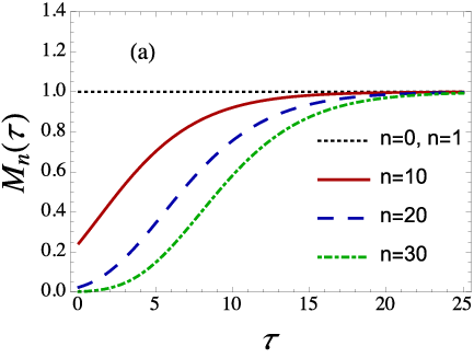
where . The time evolution of the moments is shown in Fig. 1 (a). One sees that low-order moments equilibrate more quickly than the higher-order ones that are needed to describe the high-momentum non-equilibrium tail of the distribution function.
Given the exact form (21) of the moments , the distribution function can be reconstructed as follows. One defines the function where , expands its Fourier transform with respect to in terms of the moments , and then transforms it back. This yields the exact result [32]
| (22) | |||||
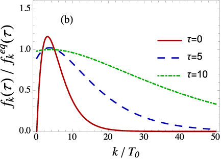
To the best of our knowledge, this is the first analytic solution of the full Boltzmann equation for an expanding interacting gas. At the initial time (corresponding to and ) one finds the initial condition . In Fig. 1 (b) we plot the analytical solution for the ratio as a function of for , , and . At the high momentum tail is largely underpopulated whereas momentum modes in the range are over-occupied relative to local equilibrium. As time evolves, high momentum modes are populated at the expense of the over-populated moderate momentum region, in a process resembling an energy cascade. Note, however, that when one finds that is finite and (22) never assumes the equilibrium form.
The moment equations (19) can also be studied numerically for a variety of initial conditions for which no analytic solution is known. Here we briefly address the question whether the direct energy cascade seen in Fig. 1 is related to self-similar behavior characteristic of turbulence [35]. While a detailed study of self-similarity in this system is beyond the scope of this short paper, we note here that expressing the Boltzmann equation in terms of its moments may be quite useful in this context. For instance, one can show that non-thermal fixed points corresponding to exact self-similar solutions of the kind
| (23) |
where and are the scaling exponents and is the fixed point distribution [35], are not compatible with Eq. (19). In fact, using Eq. (3) one can see that the scaling exponents are necessarily and , and that the Ansatz (23) for the distribution function (if assumed to be valid for all momenta) leads to moments
| (24) |
(where ) that have the same time dependence as the equilibrium moments. This implies that the corresponding normalized moments are time independent. Since the conservation laws require that , one can then use (19) to show that for all . This shows that there are no other true fixed points of the dynamics besides local thermal equilibrium.
6. Conclusions. We derived from the relativistic Boltzmann equation a nonlinear set of coupled moment equations for a massless gas with constant cross section in a homogeneous, isotropically expanding spacetime. For a particular initial condition, we found that the moment equations can be solved exactly, thereby obtaining the first analytical solution of the Boltzmann equation with full non-linear collision term for an expanding system.
The normalized moments of this expanding relativistic gas can be directly mapped onto the corresponding moments for a homogeneous, static non-relativistic gas of Maxwell molecules. This happens even though the distribution functions of these systems are not the same. This nontrivial correspondence suggests that exact self-similar non-equilibrium solutions may not exist even in rapidly expanding systems.
The study performed here can be extended along several directions. One may consider different types of cross sections, or include nonzero particle masses to investigate bulk viscous effects. If possible, the generalization of the method presented here to expanding systems with different symmetries [15, 18, 36, 37, 38] that are relevant for the study of the quark-gluon plasma formed in heavy ion collisions would be particularly desirable.
Acknowledgements. GSD thanks S. Schlichting and A. Dumitru for enlightening discussions. MM thanks Y. Mehtar-Tani and S. Ozonder for useful discussions. JN thanks the Physics Department at Columbia University for its hospitality and Conselho Nacional de Desenvolvimento Científico e Tecnológico (CNPq) and Fundação de Amparo à Pesquisa do Estado de São Paulo (FAPESP) for financial support. UH and MM express their gratitude to the Institute for Nuclear Theory for hospitality during the final stages of this work. GSD thanks the Kavli Institute of Theoretical Physics China (KITPC) for hospitality during the initial stages of this work. GSD is currently supported under DOE Contract No. DE-SC0012704 and acknowledges previous support of a Banting fellowship provided by the Natural Sciences and Engineering Research Council of Canada. DB, UH, and MM are supported by the U.S. Department of Energy, Office of Science, Office of Nuclear Physics under Award DE-SC0004286. UH, MM and JN gratefully acknowledge support through a bilateral travel grant from FAPESP and the Ohio State University.
References
- [1] U. Heinz, Annals Phys. 161, 48 (1985); 168, 148 (1986).
- [2] S. A. Bass et al., Prog. Part. Nucl. Phys. 41, 255 (1998).
- [3] P. B. Arnold, G. D. Moore and L. G. Yaffe, JHEP 0011, 001 (2000).
- [4] D. Molnar and M. Gyulassy, Nucl. Phys. A 697, 495 (2002) [Erratum: Nucl. Phys. A 703, 893 (2002)].
- [5] Z. Xu and C. Greiner, Phys. Rev. C 71, 064901 (2005).
- [6] G. S. Denicol, H. Niemi, E. Molnar and D. H. Rischke, Phys. Rev. D 85, 114047 (2012) [Erratum: Phys. Rev. D 91, 039902 (2015)].
- [7] M. Liebendoerfer, M. Rampp, H.-T. Janka and A. Mezzacappa, Astrophys. J. 620, 840 (2005).
- [8] H. T. Janka, K. Langanke, A. Marek, G. Martinez-Pinedo and B. Mueller, Phys. Rept. 442, 38 (2007).
- [9] C. P. Ma and E. Bertschinger, Astrophys. J. 455, 7 (1995).
- [10] S. Dodelson, Modern Cosmology (Academic Press, 2003).
- [11] S. Weinberg, Cosmology, (Oxford University Press, 2008).
- [12] A. V. Bobylev, Sov. Phys. Dokl. 20, 820 (1976).
- [13] M. Krook and T. T. Wu, Phys. Rev. Lett. 36,1107 (1976); Phys. Fluids 20, 1589 (1977).
- [14] M. H. Ernst, J. Stat. Phys. 34, 5/6 (1984).
- [15] W. Florkowski, R. Ryblewski and M. Strickland, Nucl. Phys. A 916, 249 (2013).
- [16] W. Florkowski, R. Ryblewski and M. Strickland, Phys. Rev. C 88, 024903 (2013).
- [17] G. S. Denicol, W. Florkowski, R. Ryblewski and M. Strickland, Phys. Rev. C 90, 044905 (2014).
- [18] G. S. Denicol, U. Heinz, M. Martinez, J. Noronha and M. Strickland, Phys. Rev. Lett. 113, 202301 (2014).
- [19] G. S. Denicol, U. Heinz, M. Martinez, J. Noronha and M. Strickland, Phys. Rev. D 90, 125026 (2014).
- [20] M. Nopoush, R. Ryblewski and M. Strickland, Phys. Rev. D 91, no. 4, 045007 (2015).
- [21] J. Noronha and G. S. Denicol, arXiv:1502.05892 [hep-ph].
- [22] Y. Hatta, M. Martinez and B. W. Xiao, Phys. Rev. D 91, 085024 (2015).
- [23] J. L. Anderson and H. R. Witting, Physica 74, 466 and 489 (1974).
- [24] P. L. Bhatnagar, E. P. Gross and M. Krook, Phys. Rev. 94, 511 (1954).
- [25] H. Grad. Commun. Pure Appl. Math. 2, 325.
- [26] S. Weinberg, Gravitation and Cosmology: Principles and Applications of the General Theory of Relativity (John Wiley & Sons, 1972).
- [27] D. Baumann, Cosmology Part III: Mathematical Tripos, avaliable at http://www.damtp.cam.ac.uk/user/db275/Cosmology/Lectures.pdf.
- [28] C. Cercignani and G. M. Kremer, The Relativistic Boltzmann Equation: Theory and Applications (Boston; Basel; Berlin: Birkhäuser, 2002).
- [29] J. Bernstein, Kinetic Theory in the Expanding Universe (Cambridge University Press, 1988).
- [30] F. Debbasch and W. van Leeuwen, Physica A 388,1079 and 1818 (2009).
- [31] For anisotropic systems, this is no longer true and one must consider additional irreducible moments of [6].
- [32] D. Bazow, G. S. Denicol, U. Heinz, M. Martinez, J. Noronha, in preparation.
- [33] Eqs. (3) and the matching conditions imply that throughout the evolution.
- [34] This is equivalent to scaling the time by the time-dependent mean free path instead of the constant used above Eq. (19).
- [35] J. Berges, arXiv:1503.02907 [hep-ph].
- [36] T. Epelbaum and F. Gelis, Phys. Rev. Lett. 111, 232301 (2013).
- [37] J. Berges, K. Boguslavski, S. Schlichting and R. Venugopalan, Phys. Rev. D 89, 114007 (2014).
- [38] A. Kurkela and Y. Zhu, Phys. Rev. Lett. 115, no. 18, 182301 (2015).