Distributed First Order LogicThanks: This paper is a substantially revised and extended version of a paper with the same title presented at the 1998 International Workshop on Frontiers of Combining Systems (FroCoS’98)

The magic box, together with the balls, represents a “complex” environment corresponding to the domain of the agents’ local knowledge bases. The agents’ points of view correspond to their local knowledge. The local knowledge of the agents is constrained one another by the fact that they describe views over the same environment. Assuming that we have a complete description of the box we can build the agents’ local knowledge (bases) as views over this complete description. However, such a complete description is often not available. What we often have are only the partial views, and a set of constraints between these views, with no representation of the external world (in our example case, the entire box). In cases like this we need a logical formalism able to describe the point of view of the different agents ($Mr.1$, and $Mr.2$, in our example) and the constraints among these views, without having to represent the entire box as we see it in Figure 1(a). The formalism should be able to represent and reason about statements such as:

1. 1.

   “the domain of $Mr.1$ contains 3 balls and a box with 2 sectors”;

2. 2.

   “$Mr.2$ sees a black ball in the right sector”;

3. 3.

   “$Mr.1$ and $Mr.2$ agree on the colour of the balls they both see”;

4. 4.

   “if $Mr.1$ sees an empty box, then $Mr.2$ sees an empty box too”;

5. 5.

   “if $Mr.2$ sees 3 balls in the box, then the leftmost is also seen by $Mr.1$”.

This example involves, in a very simple form, a number of crucial aspects of distributed knowledge representation: first, it deals with heterogeneous local domains which correspond to the different sets of balls in the different viewpoints. Second, it has to do with cross-domain identity. In fact, we need to represent the connections between the perceptions of the balls by each agent, without having an objective model that completely and correctly describes all the objects (balls) present in the box. An example is statement 5 above. Third, we have heterogeneous local properties. In our example $Mr.1$ sees a box composed of two sectors, while for $Mr.2$ the box is composed of three sectors. Thus $Mr.2$ has a a notion of “a ball being in the central sector” which $Mr.1$ does not have. Fourth, it deals with constrained viewpoints. The viewpoints of the agents are, in fact, not independent, since they are the result of they observing the the environment. Thus, if $Mr.1$ sees an empty box, then $Mr.2$ is constrained to see an empty box too, as described in statement 4 above.

Information integration is often based on architectures that make use of a mediator [72], as in the following example.

Even if we discard details on how the information is integrated, and the process of query-answering is performed, we can observe that a logic for the representation of such a scenario must be able to represent the heterogeneous schemata and domains of the three subsystems $m$, $\it Sel.1$, and $Sel.2$. In particular the formalism should be able to represent the following facts:

1. 1.

   $\it Sel.1$ sells “apples”, whereas $Sel.2$ and $m$ represent the domain of apples at a greater granularity, and are able to offer specific varieties of apples (ranging among Delicious and Granny Smith in our example). Moreover, for the sake of the example, the “apples” of $\it Sel.1$ correspond to both “Delicious” and “GrannySmith” in the mediator. This justifies the disjunctive statement retrieved by the mediator as a “translation” of the statements about apples contained in the database of $\it Sel.1$;

2. 2.

   total prices of $Sel.2$ are transformed in prices per kilo in $m$ to be homogeneous with price format of $\it Sel.1$;

3. 3.

   $m$ is not interested in retrieving information about fruits whose price is not yet defined (lemons in our case);

4. 4.

   the information goes from $\it Sel.1$ (resp. $Sel.2$) to $m$ and not from the mediator to the sellers.

Again, this example involves heterogeneous local domains and cross-domain identity, as described in statement 1 above. Moreover, it involves heterogeneous local properties represented by the different relations, which are nonetheless constrained by the fact that they all represent the availability of fruit at a certain price. Thus, for example, if 10 Kg of oranges cost 20 Euros in the database of $Sel.2$, then oranges cost 2 Euros per Kilo in the database of the mediator. In addition, information is required to be directional: in our example it flows from the sellers to the mediator and not vice-versa, since the sellers must be prevented to retrieve knowledge about potential competitors that could be stored in the mediator.

Let $\{L_{i}\}_{i\in I}$ (hereafter $\{L_{i}\}$) be a family of first-order languages defined over a non empty set $I$ of indexes. For the sake of simplicity we assume, without loss of generality, that all the languages $L_{i}$ contain the same set $X$ of infinitely many variables. Each language $L_{i}$ is the language used by the $i$-th local knowledge base to partially describe the world from its own perspective. For instance, in the magic box example $I=\{1,2\}$.

In DFOL, each $L_{i}$ is a first-order language with equality, extended with a new set of symbols, called arrow variables, which are of the same syntactic type as constants and standard individual variables (hereafter often called non-arrow variables). Formally, for each variable $x\in X$, and each index $i,j\in I$, with $i\neq j$, the signature of $L_{i}$ is extended to contain the two arrow variables $\overset{\rightarrow j}{\negthickspace x}$ and $\overset{j\rightarrow}{x}$.

The arrow variables $\overset{\rightarrow j}{\negthickspace x}$ and $\overset{j\rightarrow}{x}$ in $L_{i}$ intuitively denote an object in the domain of interpretation of $L_{i}$ that corresponds to the object $x$ in the domain of $L_{j}$. The difference between $\overset{\rightarrow j}{\negthickspace x}$ and $\overset{j\rightarrow}{x}$ will become clearer later in the paper. We often use $\overset{\rightarrow}{x}$ to denote a generic arrow variable (that is, either of the form $\overset{\rightarrow j}{\negthickspace x}$ or $\overset{j\rightarrow}{x}$).

Terms of $L_{i}$, also called $i$-terms, are recursively defined as in first-order logic starting from the set of constants, variables, and arrow variables, and by recursively applying function symbols. Formally:

1. 1.

   Any constant, variable, and arrow variable of $L_{i}$ is a $i$-term.

2. 2.

   If $f$ is a function symbol of arity $n$ in $L_{i}$ and $t_{1},\ldots,t_{n}$ are $i$-terms, then $f(t_{1},...,t_{n})$ is a $i$-term.

Formulas of $L_{i}$, called $i$-formulas, are defined as in first-order logic, with the discriminant that we only quantify over non-arrow variables. Formally:

1. 1.

   If $P$ is a n-ary predicate symbol in $L_{i}$ and $t_{1},\ldots,t_{n}$ are $i$-terms, then $P(t_{1},...,t_{n})$ is a $i$-formula.

2. 2.

   If $t_{1}$ and $t_{2}$ are $i$-terms, then $t_{1}=t_{2}$ is a $i$-formula.

3. 3.

   If $\phi$ and $\psi$ are $i$-formulas, then $\lnot\phi$, $\phi\supset\psi$, $\phi\wedge\psi$, $\phi\vee\psi$, are $i$-formulas.

4. 4.

   If $\phi$ is a formula and $x$ is a non-arrow variable, then $\forall x\phi$ and $\exists x\phi$ are $i$-formulas.

Examples of $i$-terms are $x$, $c$, $\overset{\rightarrow j}{\negthickspace x}$, $f(c,d)$, and $f(\overset{j\rightarrow}{x},f(g(d)))$. Examples of $i$-formulas are $P(x,y,z)$, $P(\overset{\rightarrow j}{\negthickspace x},w,a)$, $\bot\supset P(f(c),d)$, $\forall x.P(x,y)$, $\forall x.x=\overset{j\rightarrow}{x}$, $\exists y.P(y,\overset{\rightarrow j}{\negthickspace x})$. Instead $\forall\overset{j\rightarrow}{x}.P(\overset{j\rightarrow}{x})$ is not an $i$-formula as we do not allow quantification on arrow variables.

A $i$-formula $\phi$ is closed if it does not contain arrow variables and all the occurrences of the variable $x$ in $\phi$ are in the scope of a quantifier $\forall x$ or $\exists x$. $\phi$ is open if it is not closed. A variable $x$ occurs free in a formula if $x$ occurs in $\phi$ not in the scope of a quantifier $\forall x$ or $\exists x$. Notice that $x$, $\overset{\rightarrow i}{\negthickspace x}$ and $\overset{i\rightarrow}{x}$ are different variables, and therefore $x$ does not occur free in an expression of type $p(\overset{\rightarrow i}{\negthickspace x})$. The notation $\phi({\bf x})$ is used to denote the formula $\phi$ and the fact that the free variables of $\phi$ are ${\bf x}=\{x_{1},\ldots,x_{n}\}$.

Languages $L_{i}$ and $L_{j}$ are not necessarily disjoint and the same formula $\phi$ can occur in different languages with different meanings. A labeled formula is a pair $i\!:\!\phi$³³ 3 Similar notations are introduced in [54, 24, 71, 20, 52]. and is used to denote that $\phi$ is a formula in $L_{i}$. Given a set of $i$-formulas $\Gamma$, we use $i\!:\!\Gamma$ as a shorthand for the set of labelled formulas $\{i\!:\!\gamma|\gamma\in\Gamma\}$. Note that we do not admit formulas which are composed of symbols coming from different alphabets. Thus $1\!:\!P(x)\wedge 2\!:\!a=b$ and $\forall x1\!:\!P(x)$ are not well-formed labeled formulas in DFOL.

DFOL associates different domains of interpretation to the local knowledge bases; therefore it needs a mechanism to denote cross-domain identity. Arrow variables provide such a mechanism, and are used to refer to counterpart objects which belong to other domains. In particular, arrow variables of the form $\overset{j\rightarrow}{x}$ and $\overset{\rightarrow j}{\negthickspace x}$ occurring in a $i$-formula are used to denote an object in the domain of interpretation of $L_{i}$, which corresponds to the object denoted by $x$ in the domain of $L_{j}$.

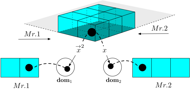
Consider, for instance, statement 3 at page 3. The formalisation of this statement requires the ability to represent a ball that is seen by both observers. Since DFOL represents the partial viewpoints of $Mr.1$ and $Mr.2$, each one with its own domain of interpretation, there is no object that directly represents a ball seen by both. Indeed, consider the black ball in the corner of the magic box represented at the top of Figure 3. $Mr.1$ and $Mr.2$ have their own representation of this ball in their different domains, as graphically depicted at the bottom of Figure 3. The way we represent the connection between these two different objects is by using an arrow variable, say $\overset{\rightarrow 2}{\negthickspace x}$, interpreted in the domain of $Mr.1$ which corresponds to the ball denoted by $x$ seen by $Mr.2$. We can then predicate that both $\overset{\rightarrow 2}{\negthickspace x}$ and $x$ are black using the formulas $1\!:\!\textit{black}(\overset{\rightarrow 2}{\negthickspace x})$ and $2\!:\!\textit{black}(x)$. The precise way in which DFOL binds the interpretation of $\overset{\rightarrow 2}{\negthickspace x}$ and $x$ in the different domains will become clear with the definition of Assignment (Definition 4).

The notion of arrow variable introduced here is connected to the notion of counterparts introduced by Lewis in [48]. Roughly speaking, the language of Lewis’ Counterpart Theory contains a binary predicate $C(x,y)$ meaning that $x$ is the counterpart of $y$, where $x$ and $y$ are supposed to denote two objects in two different possible worlds. In DFOL, we have local knowledge bases with different local languages instead of possible worlds. Therefore, we cannot explicitly state that $x$ is counterpart of $y$, when $x$ and $y$ belong to two different languages, but only state it implicitly by means of arrow variables. That is, we can name in the language $L_{i}$ a counterpart of $x$ in $L_{j}$ by using the arrow variables $\overset{j\rightarrow}{x}$ and $\overset{\rightarrow j}{\negthickspace x}$.

The semantics of a family of DFOL languages $\{L_{i}\}$ is defined by associating a set of interpretations, called local models, to each $L_{i}$ in $\{L_{i}\}$ and by relating objects in different domains via, so-called, domain relations. This semantics is an extension of Local Models Semantics as defined in [28]. If we look at the knowledge contained in a knowledge base $i$ we can distinguish three cases. First, $i$ can be complete, that is, for each formula $\phi\in L_{i}$ either $\phi$ or $\neg\phi$ belongs to the (deductive closure of the) knowledge base; second, it can be incomplete, if there exist at least a formula $\phi$ such that neither $\phi$ or $\neg\phi$ belongs to it; third, it can be inconsistent, that is, both $\phi$ and $\neg\phi$ belong to it. To represent these three possible statuses, each $i$ is associated with a (possibly empty) set of local models. That is, each $i$ is associated with an epistemic state. A singleton corresponds to a complete KB, the empty set corresponds to an inconsistent KB, whereas all the other sets correspond to an incomplete KB. While completeness w.r.t. the entire language $L_{i}$ may be unrealistic, and even undesirable, it may be a good property to require for certain types of formulas, as we will see in the following paragraphs. To characterise the portion of knowledge upon which $i$ has complete knowledge we introduce the notion of complete sub-language $L_{i}^{c}$ and we restrict the definition of complete knowledge to the formulas of $L_{i}^{c}$. Let $L_{i}^{c}$ be a sub-language of $L_{i}$ built from a subset of constants, functional symbols, and predicate symbols of $L_{i}$, including equality, plus the set of arrow and not-arrow variables of $L_{i}$. We call $L_{i}^{c}$ the complete sub-language of $L_{i}$. Complete terms and complete formulas are terms and formulas of $L_{i}^{c}$. Otherwise they are called non complete. Note that in DFOL $L_{i}^{c}$ must contain the equality predicate as we impose that each $i$-th knowledge base is able to evaluate whether two objects are equal or not. Additional constants, functional symbols, or predicates can be added to $L_{i}^{c}$ to represent domain-specific complete knowledge. For instance, in the magic box example we may assume that $Mr.1$ and $Mr.2$ have complete knowledge about the position of the balls. That is, they know if a ball is in a slot or not. On the contrary, assume that $Mr.2$’s view over the box is partially concealed by a big wall, as depicted in Figure 4. In this scenario $Mr.2$ is able to see one box sector and knows that there are two sectors behind the wall with balls inside and outside the box. In this case $Mr.2$ has complete knowledge about the left hand side position of the box but is uncommitted to whether there are balls in the sectors behind the wall. This is formalised by including the formulas $inbox(b,l)$ into $L_{2}^{c}$ for all the balls $b$ in the language of $Mr.2$, and by letting, e.g., sentences of the form $inbox(b,c)$ to be non complete, that is, true in some local model of $Mr.2$ and false in others.

The semantic overlap between different knowledge bases is explicitly represented in DFOL by means of domain relations.

We often use the simpler expression domain relation from $i$ to $j$ to denote a domain relation $r_{ij}$ from ${\bf dom}_{i}$ to ${\bf dom}_{j}$. We also use the functional notation ${r}_{ij}(d)$ to denote the set $\{d^{\prime}\in{\bf dom}_{j}|\langle d,d^{\prime}\rangle\in{r}_{ij}\}$.

A domain relation from $i$ to $j$ illustrates how the $j$-th knowledge base represents the domain of the $i$-th knowledge base in its own domain. Therefore, a pair $\langle d,d^{\prime}\rangle$ being in ${r}_{ij}$ means that, from the point of view of $j$, $d$ in ${\bf dom}_{i}$ is the representation of $d^{\prime}$ in ${\bf dom}_{j}$. Thus, ${r}_{ij}$ formalises $j$’s subjective point of view on the relation between ${\bf dom}_{i}$ and ${\bf dom}_{j}$, and not an absolute and objective point of view; this implies that $\langle d,d^{\prime}\rangle\in{r}_{ij}$ must not be read as if $d$ and $d^{\prime}$ were the same object in a domain shared by $i$ and $j$. This latter fact could only be formalised by an external (above, meta) observer to both $i$ and $j$.

Domain relations are not symmetric by default. This represents the fact that the point of view of $j$ over the domain of $i$ may differ from the point of view of $i$ over the domain of $j$, which may even not exist. For instance, in the mediator system example, it is plausible to impose that $m$ has a representation of the domains of $\it Sel.1$ and $Sel.2$, in its own domain while the opposite is prevented. Domain relations are conceptually analogous to conversion functions between semantic objects, as defined in [64].

Specific relations between the domains of different knowledge bases can be modelled by adding constraints about the form of ${r}_{ij}$. For instance, two knowledge bases with different but isomorphic representations of the same domain can be modelled by imposing ${r}_{ij}={r}^{-1}_{ji}$. Likewise, completely unrelated domains can be represented by imposing ${r}_{ij}={r}_{ji}=\emptyset$. Transitive mappings between the domains of three knowledge bases $i$, $j$ and $k$ can be represented by imposing ${r}_{ik}={r}_{ij}\circ{r}_{jk}$. Moreover, if ${\bf dom}_{i}$ and ${\bf dom}_{j}$ are ordered according to two ordering relations $<_{i}$ and $<_{j}$ respectively, then a domain relation that satisfies the following property

formalises a mapping which preserves the ordering. An example of this last property is a domain relation that captures a currency exchange function. Further constraints on ${r}_{ij}$ are discussed in Section 4.

The definition above extends the classical notion of assignment given for first-order logic to deal with extended variables. Intuitively, if the non-arrow variable $x$ occurring in the $j$-th knowledge base is a placeholder for the element $d\in{\bf dom}_{j}$, then the occurrence of the arrow variable $\overset{\rightarrow j}{\negthickspace x}$ in a formula of the $i$-th knowledge base is a placeholder for an element $d^{\prime}\in{\bf dom}_{i}$ which is a pre-image (via ${r}_{ij}^{-1}$) of $d$. Analogously, the arrow variable $\overset{j\rightarrow}{x}$ occurring in $i\!:\!\psi$ is a placeholder for any element $d^{\prime\prime}\in{\bf dom}_{i}$ which is an image (via ${r}_{ji}$) of $d$.

An assignment $a^{\prime}$ is an extension of $a$, in symbols $a\leq a^{\prime}$, if $a_{i}(v)=d$ implies $a_{i}^{\prime}(v)=d$ for all the non-arrow and arrow variables $v$. Notationally, given an assignment $a$, a (non-arrow or arrow) variable $x$, and an element $d\in{\bf dom}_{i}$, we denote with $a(x:=d)$ the assignment obtained from $a$ by letting $a_{i}(x)=d$.

With an abuse of notation we use the symbol $\models$ of satisfiability to denote both first-order satisfiability and DFOL satisfiability. The context will always make clear the distinction between the two.

If we compare satisfiability of a formula in a DFOL model with the standard notion of satisfiability of a first-order formula in a first-order model we can observe three differences: first, assignments do not force all arrow variables to denote objects in the domain; second, we admit partial knowledge as we evaluate the satisfiability of a formula in a set of local models, rather than into a single one; third, we admit islands of inconsistency, by allowing some $M_{i}$ to be empty. In the following we analyse these three aspects one by one.

The DFOL language described so far is able to represent the different local KBs, but cannot be used to express formulas spanning over different knowledge bases. We enrich DFOL with this ability by introducing a class of “cross language formulas”. These formulas are an extension of the notion of bridge rule, first introduced in [32] in a proof-theoretic setting.

A bridge rule can be seen as an axiom spanning between different logical theories (the local knowledge bases); it restricts the set of possible DFOL models to those in which $i\!:\!\phi$ is a logical consequence of $i_{1}\!:\!\phi_{1},\dotsc,i_{n}\!:\!\phi_{n}$. We call $i_{1}\!:\!\phi_{1},\ldots,i_{n}\!:\!\phi_{n}$ the premises of the rule and $i\!:\!\phi$ the conclusion. As an example, the bridge rule

represents the fact that the rightmost ball seen by $Mr.1$ inside the box is seen also by $Mr.2$.

Given a set of bridge rules ${\sf BR}$ on the family of languages $\{L_{i}\}$, a ${\sf BR}$-model is a DFOL model for $\{L_{i}\}$ that satisfies all the bridge rules of ${\sf BR}$.

Definition 8 enables us to illustrate the difference between $i\!:\!\phi\supset\psi$ and $i\!:\!\phi\rightarrow i\!:\!\psi$. Let us disregard here the requirement of the existence of $a^{\prime}$ extension of $a$. ${\cal{M}}\models i\!:\!\phi\supset\psi$ is satisfied if all local models $m_{i}\in{\cal{M}}$ satisfy $\phi\supset\psi$. Instead, ${\cal{M}}\models i\!:\!\phi\rightarrow i\!:\!\psi$ is satisfied if, whenever all local models $m_{i}\in{\cal{M}}$ satisfy $\phi$ it is also the case that all the local models $m_{i}\in{\cal{M}}$ satisfy $\psi$. This difference is analogous to the one between $\Box(\phi\supset\psi)$ and $\Box\phi\supset\Box\psi$ in modal logic.

Bridge rules, together with arrow variables, are used to relate cross-domain objects and knowledge. We illustrate this with the help of simple bridge rules, together with their intuitive reading:

The intuitive (and formal) reading of bridge rules (2)–(5) (and of bridge rules in general) can be expressed also in terms of query containment, given the appropriate transformation via domain relation. Let $|\!|P|\!|_{i}$ be the answer of query $P(x)$ to a database $i$, then bridge rules (2)–(5) can be read as:

Definition 8 states that a bridge rule is satisfied if for all the assignments $a$ strictly admissible for the premises of the rule, there exists an extension $a^{\prime}$ of $a$ admissible for the conclusion. This implies that arrow variables occurring in the premise of a bridge rule are intended to be universally quantified, while arrow variables occurring in the consequence of a bridge rule are intended to be existentially quantified. In other words, if we use an arrow variable in the consequence of a bridge rule we impose the existence of certain mappings between domains. This happens in (3), where every element of $P$ must have at least one translation into $Q$ (via ${r}_{ij}$), and in (5), where every element that is $Q$ has at least a pre-image in $P$ (via ${r}_{ij}$). Conversely, if we use arrow variables in the premise of a bridge rule we restrict the way domain relations can map elements of the different domains without imposing the existence of certain mappings. This happens in (2), where the elements of $P$ are not forced to have a translation into some elements of $Q$, and in (4), where the elements of $Q$ are not forced to be the translation of some element of $P$.

DFOL logical consequence bears similarities and differences w.r.t. logical consequence for first-order logic. Focusing on the similarities, we can observe that if we restrict to a single knowledge base $i$, and we consider a fixed set of arrow variables, for which we assume the existence of an admissible assignment, then the behaviour of logical consequence in DFOL turns out to be similar to that of first-order logic, as shown by the following proposition:

The key point in proving that $i\!:\!\Gamma\models_{{\sf BR}}i\!:\!\phi$ implies $\Gamma\models\phi$ is the fact that we can consider arbitrary DFOL models, and therefore also models such that $M_{i}=\{m\}$. This assumption cannot be made when ${\sf BR}$ is not empty, as we need to restrict to specific classes of ${\sf BR}$-models. In other words, as soon as we consider different local knowledge bases, which interact via bridge rules, the behaviour of logical consequence in DFOL differs from that of logical consequence in first-order logic, even if we restrict to “safe” sets of arrow variables or no arrow variables at all. An important difference with first-order logic is given by the fact that the deduction theorem does not hold in the general case:

Note that, if $i\!:\!\phi$ is a complete formula, or the class of ${\sf BR}$-models are such that all $m\in M_{i}$ satisfy $\phi\supset\psi$, the counter-example shown in the proof above cannot be built and we can prove that the deduction theorem holds (modulo arrow variables) using property (iv) in Proposition 5. We can therefore conclude that bridge rules, used together with assumptions which consist of partial knowledge, are the reason of the failure of the deduction theorem in DFOL.

Another important characteristics of logical consequence in DFOL is the fact that it preserves local inconsistency, without making it global.

Since ${\sf BR}$ is an arbitrary set of bridge rules, we can assume that the model used to validate Proposition 4 is a ${\sf BR}$-model. Thus $i\!:\!\bot\not\models_{{\sf BR}}j\!:\!\bot$.

Finally, from the definition of admissible assignment, we can see that an arrow variable $\overset{\rightarrow j}{\negthickspace x}$ which occur in an $i$-formula represents the pre-image (via ${r}^{-1}_{ij}$) of a variable $x$ in $j$, while an arrow variable $\overset{i\rightarrow}{y}$ occurring in a formula with index $j$ represents an image of $y$ in $i$ (again via ${r}_{ij}$). This means that if $y=\overset{\rightarrow j}{\negthickspace x}$ holds in $i$ then $\overset{i\rightarrow}{y}=x$ holds in $j$. A similar property holds for ${r}_{ji}$.

References

- [1] Jie Bao, George Voutsadakis, Giora Slutzki, and Vasant Honavar. Package-based description logics. In Heiner Stuckenschmidt, Christine Parent, and Stefano Spaccapietra, editors, Modular Ontologies: Concepts, Theories and Techniques for Knowledge Modularization, volume 5445 of Lecture Notes in Computer Science / Theoretical Computer Science and General Issues Series, pages 349–371. Springer-Verlag, Berlin, Heidelberg, 2009.
- [2] Jon Barwise and Jerry Seligman. Information Flow: the Logic of Distributed Systems. Cambridge University Press, 1997.
- [3] Francesco Belardinelli. Counterpart semantics for quantified modal logic. O. Tomala and R. Honzik (a cura di), The LOGICA Yearbook, 2006:11–21, 2006.
- [4] Ermanno Bencivenga. Free logics. In E. Craig, editor, Routledge Encyclopedia of Philosophy, volume 3, pages 738–739. Routledge, London and New York, 1998.
- [5] Massimo Benerecetti, Enrico Giunchiglia, Luciano Serafini, and Adolfo Villafiorita. Formal specification of beliefs in multi-agent systems. Int. J. Intell. Syst., 14(10):1021–1040, 1999.
- [6] Philip A. Bernstein, Fausto Giunchiglia, Anastasios Kementsietsidis, John Mylopoulos, Luciano Serafini, and Ilya Zaihrayeu. Data management for peer-to-peer computing: A vision. In WebDB 2002: Fifth International Workshop on the Web and Databases, 2002.
- [7] Paolo Bouquet, Chiara Ghidini, and Luciano Serafini. Querying the web of data: A formal approach. In 4th Asian Semantic Web Conference (ASWC 2009), volume 5926 of LNCS, pages 291–305, Shanghai, China., 6-9 December 2009. Springer Berlin / Heidelberg.
- [8] Paolo Bouquet, Fausto Giunchiglia, Frank van Harmelen, Luciano Serafini, and Heiner Stuckenschmidt. C-OWL: Contextualizing ontologies. In Second International Semantic Web Conference (ISWC-03), volume 2870 of Lecture Notes in Computer Science, pages 164–179. Springer, 2003.
- [9] Gerhard Brewka and Thomas Eiter. Equilibria in heterogeneous nonmonotonic multi-context systems. In Proceedings of the Twenty-Second AAAI Conference on Artificial Intelligence, July 22-26, 2007, Vancouver, British Columbia, Canada, pages 385–390, 2007.
- [10] Gerhard Brewka, Floris Roelofsen, and Luciano Serafini. Contextual default reasoning. In IJCAI 2007, Proceedings of the 20th International Joint Conference on Artificial Intelligence, Hyderabad, India, January 6-12, 2007, pages 268–273, 2007.
- [11] Saša Buvač. Quantificational logic of context. In Proceedings of the Thirteenth National Conference on Artificial Intelligence - Volume 1, AAAI’96, pages 600–606. AAAI Press, 1996.
- [12] Diego Calvanese, Giuseppe De Giacomo, Maurizio Lenzerini, Daniele Nardi, and Riccardo Rosati. Description logic framework for information integration. In Proceedings of the 6th International Conference on the Principles of Knowledge Representation and Reasoning (KR’98), pages 2–13, 1998.
- [13] Diego Calvanese, Giuseppe De Giacomo, Maurizio Lenzerini, and Riccardo Rosati. Logical foundations of peer-to-peer data integration. In Proceedings of the 23rd ACM SIGACT SIGMOD SIGART Symposium on Principles of Database Systems (PODS 2004), pages 241–251, 2004.
- [14] Tiziana Catarci and Maurizio Lenzerini. Representing and using interschema knowledge in cooperative information systems. International Journal of Intelligent and Cooperative Information Systems, 2(4):375–398, 1993.
- [15] Stefano Ceri and Jennifer Widom. Managing semantic heterogeneity with production rules and persistent queues. In R. Agrawal, S. Baker, and D.A. Bell, editors, 19th International Conference on Very Large Data Bases, August 24–27, 1993, Dublin, Ireland, Proceedings, pages 108–119. Morgan Kaufmann, 1993.
- [16] C.C. Chang and J.M. Keisler. Model Theory. North Holland, 1973.
- [17] Giovanni Criscuolo, Fausto Giunchiglia, and Luciano Serafini. A foundation for metareasoning part I: the proof theory. J. Log. Comput., 12(1):167–208, 2002.
- [18] Giovanni Criscuolo, Fausto Giunchiglia, and Luciano Serafini. A foundation for metareasoning part II: the model theory. J. Log. Comput., 12(3):345–370, 2002.
- [19] Bernardo Cuenca Grau, Bijan Parsia, and Evren Sirin. Working with multiple ontologies on the semantic web. In Proceedings of the Third Internatonal Semantic Web Conference (ISWC2004), volume 3298 of Lecture Notes in Computer Science, pages 620–634, 2004.
- [20] John Dinsmore. Partitioned Representations. Kluwer Academic Publishers, 1991.
- [21] Jérôme Euzenat and Pavel Shvaiko. Ontology Matching. Springer, Berlin, Heidelberg, 2007.
- [22] Michael Fisher and Chiara Ghidini. Programming Resource-Bounded Deliberative Agents. In Proceedings of the Sixteenth International Joint Conference on Artificial Intelligence (IJCAI’99), pages 200–205, Stockholm, 31 July – 6 August 1999. Morgan Kaufmann Publ., Inc.
- [23] Enrico Franconi, Gabriel Kuper, Andrei Lopatenko, and Ilya Zairayeu. Queries and updates in the codb peer to peer database systems. In In Proceedings of VLDB’04 (30th International Conference on Very Large Databases, pages 1277–1280. Morgan Kaufmann, 2004.
- [24] Dov M. Gabbay. Labelled Deductive Systems; principles and applications. Vol 1: Introduction, volume 33 of Oxford Logic Guides. Oxford University Press, Oxford, 1996.
- [25] James W. Garson. Handbook of Philosophical Logic: Volume II: Extensions of Classical Logic, chapter Quantification in Modal Logic, pages 249–307. Springer Netherlands, Dordrecht, 1984.
- [26] Michael R. Genesereth, Arthur M. Keller, and Oliver M. Duschka. Infomaster: an information integration system. In Proceedings of the 1997 ACM SIGMOD international conference on Management of data, pages 539–542. ACM Press, 1997.
- [27] Chiara Ghidini. Modelling (Un)Bounded Beliefs. In P. Bouquet, L. Serafini, P. Brezillon, M. Benerecetti, and F. Castellani, editors, Modelling and Using Context – Proceedings of the 2nd International and Interdisciplinary Conference, Context’99, volume 1688 of Lecture Notes in Artificial Intelligence, pages 145–158. Springer Verlag - Heidelberg, 1999.
- [28] Chiara Ghidini and Fausto Giunchiglia. Local models semantics, or contextual reasoning = locality + compatibility. Artificial Intelligence, 127(2):221–259, April 2001.
- [29] Chiara Ghidini and Luciano Serafini. Distributed First Order Logics. In Dov M. Gabbay and Maarten de Rijke, editors, Frontiers Of Combining Systems 2, Studies in Logic and Computation, pages 121–140. Research Studies Press, 1998.
- [30] Chiara Ghidini and Luciano Serafini. Mapping properties of heterogeneous ontologies. In Artificial Intelligence: Methodology, Systems, and Applications, pages 181–193. Springer Berlin Heidelberg, 2008.
- [31] Chiara Ghidini, Luciano Serafini, and Sergio Tessaris. On relating heterogeneous elements from different ontologies. In B. Kokinov, D.C. Richardson, Th.R. Roth-Berghofer, and L. Vieu, editors, Proceedings of the Sixth International and Interdisciplinary Conference on Modeling and Using Context (CONTEXT’07), volume 4635 of Lecture Notes in Artificial Intelligence, pages 234–247. Roskilde University, Denmark, Springer, August 20-24 2007.
- [32] Fausto Giunchiglia and Luciano Serafini. Multilanguage hierarchical logics, or: how we can do without modal logics. Artificial Intelligence, 65(1):29–70, 1994.
- [33] John Grant, Witold Litwin, Nick Roussopoulos, and Timos Sellis. Query languages for relational multidatabases. The VLDB journal, 2(2):153–171, 1993.
- [34] Michael James Gratton. A Strongly-Local Contextual Logic. In Francesca Rossi, editor, Proceedings of the 23rd International Joint Conference on Artificial Intelligence, pages 919–925, Beijing, People’s Republic of China, 2013. AAAI Press.
- [35] Paul W. P. J. Grefen and Jennifer Widom. Protocols for integrity constraint checking in federated databases. Distributed and Parallel Databases, 5(4):327–355, 1997.
- [36] Ashish Gupta and Jennifer Widom. Local verification of global integrity constraints in distributed databases. In ACM SIGMOD International Conference on Management of Data, pages 49–58, 1993.
- [37] Alon Y. Halevy, Zachary G. Ives, Jayant Madhavan, Peter Mork, Dan Suciu, and Igor Tatarinov. The piazza peer data management system. IEEE Transactions On Knowledge And Data Engineering, 16(7):787–798, July 2004.
- [38] Olaf Hartig. Sparql for a web of linked data: Semantics and computability. In Proceedings of the 9th Extended Semantic Web Conference (ESWC2012), number 7295 in Lecture Notes in Computer Science, pages 8–23, Heraklion, Greece, May 2012. Springer.
- [39] Leon Henkin. The completeness of the first-order functional calculus. The Journal of Symbolic Logic, 14(3):159–166, 1949.
- [40] Martin Homola and Luciano Serafini. Augmenting subsumption propagation in distributed description logics. Applied Artificial Intelligence, 24(1-2):39–76, January 2010.
- [41] Richard Hull. Managing Semantic Heterogeneity in Databases : A Theoretical Perspective. In Proceedings of the 1997 ACM Symposium on Principles of Database Systems (PODS’97), pages 51–61, 1997.
- [42] Boris Konev, Carsten Lutz, Dirk Walther, and Frank Wolter. Formal properties of modularisation. In Heiner Stuckenschmidt, Christine Parent, and Stefano Spaccapietra, editors, Modular Ontologies: Concepts, Theories and Techniques for Knowledge Modularization, volume 5445 of Lecture Notes in Computer Science / Theoretical Computer Science and General Issues Series, pages 25–66, Berlin, Heidelberg, 2009. Springer-Verlag.
- [43] Marcus Kracht and Oliver Kutz. The semantics of modal predicate logic II modal individuals revisited. Intensionality, 22, 2005.
- [44] Oliver Kutz, Carsten Lutz, Frank Wolter, and Michael Zakharyaschev. -connections of abstract description systems. Artificial Intelligence, 156(1):1–73, 2004.
- [45] Laks V.S. Lakshmanan, Fereidoon Sadri, and Subbu N. Subramanian. SchemaSQL: An extension to SQL for multidatabase interoperability. ACM Transactions on Database Systems (TODS), 26(4):476–519, 2001.
- [46] E.J. Lemmon. Beginning Logic. Hackett Publishing Company, Inc, 1965.
- [47] Alon Y. Levy, Anand Rajaraman, and Joann J. Ordille. Querying heterogeneous information sources using source descriptions. In Proceedings of the 22th International Conference on Very Large Data Bases, pages 251–262. Morgan Kaufmann Publishers Inc., 1996.
- [48] David Lewis. Counterpart theory in quantified modal logic. Journal of Philosophy, 68:113–124, 1968.
- [49] Alexander Maedche, Boris Motik, and Ljiljana Stojanovic. Managing multiple and distributed ontologies on the semantic web. The VLDB Journal, 12(4):286–302, 2003.
- [50] Selene Makarios. A model theory for a quantified generalized logic of contexts [revision:1.70]. Technical Report KSL-06-08, Knowledge Systems Laboratories, Stanford University, 2006.
- [51] Alexander Borgida Manuel Atencia, Jérôme Euzenat, Chiara Ghidini, and Luciano Serafini. A formal semantics for weighted ontology mappings. In Philippe Cudré-Mauroux, Jeff Heflin, Evren Sirin, Tania Tudorache, Jérôme Euzenat, Manfred Hauswirth, Josiane Xavier Parreira, Jim Hendler, Guus Schreiber, Abraham Bernstein, and Eva Blomqvist, editors, Proceedings of the 11th International Semantic Web Conference (ISWC2012), Lecture Notes in Computer Science, pages 17–33. Springer Berlin Heidelberg, 2012.
- [52] Andrea Masini. 2-Sequent calculus: a proof theory of modalities. Annals of Pure and Applied Logic, 58(3):229–246, 1992.
- [53] John McCarthy. Notes on formalizing context. In Proceedings of the 13th International Joint Conference on Artifical Intelligence - Volume 1, IJCAI’93, pages 555–560, San Francisco, CA, USA, 1993. Morgan Kaufmann Publishers Inc.
- [54] John McCarthy and Saša Buvač. Formalizing Context (Expanded Notes). In A. Aliseda, R.J. van Glabbeek, and D. Westerståhl, editors, Computing Natural Language, volume 81 of CSLI Lecture Notes, pages 13–50. Center for the Study of Language and Information, Stanford University, 1998.
- [55] Christian Meilicke, Heiner Stuckenschmidt, and Andrei Tamilin. Improving automatically created mappings using logical reasoning. In Ontology Matching, page 61. Citeseer, 2006.
- [56] Christian Meilicke, Heiner Stuckenschmidt, and Andrei Tamilin. Repairing ontology mappings. In Proceedings of the Twenty-Second AAAI Conference on Artificial Intelligence, July 22-26, 2007, Vancouver, British Columbia, Canada, pages 1408–1413, 2007.
- [57] Christian Meilicke, Heiner Stuckenschmidt, and Andrei Tamilin. Reasoning Support for Mapping Revision. Journal of Logic Computation, 19(5):807–829, 2009.
- [58] Till Mossakowski, Christoph Lange, and Oliver Kutz. Three semantics for the core of the distributed ontology language. In Proc. of the 7th International Conference on Formal Ontology in Information Systems (FOIS 2012), pages 337–352, Graz, Austria, 2012. IOS Press.
- [59] Dag Prawitz. Natural Deduction - A proof theoretical study. Almquist and Wiksell, Stockholm, 1965.
- [60] Erhard Rahm and Philip A. Bernstein. A survey of approaches to automatic schema matching. The VLDB Journal, 10(4):334–350, 2001.
- [61] Floris Roelofsen and Luciano Serafini. Minimal and absent information in contexts. In IJCAI-05, Proceedings of the Nineteenth International Joint Conference on Artificial Intelligence, Edinburgh, Scotland, UK, July 30 - August 5, 2005, pages 558–563, 2005.
- [62] Georgios Santipantakis and George A Vouros. Distributed reasoning with coupled ontologies: the E- representation framework. Knowledge and Information Systems, 45(2):491–534, 2015.
- [63] Wolfgang Schwarz. Contingent identity. Philosophy Compass, 8(5):486–495, 2013.
- [64] Edward Sciore, Michael Siegel, and Arnon Rosenthal. Using semantic values to facilitate interoperability among heterogeneous information systems. ACM Transactions on Database Systems, 19(2):254–290, June 1994.
- [65] Luciano Serafini, Alex Borgida, and Andrei Tamilin. Aspects of distributed and modular ontology reasoning. In 19th Joint Conference on Artificial Intelligence (IJCAI-05), pages 570–575, August 2005.
- [66] Luciano Serafini and Chiara Ghidini. Using wrapper agents to answer queries in distributed information systems. In IEEE Computer Society, editor, 4th International Conference on Multi-Agent Systems (ICMAS 2000), pages 429– 430 (Poster Session), Boston, USA, 2000.
- [67] Luciano Serafini and Fausto Giunchiglia. ML Systems: A Proof Theory for Contexts. Journal of Logic, Language and Information, 11(4):471–518, 2002.
- [68] Luciano Serafini, Heiner Stuckenschmidt, and Holger Wache. A formal investigation of mapping language for terminological knowledge. In 19th Joint Conference on Artificial Intelligence (IJCAI-05), pages 576–581, 2005.
- [69] Luciano Serafini and Andrei Tamilin. Instance migration in heterogeneous ontology environments. In The Semantic Web, 6th International Semantic Web Conference, 2nd Asian Semantic Web Conference, ISWC 2007 + ASWC 2007, Busan, Korea, November 11-15, 2007., pages 452–465, 2007.
- [70] Amit P. Sheth and James A. Larson. Federated database systems for managing distributed, heterogeneous, and autonomous databases. ACM Computing Surveys, 22(3):183–236, 1990.
- [71] V.S. Subrahmanian. Amalgamating Knowledge Bases. ACM Trans. Database Syst., 19(2):291–331, 1994.
- [72] Jeffrey D. Ullman. Information integration using logical views. In Proceedings of the 6th International Conference on Database Theory, ICDT ’97, pages 19–40, London, UK, UK, 1997. Springer-Verlag.
- [73] Peng Wang and Baowen Xu. Debugging ontology mappings: A static approach. Computing and Informatics, 27(1):21–36, 2008.