Online Censoring for Large-Scale Regressions
with Application to Streaming Big DataThanks: Work in this paper was supported by the Institute of Renewable Energy and
the Environment grant no. RL-0010-13, University of Minnesota,
and NSF grants 1343860, 1442686, and 1500713. Thanks: D. Berberidis, V. Kekatos, and G. B. Giannakis are with the ECE Dept., University of Minnesota, Minneapolis, MN 55455, USA. E-mails:{bermp001,kekatos,georgios}@umn.edu.
Abstract
Linear regression is arguably the most prominent among statistical inference methods, popular both for its simplicity as well as its broad applicability. On par with data-intensive applications, the sheer size of linear regression problems creates an ever growing demand for quick and cost efficient solvers. Fortunately, a significant percentage of the data accrued can be omitted while maintaining a certain quality of statistical inference with an affordable computational budget. The present paper introduces means of identifying and omitting “less informative” observations in an online and data-adaptive fashion, built on principles of stochastic approximation and data censoring. First- and second-order stochastic approximation maximum likelihood-based algorithms for censored observations are developed for estimating the regression coefficients. Online algorithms are also put forth to reduce the overall complexity by adaptively performing censoring along with estimation. The novel algorithms entail simple closed-form updates, and have provable (non)asymptotic convergence guarantees. Furthermore, specific rules are investigated for tuning to desired censoring patterns and levels of dimensionality reduction. Simulated tests on real and synthetic datasets corroborate the efficacy of the proposed data-adaptive methods compared to data-agnostic random projection-based alternatives.
I Introduction
Nowadays omni-present monitoring sensors, search engines, rating sites, and Internet-friendly portable devices generate massive volumes of typically dynamic data [1]. The task of extracting the most informative, yet low-dimensional structure from high-dimensional datasets is thus of utmost importance. Fast-streaming and large in volume data, motivate well updating analytics rather than re-calculating new ones from scratch, each time a new observation becomes available. Redundancy is an attribute of massive datasets encountered in various applications [2], and exploiting it judiciously offers an effective means of reducing data processing costs.
In this regard, the notion of optimal design of experiments has been advocated for reducing the number of data required for inference tasks [3]. In recent works, the importance of sequential optimization along with random sampling of Big Data has been highlighted [1]. Specifically for linear regressions, random projection (RP)-based methods have been advocated for reducing the size of large-scale least-squares (LS) problems [4, 5, 6]. As far as online alternatives, the randomized Kaczmarz’s (a.k.a. normalized least-mean-squares (LMS)) algorithm generates a sequence of linear regression estimates from projections onto convex subsets of the data [7, 8, 9]. Sequential optimization includes stochastic approximation, along with recent advances on online learning [10]. Frugal solvers of (possibly sparse) linear regressions are available by estimating regression coefficients based on (severely) quantized data [11, 12]; see also [13] for decentralized sparse LS solvers.
In this context, the idea here draws on interval censoring to discard “less informative” observations. Censoring emerges naturally in several areas, and batch estimators relying on censored data have been used in econometrics, biometrics, and engineering tasks [14], including survival analysis [15], saturated metering [16], and spectrum sensing [17]. It has recently been employed to select data for distributed estimation of parameters and dynamical processes using resource-constrained wireless sensor networks, thus trading off performance for tractability [18, 19, 20]. These works confirm that estimation accuracy achieved with censored measurements can be comparable to that based on uncensored data. Hence, censoring offers the potential to lower data processing costs, a feature certainly desirable in Big Data applications.
To this end, the present work employs interval censoring for large-scale online regressions. Its key novelty is to sequentially test and update regression estimates using censored data. Two censoring strategies are put forth, each tailored for mitigating different costs. In the first one, stochastic approximation algorithms are developed for sequentially updating the regression coefficients with low-complexity first- or second-order iterations to maximize the likelihood of censored and uncensored observations. This strategy is ideal when the number of observations are to be reduced, in order to lower the cost of storage or transmission to a remote estimation site. Relative to [18, 19], the contribution here is a novel online scheme that greatly reduces storage requirements without requiring feedback from the estimator to sensors. Error bounds are derived, while simulations demonstrate performance close to estimation error limits.
The second censoring strategy focuses on reducing the complexity of large-scale linear regressions. The proposed methods are also online by design, but may also be readily used to reduce the complexity of solving a batch linear regression problem. The difference with dimensionality-reducing alternatives, such as optimal design of experiments, randomized Kaczmarz’s and RP-based methods, is that the introduced technique reduces complexity in a data-driven manner.
The rest of the paper is as follows. A formal problem description is in Section II, while the two censoring rules are introduced in Section II-A. First- and second-order stochastic approximation maximum-likelihood-based algorithms for censored observations are developed in Section III, along with threshold selection rules for controlled data reduction in Section III-B. Adaptive censoring algorithms for reduced-complexity linear regressions are in Section IV, with corresponding threshold selection rules given in Section IV-C, and robust versions of the algorithms outlined in Section IV-D. The proposed online-censoring and reduced-complexity methods are tested on synthetic as well as real data, and compared with competing alternatives in Section V. Finally, concluding remarks are made in Section VI.
Notation. Lower- (upper-) case boldface letters denote column vectors (matrices). Calligraphic symbols are reserved for sets, while symbol T stands for transposition. Vectors , , and denote the all-zeros, the all-ones, and the -th canonical vector, respectively. Notation stands for the multivariate Gaussian distribution with mean and covariance matrix . The - and -norms of a vector are defined as and , respectively; denotes the standardized Gaussian probability density function (pdf), and the associated complementary cumulative distribution function. Finally, for a matrix let and denote the trace, minimum and maximum eigenvalue, respectively.
II Problem Statement and Preliminaries
Consider a vector of unknown parameters generating scalar streaming observations
| (1) |
where is the -th row of the regression matrix , and the noise samples are assumed independently drawn from . The high-level goal is to estimate in an online fashion, while meeting minimal resource requirements. The term resources here refers to the total number of utilized observations and/or regression rows, as well as the overall computational complexity of the estimation task. Furthermore, the sought data-and complexity-reduction schemes are desired to be data-adaptive, and thus scalable to the size of any given dataset . To meet such requirements, the proposed first- and second-order online estimation algorithms are based on the following two distinct censoring methods.
II-A NAC and AC Rules
A generic censoring rule for the data in (1) is given by
| (2) |
where denotes an unknown value when the -th datum has been censored (thus it is unavailable) - a case when we only know that for some set ; otherwise, the actual measurement is observed. Given , the goal is to estimate . Aiming to reduce the cost of storage and possible transmission, it is prudent to rely on innovation-based interval censoring of . To this end, define per time the binary censoring variable if ; and zero otherwise. Each datum is decided to be censored or not using a predictor formed using a preliminary (e.g., LS) estimate of as
| (3) |
from measurements collected in , and the corresponding regression matrix . Given , the prediction error quantifies the importance of datum in estimating . The latter motivates what we term non-adaptive censoring (NAC) strategy:
| (4) |
where are censoring thresholds, and as in (2), signifies that the exact value of is unavailable. The rule (4) censors measurements whose absolute normalized innovation is smaller than ; and it is non-adaptive in the sense that censoring depends on that has been derived from a fixed subset of measurements. Clearly, the selection of affects the proportion of censored data. Given streaming data , the next section will consider constructing a sequential estimator of from censored measurements.
The efficiency of NAC in (4) in terms of selecting informative data depends on the initial estimate . A data-adaptive alternative is to take into account all censored data available up to time . Predicting data through the most recent estimate defines our data-adaptive censoring (AC) rule:
| (5) |
In Section IV, (5) will be combined with first- and second-order iterations to perform joint estimation and censoring online. Implementing the AC rule requires feeding back from the estimator to the censor, a feature that may be undesirable in distributed estimation setups. Nonetheless, in centralized linear regression, AC is well motivated for reducing the problem dimension and computational complexity.
III Online Estimation with NAC
Since noise samples in (1) are independent and (4) applies independently over data, are independent too. With and , the joint pdf is with
| (6) |
since means no censoring, and thus is Gaussian distributed; whereas implies , that is , and after recalling that is Gaussian
where and . Then, the maximum-likelihood estimator (MLE) of is
| (7) |
where functions are given by (cf. (6))
If the entire dataset were available, the MLE could be obtained via gradient descent or Newton iterations.
Considering Big Data applications where storage resources are scarce, we resort to a stochastic approximation solution and process censored data sequentially. In particular, when datum becomes available, the unknown parameter is updated as
| (8) |
for a step size , and with denoting the gradient of , where
| (9) |
The overall scheme is tabulated as Algorithm 1.
Observe that when the -th datum is not censored , the second summand in the right-hand side (RHS) of (9) vanishes, and (8) reduces to an ordinary LMS update. When , the first summand disappears, and the update in (8) exploits the fact that the unavailable lies in a known interval , information that would have been ignored by an ordinary LMS algorithm.
Since the SA-MLE is in fact a Robbins-Monroe iteration on the sequence , it inherits related convergence properties. Specifically, by selecting (for an appropriate ), the SA-MLE algorithm is asymptotically efficient and Gaussian [21, pg. 197]. Performance guarantees also hold with finite samples. Indeed, with finite, the regret attained by iterates against a vector is defined as
| (10) |
Selecting properly, Algorithm 1 can afford bounded regret as asserted next; see Appendix for the proof.
Proposition 1.
Suppose and for , and let be the minimizer of (7). By choosing , the regret of the SA-MLE satisfies
Proposition 1 assumes bounded ’s and noise. Although the latter is not satisfied by e.g., the Gaussian distribution, appropriate bounds ensure that (1) holds with high probability.
III-A Second-Order SA-MLE
If extra complexity can be afforded, one may consider incorporating second-order information in the SA-MLE update to improve its performance. In practice, this is possible by replacing scalar with matrix step-sizes . Thus, the first-order stochastic gradient descent (SGD) update in (8) is modified as follows
| (11) |
When solving using a second-order SA iteration, a desirable Newton-like matrix step size is . Given that the latter requires knowing the average Hessian that is not available in practice, it is commonly surrogated by its sample-average [22]. To this end, note first that , where
| (12) |
Due to the rank-one update , the matrix step size can be obtained efficiently using the matrix inversion lemma as
| (13) |
Similar to its first-order counterpart, the algorithm is initialized by the preliminary estimate , and . The second-order SA-MLE method is summarized as Algorithm 2, while the numerical tests of Section V-A confirm its faster convergence at the cost of complexity per update.
III-B Controlling Data Reduction via NAC
To apply the NAC rule of (4) for data reduction at a controllable rate, a relation between thresholds and the censoring rate must be derived. Furthermore, prior knowledge of the problem at hand (e.g., observations likely to contain outliers) may dictate a specific pattern of censoring probabilities . If is the number of uncensored data after NAC is applied on a dataset of size , then is the censoring ratio. Since are generated randomly according to (1), it is clear that is itself a random variable. The analysis is thus focused on the average censoring ratio
| (14) |
where is the probability of censoring datum , that as a function of is given by [cf. (4)]
| (15) |
By the properties of the LSE, , it follows that
Thus, the censoring probabilities in (15) simplify to
| (16) |
Solving (16) for , one arrives for a given at
| (17) |
Hence, for a prescribed , one can select a desired censoring probability pattern to satisfy (14), and corresponding in accordance with (17).
The threshold selection (17) requires knowledge of all . In addition, implementing (17) for all observations, requires computations that may not be affordable for . To deal with this, the ensuing simple threshold selection rule is advocated. Supposing that are generated i.i.d. according to some unknown distribution with known first- and second-order moments, a relation between a target common censoring probability and a common threshold can be obtained in closed form. Assume without loss of generality that , and let and . For sufficiently large , it holds that , and thus . Next, using the standardized Gaussian random vector , one can write . Also, with an independent zero-mean random vector with , it is also possible to express , which implies . By the central limit theorem (CLT), converges in distribution to as the inner dimension of the two vectors grows; thus, . Under this approximation, it holds that
| (18) |
As expected, due to the normalization by in (4), does not depend on . Interestingly, it does not depend on either. Having expressed as a function of , the latter can be tuned to achieve the desirable data reduction. Following the law of large numbers and given parameters and , to achieve an average censoring ratio of , the threshold can be set to
| (19) |
Figure 1 depicts as a function of for and . Function (18) is compared with the simulation-based estimate of using 100 Monte Carlo runs, confirming that (18) offers a reliable approximation of , which improves as grows. However, for the approximation to be accurate, should be large too. Figure 1 shows the probability of censoring for varying with fixed and . Approximation (18) yields a reliable value for for as few as preliminary data.


IV Big Data Streaming Regression with AC
The NAC-based algorithms of Section III emerge in a wide range of applications for which censoring occurs naturally as part of the data acquisition process; see e.g., the Tobit model in economics [14], and survival data analytics in [15]. Apart from these applications where data are inherently censored, our idea is to employ censoring deliberately for data reduction. Leveraging NAC for data reduction decouples censoring from estimation, and thus eliminates the need for obtaining further information. However, one intuitively expects improved performance with a joint censoring-estimation design.
In this context, first- and second-order sequential algorithms will be developed in this section for the AC in (5). Instead of , AC is performed using the latest estimate of . Apart from being effective in handling streaming data, AC can markedly lower the complexity of a batch LS problem. Section IV-A introduces an AC-based LMS algorithm for large-scale streaming regressions, while Section IV-B puts forth an AC-based recursive least-squares (RLS) algorithm as a viable alternative to random projections and sampling.
IV-A AC-LMS
A first-order AC-based algorithm is presented here, inspired by the celebrated LMS algorithm. Originally developed for adaptive filtering, LMS is well motivated for low-complexity online estimation of (possibly slow-varying) parameters. Given , LMS entails the simple update
| (20) |
where can be viewed as the innovation of , since is the prediction of given . LMS can be regarded as an SGD method for , where the instantaneous cost is .
To derive a first-order method for online censored regression, consider minimizing with the instantaneous cost selected as the truncated quadratic function
for a given . For the sake of analysis, a common threshold will be adopted; that is, . The truncated cost can be also expressed as . Being the pointwise maximum of two convex functions, is convex, yet not everywhere differentiable. From standard rules of subdifferential calculus, its subgradient is
An SGD iteration for the instantaneous cost in (IV-A) with , performs the following AC-LMS update per datum
| (23) |
where can be either constant for tracking a time-varying parameter, or, diminishing over time for estimating a time-invariant . Different from SA-MLE, the AC-LMS does not update if datum is censored. The intuition is that if can be closely predicted by , then can be censored (small innovation is indeed ‘not much informative’). Extracting interval information through a likelihood function as in Algorithm 1 appears to be challenging here. This is because unlike NAC, the AC data are dependent across time.
Interestingly, upon invoking the “independent-data assumption” of SA [21], following the same steps as in Section III, and substituting into (9), the interval information term is eliminated. This is a strong indication that interval information from censored observations may be completely ignored without the risk of introducing bias. Indeed, one of the implications of the ensuing Proposition 2 is that the AC-LMS is asymptotically unbiased. Essentially, in AC-LMS as well as in the AC-RLS to be introduced later, both and are censored – an important feature effecting further data reduction and lowering computational complexity of the proposed AC algorithms. The mean-square error (MSE) performance of AC-LMS is established in the next proposition proved in the Appendix.
Proposition 2.
Assume ’s are generated i.i.d. with , , , and , while observations are obtained according to model (1). For a diminishing with , initial estimate , and censoring-controlling threshold , the AC-LMS in (23) yields an estimate with MSE bounded as
where , , and . Further, for , AC-LMS converges exponentially to a bounded error
Proposition 2 asserts that AC-LMS achieves a bounded MSE. It also links MSE with the AC threshold that can be used to adjust the censoring probability. Closer inspection reveals that the MSE bound decreases with . In par with intuition, lowering allows the estimator to access more data, thus enhancing estimation performance at the price of increasing the data volume processed.
IV-B AC-RLS
A second-order AC algorithm is introduced here for the purpose of sequential estimation and dimensionality reduction. It is closely related to the RLS algorithm, which per time implements the updates; see e.g., [23]
| (24a) | ||||
| (24b) | ||||
where is the sample estimate for and is typically initialized to , for some small positive , e.g., [24]. The RLS estimate at time can be also obtained as
| (25) |
The bias introduced by the arbitrary choice of vanishes asymptotically in , while the RLS iterates converge to the batch LSE. RLS can be viewed as a second-order SGD method of the form for the quadratic cost . In this instance of SGD, the ideal matrix step size is replaced by its running estimate ; see e.g., [22].
To obtain a second-order counterpart of AC-LMS, we replace the quadratic instantaneous cost of RLS with the truncated quadratic in (IV-A). The matrix step-size is further surrogated by
Applying the matrix inversion lemma to find yields the next AC-RLS updates
| (26a) | ||||
| (26b) | ||||
where is decided by (5). For , the parameter vector is not updated, while costly updates of are also avoided. In addition, different from the iterative expectation-maximization algorithm in [19], AC-RLS skips completely covariance updates. Its performance is characterized by the following proposition shown in the Appendix.
Proposition 3.
If ’s are i.i.d. with and , while observations adhere to the model in (1), then for and constant , there exists such that AC-RLS estimates yield bounded MSE
As corroborated by Proposition 3, the AC-RLS estimates are guaranteed to converge to for any choice of . Overall, the novel AC-RLS algorithm offers a computationally-efficient and accurate means of solving large-scale LS problems encountered with Big Data applications.
At this point, it is useful to contrast and compare AC-RLS with RP and random sampling methods that have been advocated as fast LS solvers [25, 6]. In practice, RP-based schemes first premultiply data with a random matrix , where is a Hadamard matrix and is a diagonal matrix whose diagonal entries take values equiprobably. Intuitively, renders all rows of “comparable importance” (quantified by the leverage scores [25, 6]), so that the ensuing random matrix exhibits no preference in selecting uniformly a subset of rows. Then, the reduced-size LS problem can be solved as . For a general preconditioning matrix , computing the products and requires a prohibitive number of computations. This is mitigated by the fact that has binary entries and thus multiplications can be implemented as simple sign flips. Overall, the RP method reduces the computational complexity of the LS problem from to operations.
By setting , our AC-RLS Algorithm 3 achieves an average reduction ratio by scanning the observations, and selecting only the most informative ones. The same data ratio can be achieved more accurately by choosing a sequence of data-adaptive thresholds , as described in the next subsection. As will be seen in Section V-C, AC-RLS achieves significantly lower estimation error compared to RP-based solvers. Intuitively, this is because unlike RPs that are based solely on and are thus observation-agnostic, AC extracts the most informative in terms of innovation subset of rows for a given problem instance .
Regarding the complexity of AC-RLS, if the pair is not censored, the cost of updating and is multiplications. For a censored datum, there is no such cost. Thus, for uncensored data the overall computational complexity is . Furthermore, evaluation of the absolute normalized innovation requires multiplications per iteration. Since this operation takes place at each of the iterations, there are computations to be accounted for. Overall, AC-RLS reduces the complexity of LS from to . Evidently, the complexity reduction is more prominent for larger model dimension . For , the second term may be neglected, yielding an complexity for AC-RLS.
A couple of remarks are now in order.
Remark 1.
The novel AC-LMS and AC-RLS algorithms bear structural similarities to sequential set-membership (SM)-based estimation [26, 27]. However, the model assumptions and objectives of the two are different. SM assumes that the noise distribution in (1) has bounded support, which implies that belongs to a closed set. This set is sequentially identified by algorithms interpreted geometrically, while certain observations may be deemed redundant and thus discarded by the SM estimator. In our Big Data setup, an SA approach is developed to deliberately skip updates of low importance for reducing complexity regardless of the noise pdf.
Remark 2.
Estimating regression coefficients relying on “most informative” data is reminiscent of support vector regression (SVR), which typically adopts an -insensitive cost (truncated error norm). SVR has well-documented merits in robustness as well as generalization capability, both of which are attractive for (even nonlinear kernel-based) prediction tasks [28]. Solvers are typically based on nonlinear programming, and support vectors (SVs) are returned after batch processing that does not scale well with the data size. Inheriting the merits of SVRs, the novel AC-LMS and AC-RLS can be viewed as returning “causal SVs,” which are different from the traditional (non-causal) batch SVs, but become available on-the-fly at complexity and storage requirements that are affordable for streaming Big Data. In fact, we conjecture that causal SVs returned by AC-RLS will approach their non-causal SVR counterparts if multiple passes over the data are allowed. Mimicking SVR costs, our AC-based schemes developed using the truncated cost [cf. (IV-A)] can be readily generalized to their counterparts based on the truncated error norm. Cross-pollinating in the other direction, our AC-RLS iterations can be useful for online support vector machines capable of learning from streaming large-scale data with second-order closed-form iterations.
IV-C Controlling Data Reduction via AC
A clear distinction between NAC and AC is that the latter depends on the estimation algorithm used. As a result, threshold design rules are estimation-driven rather than universal. In this section, threshold selection strategies are proposed for AC-RLS. Recall the average reduction ratio in (14), and let denote the normalized error at the th iteration. Similar to (14)–(15), it holds that
| (27) |
For , estimates are sufficiently close to and thus . Then, the data-agnostic attains an average censoring probability , while its asymptotic properties have been studied in [19]. For finite data, this simple rule leads to under-censoring by ignoring appreciable values of , which can increase computational complexity considerably. This consideration motivates well the data-adaptive threshold selection rules designed next.
AC-RLS updates can be seen as ordinary RLS updates on the subsequence of uncensored data. After ignoring the transient error due to initialization, it holds that . The term is encountered as in the updates of Alg. 3, but it is not computed for censored measurements. Nonetheless, can be obtained at the cost of multiplications per censored datum. Then, the exact censoring probability at AC-RLS iteration can be tuned to a prescribed by selecting
| (28) |
Given satisfying (14), an average censoring ratio of is thus achieved in a controlled fashion.
Although lower than that of ordinary RLS, the complexity of AC-RLS using the threshold selection rule (28) is still . To further lower complexity, a simpler rule is proposed that relies on averaging out the contribution of individual rows in the censoring process. Suppose that ’s are generated i.i.d. with and . Similar to Section III-B, for sufficiently large the inner product is approximately Gaussian. It then follows that the a-priori error is zero-mean Gaussian with variance , where the first equality follows from the independence of and ; and the third one from that of with . The censoring probability at time is then expressed as
To attain , the threshold per datum is selected as
| (29) |
It is well known that for large , the RLS error covariance matrix converges to . Specifying is equivalent to selecting an average number of RLS iterations until time . Thus, the AC-RLS with controlled selection probabilities yields an error covariance matrix . Combined with (29), the latter leads to
Plugging into (29) yields the simple threshold selection
| (30) |
Unlike (28), where thresholds are decided online at an additional computational cost, (30) offers an off-line threshold design strategy for AC-RLS. Based on (30), to achieve , thresholds are chosen as
| (31) |
which attains a constant across iterations.
IV-D Robust AC-LMS and AC-RLS
AC-LMS and AC-RLS were designed to adaptively select data with relatively large innovation. This is reasonable provided that (1) contains no outliers whose extreme values may give rise to large innovations too, and thus be mistaken for informative data. Our idea to gain robustness against outliers is to adopt the modified AC rule
| (32) |
Similar to (5), a nominal censoring variable is activated here too for observations with absolute normalized innovation less than . To reveal possible outliers, a second censoring variable is triggered when the absolute normalized innovation exceeds threshold
Having separated data-censoring from outlier identification in (32), it becomes possible to robustify AC-LMS and AC-RLS against outliers. Towards this end, one approach is to completely ignore when . Alternatively, the instantaneous cost function in (IV-A) can be modified to a truncated Huber loss (cf. [29])
Applying the first-order SGD iteration on the cost , yields the robust (r) AC-LMS iteration
| (33) |
where
Similarly, the second-order SGD yields the rAC-RLS
| (34a) | ||||
| (34b) | ||||
Observe that when , only is updated, and the computationally costly update of (34b) is avoided.
V Numerical Tests
V-A SA-MLE
The online SA-MLE algorithms presented in Section III are simulated using Gaussian data generated according to (1) with a time-invariant , where , and . The first observations are used to compute . The first-and second-order SA-MLE algorithms are then run for time steps. The NAC rule in (4) was used with to censor approximately of the observations. Plotted in Fig. 2 is the MSE across time , approximated by averaging over 100 Monte Carlo experiments. Also plotted is the Cramer-Rao lower bound (CRLB) of the observations, given by modifying the results of [18] to accommodate the NAC rule in (4). It can be inferred from the plot that the second-order SA-MLE exhibits markedly improved convergence rate compared to its first-order counterpart, at the price of minor increase in complexity. Furthermore, by performing a single pass over the data, the second-order SA-MLE performs close to the CRLB, thus offering an attractive alternative to the more computationally demanding batch Newton-based iterations in [19] and [18].
To further evaluate the efficacy of the proposed methods, additional simulations were run for different levels of censoring by adjusting . Plotted in Figs. 3 and 3 are the MSE curves of the first- and second-order SA-MLE respectively, for different values of . Notice that censoring up to of the data (green solid curve) incurs negligible estimation error compared to the full-data case (blue solid curve). In fact, even when operating on data reduced by (red dashed curve) the proposed algorithms yield reliable online estimates.


V-B AC-LMS comparison with Randomized Kaczmarz
The AC-LMS algorithm introduced in Section IV-A was tested on synthetic data as an alternative to the randomized Kaczmarz’s algorithm. For this experiment, observations were generated as in (1) with , while the ’s of dimension were generated i.i.d. following a multivariate Gaussian distribution. For the randomized Kaczmarz’s algorithm, the probability of selecting the th row is [7]. Since the computational complexity of the two methods is roughly the same, the comparison was done in terms of the relative MSE, namely . Plotted in Fig. 4, are the relative MSE curves of the two algorithms w.r.t. the number of data that were used to estimate (50 Monte Carlo runs). While the AC-LMS scans the entire dataset updating only informative data, the randomized Kaczmarz’s algorithm needs access only to the data used for its updates. This is only possible if the data-dependent selection probabilities are given a-priori, which may not always be the case. Regardless, two more experiments were run, in which the AC-LMS had limited access to 3,000 and 1,400 data. Overall, it can be argued that when the sought reduced dimension is small, the AC-LMS offers a simple and reliable first-order alternative to the randomized Kaczmarz’s algorithm.

V-C AC-RLS
The AC-RLS algorithm developed in Section IV-B was tested on synthetic data. Specifically, the AC-RLS is treated here as an iterative method that sweeps once through the entire dataset, even though more sweeps can be performed at the cost of additional runtime. Its performance in terms of relative MSE was compared with the Hadamard (HD) preconditioned randomized LS solver, while plotted as a function of the compression ratio . Parallel to the two methods, a uniform sampling randomized LSE was run as a simple benchmark. Measurements were generated according to (1) with , , and . Regarding the data distribution, three different scenario’s were examined. In Figure 5, ’s were generated according to a heavy tailed multivariate distribution with one degree of freedom, and covariance matrix with -th entry . Such a data distribution yields matrices with highly non-uniform leverage scores, thus imitating the effect of a subset of highly “important” observations randomly scattered in the dataset. In such cases, uniform sampling without preconditioning performs poorly since many of those informative measurements are missed. As seen in the plot, preconditioning significantly improves performance, by incorporating “important” information through random projections. Further improvement is effected by our data-driven AC-RLS through adaptively selecting the most informative measurements and ignoring the rest, without overhead in complexity.
The experiment was repeated (Fig. 5) for generated from a multivariate distribution with 3 degrees of freedom, and as before. Leverage scores for this dataset are moderately non-uniform, thus inducing more redundancy and resulting in lower performance for all algorithms, while closing the “gap” between preconditioned and non-preconditioned random sampling. Again, the proposed AC-RLS performs significantly better in estimating the unknown parameters for the entire range of data size reduction.


Finally, Fig. 5 depicts related performance for Gaussian . Compared to the previous cases, normally distributed rows yield a highly redundant set of measurements with having almost uniform leverage scores. As seen in the plots, preconditioning offers no improvement in random sampling for this type data, whereas the AC-RLS succeeds in extracting more information on the unknown .
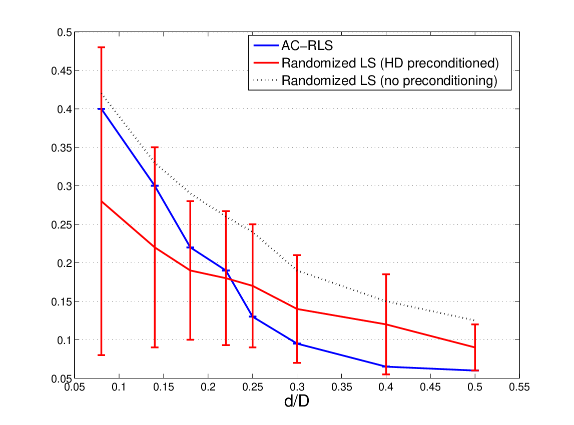
To further assess efficacy of the AC-RLS algorithm, real data tests were performed. The Protein Tertiary Structure dataset from the UCI Machine Learning Repository was tested. In this linear regression dataset, attributes of proteins are used to predict a value related to protein structure. A total of observations are included. Since the true is unknown, it is estimated by solving LS on the entire dataset. Subsequently, the noise variance is also estimated via sample averaging as . Figure 6 depicts relative squared-error (RSE) with respect to the data reduction ratio . The RSE curve for the HD-preconditioned LS corresponds to the average RSE across 50 runs, while the size of the vertical bars is proportional to its standard deviation. Different from RP-based methods, the RSE for AC-RLS does not entail standard deviation bars, because for a given initialization and data order, the output of the algorithm is deterministic. It can be observed that for the AC-RLS outperforms RPs in terms of estimating , while for very small , RPs yield a lower average RSE, at the cost however of very high error uncertainty (variance).
V-D Robust AC-RLS
To test rAC-LMS and rAC-RLS of Section IV-D, datasets were generated with , and , where ; noise was i.i.d. Gaussian ; meanwhile measurements were generated according to (1) with random and sporadic outlier spikes . Specifically, we generated , where , and , thus resulting in approximately of the data effectively being outliers. Similar to previous experiments, our novel algorithms were run once through the set selecting out of data to update . Plotted in Fig. 7 is the RSE averaged across 100 runs as a function of for the HD-preconditioned LS, the plain AC-RLS, and the rAC-RLS with a Huber-like instantaneous cost. As expected, the performance of AC-RLS is severely undermined especially when tuned for very small , exhibiting higher error than the RP-based LS. However, our rAC-RLS algorithm offers superior performance across the entire range of values.

VI Concluding Remarks
We developed online algorithms for large-scale LS linear regressions that rely on censoring for data-driven dimensionality reduction of streaming Big Data. First, a non-adaptive censoring setting was considered for applications where observations are censored – possibly naturally – separately and prior to estimation. Computationally efficient first- and second-order online algorithms were derived to estimate the unknown parameters, relying on stochastic approximation of the log-likelihood of the censored data. Performance was bounded analytically, while simulations demonstrated that the second-order method performs close to the CRLB.
Furthermore, online data reduction occurring parallel to estimation was also explored. For this scenario, censoring is performed deliberately and adaptively based on estimates provided by first- and second-order algorithms. Robust versions were also developed for estimation in the presence of outliers. Studied under the scope of stochastic approximation, the proposed algorithms were shown to enjoy guaranteed MSE performance. Moreover, the resulting recursive methods were advocated as low-complexity recursive solvers of large LS problems. Experiments run on synthetic and real datasets corroborated that the novel AC-LMS and AC-RLS algorithms outperformed competing randomized algorithms.
Our future research agenda includes approaches to nonlinear (e.g., kernel-based) parametric and nonparametric large-scale regressions, along with estimation of dynamical (e.g., state-space) processes using adaptively censored measurements.
Proof:
It can be verified that , which implies the convexity of [18]. The regret of the SGD approach is then bounded as [10, Corollary 2.7]
where is any sequence of estimates produced by the SA-MLE. By choosing , the aforementioned bound leads to Proposition 1. ∎
Proof:
For the SGD update in (23), the MSE , with where is bounded as in [30]. For this to hold, we must have: a1) the gradient bounded at the optimum; that is, ; a2) the gradient must be smooth for any other ; and a3) must be -strongly convex [30]. With and generated randomly and independently across time, associated quantities do not depend on . Furthermore, the points of discontinuity of are zero-measure in expectation, and thus are neglected for brevity.
Under a3), there exists a constant such that . Interchanging differentiation with expectation yields
It can be verified that the function is minimized for when . To see this, observe that its derivative vanishes when . Therefore, for all ; and hence,
for all and . The latter implies
showing that is strongly convex with . As expected, reduces for increasing .
Regarding the instantaneous gradient, it suffices to find such that for all and any pair . For the errors for , it holds
| (35) |
It can be verified that since the cross-terms in (35) can be bounded from below and above as
they are also equal to zero if the third-order moment . Furthermore, by simply bounding as probabilities, (35) yields
The last expression reveals that the average distance between gradients can be decomposed into two terms. The first term can be bounded using the fourth-order moment. The second term appears due to data censoring and clearly depends on , while it is assumed bounded as
Although we could not express in closed form, for relatively small values of used in practice to censor more than of the measurements, ; thus, the second term can be ignored yielding . Furthermore, even for large some inaccuracy in the value of can be tolerated, after considering that it does not affect the algorithm’s stability or asymptotic performance when a vanishing step size is used.
Finally, the expected norm of the gradient at is bounded and equal to
which completes the proof. ∎
Proof:
For the error vector , AC-RLS satisfies . If are deterministic and given, the error covariance matrix becomes
Assuming to be ergodic and for large enough , the matrix can be approximated by . Given that , we obtain
Since converges monotonically to , there exists such that for all
The result follows given that . ∎
References
- [1] K. Slavakis, G. B. Giannakis, and G. Mateos, “Modeling and optimization for big data analytics: Learning tools for our era of data deluge,” IEEE Sig. Proc. Mag., vol. 31, no. 5, pp. 18–31, Sept. 2014.
- [2] D. Donoho, “Compressed sensing,” IEEE Trans. Info. Theory, vol. 52, no. 4, pp. 1289–1306, Apr. 2006.
- [3] F. Pukelsheim, Optimal Design of Experiments. SIAM, 1993, vol. 50.
- [4] P. Drineas, M. W. Mahoney, and S. Muthukrishnan, “Sampling algorithms for regression and applications,” in Proc. of the 17-th Annual SIAM-ACM Symp. on Discrete Algorithms, 2006, pp. 1127–1136.
- [5] C. Boutsidis and P. Drineas, “Random projections for the nonnegative least-squares problem,” Linear Algebra and its Applications, vol. 431, no. 5, pp. 760–771, 2009.
- [6] M. Mahoney, “Randomized algorithms for matrices and data,” Found. Trends. in Mach. Learn., vol. 3, no. 2, pp. 123–224, 2011.
- [7] T. Strohmer and R. Vershynin, “A randomized Kaczmarz algorithm with exponential convergence,” J. of Fourier Analysis and Applications, vol. 15, no. 2, pp. 262–278, 2009.
- [8] D. Needell, N. Srebro, and R. Ward, “Stochastic gradient descent and the randomized Kaczmarz algorithm,” ArXiv e-prints. [Online]. Available: arXiv:1310.5715v2., 2014.
- [9] A. Agaskar, C. Wang, and Y. M. Lu, “Randomized Kaczmarz algorithms: Exact MSE analysis and optimal sampling probabilities,” in Proc. of Global Conf. on Signal and Info. Proc., Atlanta, Dec. 2014, pp. 389–393.
- [10] S. Shalev-Shwartz, “Online learning and online convex optimization,” Foundations and Trends in Machine Learning, pp. 107–194, 2011.
- [11] A. Ribeiro and G. B. Giannakis, “Bandwidth–constrained distributed estimation for wireless sensor networks–Part I: Gaussian case,” IEEE Trans. Sig. Proc., vol. 54, no. 3, pp. 1131–1143, Mar. 2006.
- [12] Y. Plan and R. Vershynin, “One-bit compressed sensing by linear programming,” IEEE Trans. Sig. Proc., vol. 66, no. 8, pp. 1275–1297, Aug. 2013.
- [13] G. Mateos, J. A. Bazerque, and G. B. Giannakis, “Distributed sparse linear regression,” IEEE Trans. Sig. Proc., vol. 58, no. 10, pp. 5262–5276, Oct. 2010.
- [14] T. Amemiya, “Tobit models: A survey,” J. Econom., vol. 24, no. 1, pp. 3–61, 1984.
- [15] L. Evers and C. M. Messow, “Sparse kernel methods for high-dimensional survival data,” Bioinformatics, vol. 14, no. 2, pp. 1632–1638, July 2008.
- [16] J. Tobin, “Estimation of relationships for limited dependent variables,” Econometrica: J. Econometric Soc., vol. 26, no. 1, pp. 24–36, 1958.
- [17] S. Maleki and G. Leus, “Censored truncated sequential spectrum sensing for cognitive radio networks,” IEEE J. Sel. Areas Commun., vol. 31, no. 3, pp. 364–378, 2013.
- [18] E. Msechu and G. B. Giannakis, “Sensor–centric data reduction for estimation with WSNs via censoring and quantization,” IEEE Trans. Sig. Proc., vol. 60, no. 1, pp. 400–414, 2012.
- [19] K. You, L. Xie, and S. Song, “Asymptotically optimal parameter estimation with scheduled measurements,” IEEE Trans. Sig. Proc., vol. 61, no. 14, pp. 3521–3531, July 2013.
- [20] G. Wang, J. Chen, J. Sun, and Y. Cai, “Power scheduling of Kalman filtering in wireless sensor networks with data packet drops,” arXiv preprint arXiv:1312.3269v2, 2013.
- [21] T. Y. Young and T. W. Calvert, Classification, Estimation and Pattern Recognition. North-Holland, 1974.
- [22] D. Bertsekas, Convex Optimization Algorithms. Athena Scientific, United States, 2015.
- [23] K. Slavakis, S.-J. Kim, G. Mateos, and G. Giannakis, “Stochastic approximation vis-a-vis online learning for big data analytics [lecture notes],” IEEE Sig. Proc. Mag., vol. 31, no. 6, pp. 124–129, 2014.
- [24] S. M. Kay, Fundamentals of Statistical Signal Processing, Vol. I: Estimation Theory. Englewood Cliffs: Prentice Hall PTR, 1993.
- [25] M. Mahoney, “Algorithmic and statistical perspectives on large-scale data analysis,” Combinatorial Scientific Computing, pp. 427–469, 2012.
- [26] D. P. Bertsekas and I. B. Rhodes, “Recursive state estimation for a set-membership description of uncertainty,” IEEE Trans. Autom. Control, vol. 16, no. 2, pp. 117–128, 1971.
- [27] S. Gollamudi, S. Nagaraj, S. Kapoor, and Y.-F. Huang, “Set-membership filtering and a set-membership normalized LMS algorithm with an adaptive step size,” IEEE Signal Processing Letters, vol. 5, no. 5, pp. 111–114, 1998.
- [28] Y. Hastie, R. Tibshirani, and J. Friedman, The Elements of Statistical Learning. Springer, 2009.
- [29] P. J. Huber, “Robust estimation of a location parameter,” The Annals of Mathematical Statistics, vol. 35, no. 1, pp. 73–101, 1964.
- [30] E. Moulines and F. R. Bach, “Non-asymptotic analysis of stochastic approximation algorithms for machine learning,” in Proc. of Advances in Neural Info. Proc. Sys. Conf., Granada, Spain, 2011, pp. 451–459.