Estimating an Activity Driven Hidden Markov Model

David A. Meyer and Asif Shakeel Address: Department of Mathematics, University of California/San Diego, La Jolla, CA 92093-0112, USA Email address: dmeyer@math.ucsd.edu, ashakeel@ucsd.edu

Date: August 24, 2026

Abstract.

We define a Hidden Markov Model (HMM) in which each hidden state has time-dependent activity levels that drive transitions and emissions, and show how to estimate its parameters. Our construction is motivated by the problem of inferring human mobility on sub-daily time scales from, for example, mobile phone records.

1. Introduction

Hidden Markov models (HMMs) are stochastic models for systems with a set of unobserved states between which the system hops stochastically, sometimes emitting a signal from some alphabet, with probabilities that depend upon the current state. The situation in which we are specifically interested is human mobility, partially observed, i.e., occasional signals about a person’s location. For example, consider the cells of a mobile phone network, from which a user can make calls. In this case the states of a HMM are the cells, and the emitted signals are the cell itself, if a call is made by a particular user during each of a sequence of time intervals, or nothing (0), if that user does not make a call. In the latter case, the state (location) of the user is ‘hidden’, and must be inferred, while in the former case, assuming no errors in the data, the ‘hidden’ state is revealed by the call record.¹¹ 1 Load balancing, in which calls may be routed through cell towers that are not the closest, makes this not strictly true. The general model we consider here allows for this possibility. Since these are data from a mobile phone network, a user can move from cell to cell.

Although many analyses of human mobility have estimated no more than rather crude statistics like the radius of gyration, the fraction of time spent at each location, or the entropy of the timeseries of locations [9, 16, 3, 12], others have used HMMs to describe partially observed human mobility and have estimated their parameters [8, 13, 14]. With short time steps, however, a standard HMM (with time-independent parameters) is not a plausible model, since human mobility behavior changes according to, for example, the time of day [10, 16, 3, 2]. We would like to create, therefore, a HMM with time-dependent parameters. Of course, allowing, for example, arbitrary transition/emission probabilities at each time step, would lead to an extremely underdetermined model. Rather, we need a model with only a few additional parameters to capture the time-dependence of human mobility. Since the total numbers of trips [10, 16, 2] and mobile phone calls [3, 6] vary with time of day and day of week, we develop a time-dependent HMM in which the non-trivial transition and emission probabilities are proportional to activity levels, i.e., to some given functions modeling how active humans are at different times and places.

Since the transition and emission probabilities in our HMM are not constant in time, it is a non-stationary HMM. Many generalizations of HMMs have been considered previously, of course, as more faithful models of various real systems. Some of these are non-stationary: Deng, for example, considers a class of models in which the emission probabilities are somewhat non-Markovian, depending on a number of previous emissions, and also have polynomial-in-time trend components which are to be estimated [5]. Duration HMMs (DHMMs), first suggested by Ferguson [7], allow a sort of non-stationarity in the state transition process by including a randomly chosen duration each time the state changes, i.e., a number of time steps without a transition away from that state. This kind of model has been generalized to make the transition probabilities functions of the number of steps the system has been in the current state [15]. In a different direction, since one can think of transitions between the hidden states with different emission probability distributions as a kind of non-stationarity, triplet Markov chains (TMCs) include an auxiliary set of underlying states, each of which corresponds to a different stationary regime for a HMM [11]. Our approach is different than that of DHMMs and TMCs in that the time dependence of the transition and emission probabilities is not intrinsic and random, but rather exogenous and deterministic. Furthermore, unlike Deng’s models [5], we take the “trend” part of the time dependence to be given, not an additional (set of) parameter(s) to be estimated.

Formally, our model consists of $N$ possible hidden states, and we denote by $(X_{t})\in[N]^{T}$ the time series of $T$ hidden states (for any $n\in\mathbb{N}$ , $[n]=\{1,\ldots,n\}$ ). State transitions happen according to a sequence of matrices giving the conditional probabilities of transitions,

A(t)=\bigl(a_{ij}(t)\bigr),{\rm\ where\ }a_{ij}(t)=\Pr(X_{t+1}=i\mid X_{t}=j).

At each state we observe an emission that takes a value from the set $[M]\cup\{0\}$ , where $0$ denotes “absence of an emission”. Let $y=(y_{t})\in([M]\cup\{0\})^{T}$ be the series of observed emissions. The probability of emission $s$ at time $t$ , from state $j$ , is

b_{sj}(t)=\text{Pr}(Y_{t}=s\mid X_{t}=j).

We define time varying activity levels for state $j$ by a pair of functions with non-negative values, $(f_{j},g_{j}):[T]\to[0,1]^{2}$ , the activity functions, which modulate transitions and emissions from the state, respectively. Given a state $j$ , the transition probabilities from that state are functions of transition parameters $(\tau_{ij}\geq 0)$ , $i\neq j\in[N]$ , and the activity level:

(1)

a_{ij}(t)=\left\{\begin{array}[]{ll}f_{j}(t)\tau_{ij}&\text{if }i\neq j;\\ 1-f_{j}(t)\sum_{i\in[N],i\neq j}\tau_{ij}&\text{if }i=j,\end{array}\right.

subject to the constraints that for all $j\in[N]$ and all $t\in[T]$ ,

(2)

f_{j}(t)\sum_{i\in[N],i\neq j}\tau_{ij}\leq 1.

In practice we may have a priori knowledge that some transitions do not occur, so that $(a_{ij})$ (and $(\tau_{ij})$ ) have some entries set to $0$ . For example, with 10 minute time intervals and states representing cells in a mobile phone network, transitions between sufficiently distant cells are precluded.

Similarly, we assign emission parameters $(\epsilon_{sj}\geq 0)$ , $s\in[M]$ , to each state $j$ . The emission probabilities are

(3)

b_{sj}(t)=\left\{\begin{array}[]{ll}g_{j}(t)\epsilon_{sj}&\text{if }s\neq 0;\\ 1-g_{j}(t)\sum_{s\in[M]}\epsilon_{sj}&\text{if }s=0,\end{array}\right.

subject to the constraints that for all $j\in[N]$ and all $t\in[T]$ ,

(4)

g_{j}(t)\sum_{s\in[M]}\epsilon_{sj}\leq 1.

Denote the initial distribution over states by $\pi_{j}=\Pr(X_{1}=j)$ , subject to the constraints $\pi_{j}\geq 0$ and

(5)

\sum_{j\in[N]}\pi_{j}=1.

Were this a typical hidden Markov model, we could estimate its parameters using the Baum-Welch algorithm [1, 17]. Since it is not, we develop a novel Expectation Maximization (EM) algorithm [4] to estimate the parameters $\Theta=\big((\pi_{j}),(\tau_{ij}),(\epsilon_{sj})\big)$ , given $y$ , $f_{j}(t)$ and $g_{j}(t)$ , as follows.

2. Expectation Maximization

The expectation maximization algorithm maximizes, at each iterative step, the (expected) log-likelihood function described below. Let $\mathcal{X}$ be the set of all possible time series of states and let ${\hat{\Theta}}^{k}$ be the estimate of $\Theta$ at the $k$ -th iteration of the algorithm.

(6)

{\hat{\Theta}}^{k}=\big((\hat{\pi}^{k}_{j}),(\hat{\tau}^{k}_{ij}),(\hat{\epsilon}^{k}_{sj})\big).

The algorithm begins by initializing the parameter estimates in the first ( $k=1$ ) iteration. Then the $k+1^{\rm st}$ iteration consists of two steps:

(i)

Compute the expectation value of the log-likelihood, using the current ( $k^{\rm th}$ ) estimate for the parameters:

(7) $\mathcal{L}(\Theta,{\hat{\Theta}}^{k})=\sum_{x\in\mathcal{X}}\log[\Pr(x,y;\Theta)]\Pr(x\mid y;{\hat{\Theta}}^{k}),$

where $\Pr(\cdot;\Theta)$ means $\Pr(\cdot)$ in a probability distribution parametrized by $\Theta$ .
(ii)

Find the parameters that maximize the expected log-likelihood:

${\hat{\Theta}}^{k+1}=\underset{\Theta}{\argmax}\>\mathcal{L}(\Theta,{\hat{\Theta}}^{k}),$

subject to constraints in the inequalities (2), (4) and (5).

As in the regular Baum-Welch algorithm, we express our computations in terms of certain conditional probabilities based on the parameters estimated at the $k^{\rm th}$ iteration,

(8)		$\displaystyle\gamma^{k}_{j}(t)$	$\displaystyle=\Pr(X_{t}=j\mid y;{\hat{\Theta}}^{k}),$
(8)		$\displaystyle\xi^{k}_{ij}(t)$	$\displaystyle=\Pr(X_{t}=j,X_{t+1}=i\mid y;{\hat{\Theta}}^{k}).$

Some reindexing of eq. (7) yields the following expression for $\mathcal{L}(\Theta,{\hat{\Theta}}^{k})$ in terms of these probabilities:

(9)

\mathcal{L}(\Theta,{\hat{\Theta}}^{k})=\sum_{j\in[N]}\log(\pi_{j})\gamma^{k}_{j}(1)+\sum_{i,j\in[N]}\sum_{t=1}^{T-1}\log\bigl(a_{ij}(t)\bigr)\xi^{k}_{ij}(t)+\sum_{j\in[N]}\sum_{t=1}^{T}\log\bigl(b_{y_{t}j}(t)\bigr)\gamma^{k}_{j}(t).

We iterate steps (i) and (ii), for which we compute $\gamma^{k}_{j}(t)$ and $\xi^{k}_{ij}(t)$ in eqs. (8), and $\mathcal{L}(\Theta,{\hat{\Theta}}^{k})$ in eq. (9) above. We continue until some standard of convergence is achieved. We then output the final ${\hat{\Theta}}^{k}$ as our estimate of $\Theta$ .

Theorem 2.1.

There is a constrained expectation maximization algorithm giving a sequence of estimates $\hat{\Theta}^{k}$ that converges to a critical point of the likelihood function, which is the maximum likelihood estimate $\hat{\Theta}$ for the observed sequence $y$ when the initial guess is sufficiently close. Further, to achieve a precision $\epsilon$ in the estimates, the time complexity of the algorithm is $O\bigl((N^{2}+M)T\log(T/\epsilon)\bigr)$ . In particular, for a fixed precision $\epsilon$ , the time complexity is $O\bigl((N^{2}+M)T\log T\bigr)$ .

Proof.

Suppose we have the estimates $\hat{\Theta}^{k}$ defined in eq. (6) from step $k$ of the algorithm. We proceed to compute $\gamma^{k+1}_{j}(t)$ and $\xi^{k+1}_{ij}(t)$ in eqs. (8) to begin the next iteration. Just as in the regular Baum-Welch algorithm, we apply dynamic programming. Denote the $k^{\rm th}$ estimate of the transition matrix by $\hat{A}^{k}(t)=\bigl(\hat{a}^{k}_{ij}(t)\bigr)$ , where

(10)

\hat{a}^{k}_{ij}(t)=\left\{\begin{array}[]{ll}f_{j}(t)\hat{\tau}^{k}_{ij}&\text{if }i\neq j;\\ 1-f_{j}(t)\sum_{i\neq j}\hat{\tau}^{k}_{ij}&\text{if }i=j.\end{array}\right.

Similarly,

(11)

\hat{b}^{k}_{sj}(t)=\left\{\begin{array}[]{ll}g_{j}(t)\hat{\epsilon}^{k}_{sj}&\text{if }s\neq 0;\\ 1-g_{j}(t)\sum_{s\in[M]}\hat{\epsilon}^{k}_{sj}&\text{if }s=0.\end{array}\right.

It is convenient to define $\hat{B}^{k}(t)$ to be the diagonal matrix with $jj^{\rm th}$ entry $\hat{b}^{k}_{y_{t}j}(t)$ . Now compute two sequences of (co)vectors, $\alpha^{k}(t)\in\mathbb{R}^{N}$ and $\beta^{k}(t)\in(\mathbb{R}^{N})^{\dagger}$ , recursively, as follows:

	$\displaystyle\alpha^{k}(1)$	$\displaystyle=\hat{B}^{k}(1)\hat{\pi}^{k};$
	$\displaystyle\alpha^{k}(t)$	$\displaystyle=\hat{B}^{k}(t)\hat{A}^{k}(t-1)\alpha^{k}(t-1);$
	$\displaystyle\beta^{k}(T)$	$\displaystyle={\bf 1}^{\mathsf{T}}\hat{B}^{k}(T);$
	$\displaystyle\beta^{k}(t)$	$\displaystyle=\beta^{k}(t+1)\hat{A}^{k}(t)\hat{B}^{k}(t).$

Then²² 2 With a slight notational abuse, $\hat{B}^{k}(t)^{-1}$ denotes the diagonal matrix whose $jj^{\rm th}$ entry is $1/\hat{b}^{k}_{y_{t}j}(t)$ if $\hat{b}^{k}_{y_{t}j}(t)\neq 0$ and $1$ otherwise.

	$\displaystyle\gamma^{k+1}_{j}(t)$	$\displaystyle={\beta^{k}_{j}(t)\hat{b}^{k}_{y_{t}j}(t)^{-1}\alpha^{k}_{j}(t)\over\beta^{k}(t)\hat{B}^{k}(t)^{-1}\alpha^{k}(t)};$
	$\displaystyle\xi^{k+1}_{ij}(t)$	$\displaystyle={\beta^{k}_{i}(t+1)\hat{a}^{k}_{ij}(t)\alpha^{k}_{j}(t)\over\beta^{k}(t+1)\hat{A}^{k}(t)\alpha^{k}(t)}.$

The estimates for the initial probabilities $\pi_{j}$ are the same as in the normal Baum-Welch algorithm, as is clear from the expression for $\mathcal{L}(\Theta,{\hat{\Theta}}^{k})$ in eq. (9). Thus

\hat{\pi}^{k+1}_{j}=\gamma^{k+1}_{j}(1).

Now notice that all the constraints in (2) and (4) necessary to define $\mathcal{L}(\Theta,{\hat{\Theta}}^{k})$ are implied by the strongest constraints: for all $j\in[N]$ ,

(12)

f^{*}_{j}\sum_{r\neq j}\tau_{rj}\leq 1,

where $f^{*}_{j}=\max_{t\in[T-1]}\>f_{j}(t)$ , and

(13)

g^{*}_{j}\sum_{s\in[M]}\epsilon_{sj}\leq 1,

where $g^{*}_{j}=\max_{t\in[T]}\>g_{j}(t)$ .

Consider the computation of $\hat{\tau}^{k+1}_{ij}$ , for $i\neq j\in[N]$ . It should lie in the domain $F_{j}\subset\mathbb{R}^{N}$ defined by constraints (12) and the non-negativity of the parameters. Since these constraints are independent for different $j$ s, we can consider each $j$ separately, and find the optimal parameters $\tau_{ij}$ by computing the critical points of $\mathcal{L}(\Theta,{\hat{\Theta}}^{k})$ relative to $(\tau_{ij})\in F_{j}$ . Using eqs. (9) and (1),

(14)

\frac{\partial\mathcal{L}(\Theta,{\hat{\Theta}}^{k})}{\partial\tau_{ij}}=\frac{1}{\tau_{ij}}\sum_{t=1}^{T-1}\xi^{k}_{ij}(t)-\sum_{t=1}^{T-1}\frac{f_{j}(t)\xi^{k}_{jj}(t)}{1-f_{j}(t)\sum_{r\neq j}\tau_{rj}}

If the left sum in eq. (14), $\sum_{t=1}^{T-1}\xi^{k}_{ij}(t)=0$ , the derivative is nonpositive, so $\mathcal{L}(\Theta,{\hat{\Theta}}^{k})$ is weakly decreasing and $\tau_{ij}=0$ gives its largest value. If the right sum in eq. (14), $\sum_{t=1}^{T-1}f_{j}(t)\xi^{k}_{jj}(t)/(1-f_{j}(t)\sum_{r\neq j}\tau_{rj})=0$ , the derivative is nonnegative, so $\mathcal{L}(\Theta,{\hat{\Theta}}^{k})$ is weakly increasing and takes its maximum value when $\tau_{ij}$ is as large as possible, i.e., when it saturates constraint (12). We will show how to handle this situation after discussing the generic case which we do next.

Assuming then that neither sum in eq. (14) is $0$ , to find the stationary points of $\mathcal{L}(\Theta,{\hat{\Theta}}^{k})$ we set eq. (14) to $0$ and solve for $\tau_{ij}$ . Specifically, $\tau_{ij}$ must satisfy

(15)

\frac{1}{\tau_{ij}}\sum_{t=1}^{T-1}\xi^{k}_{ij}(t)=\sum_{t=1}^{T-1}\frac{f_{j}(t)\xi^{k}_{jj}(t)}{1-f_{j}(t)\sum_{r\neq j}\tau_{rj}}.

We note that if $f_{j}(t)\equiv 1$ , which makes the transition probabilities, $a_{ij}$ , time independent, then the solution to eq. (15) is the familiar Baum-Welch solution: $\hat{a}^{k}_{ij}=\hat{\tau}^{k}_{ij}=\sum_{t=1}^{T-1}\xi^{k}_{ij}(t)/\sum_{t=1}^{T-1}\gamma_{j}(t)$ for all $i,j\in[N]$ . For non-constant activity functions, however, the solution is more complicated.

Since the right side of eq. (15) is manifestly independent of $i$ , the left side must be, too. Let

(16)

\tau_{j}=\frac{\tau_{ij}}{\sum_{t=1}^{T-1}\xi^{k}_{ij}(t)}=\frac{\tau_{ij}}{\Xi^{k}_{ij}},

where the last expression uses the antiderivative convention that for a function of $t$ denoted by a letter in lower case, the corresponding upper case letter³³ 3 $\Xi$ is upper case $\xi$ ; $\Lambda$ is upper case $\lambda$ ; $M$ is upper case $\mu$ ; $N$ is upper case $\nu$ ; $\Gamma$ is upper case $\gamma$ . represents its sum over its domain of definition ( $t=1$ to $T-1$ in this case). Now

\sum_{r\neq j}\tau_{rj}=\tau_{j}\sum_{r\neq j}\Xi^{k}_{rj}=\tau_{j}\sum_{t=1}^{T-1}\sum_{r\neq j}\xi^{k}_{rj}(t).

If we denote the probability of moving away from state $j$ by

\mu^{k}_{j}(t)=\sum_{r\neq j}\xi^{k}_{rj}(t),

we can write $\sum_{r\neq j}\tau_{rj}=\tau_{j}M^{k}_{j}$ . Substituting in eq. (15), this gives:

\frac{1}{\tau_{j}}=\sum_{t=1}^{T-1}\frac{f_{j}(t)\xi^{k}_{jj}(t)}{1-f_{j}(t)M^{k}_{j}\tau_{j}},

or equivalently:

(17)

1=\sum_{t=1}^{T-1}\frac{f_{j}(t)\xi^{k}_{jj}(t)}{1/\tau_{j}-f_{j}(t)M^{k}_{j}}.

We must solve this equation for $\tau_{j}$ , whence we can use eq. (16) to solve for each of the $\tau_{ij}$ . Since $\tau_{j}$ is nonnegative and constraint (12) must hold, we recast these conditions in terms of $\tau_{j}$ as:

f^{*}_{j}M^{k}_{j}<\frac{M_{j}^{k}}{\sum_{r\neq j}\tau_{rj}}=\frac{1}{\tau_{j}}<\infty.

Let

f^{k*}_{j}=\max_{t\in[T-1]\,\mid\,\xi^{k}_{jj}(t)\neq 0}\>f_{j}(t)\,\,\leq f^{*}_{j}.

Each of the terms in the sum on the right side of eq. (17) is strictly decreasing in $1/\tau_{j}$ when it is well-defined ( $1/\tau_{j}>f^{k*}_{j}M^{k}_{j}$ ). Values of $1/\tau_{j}$ just larger than $f^{k*}_{j}M^{k}_{j}$ make the sum arbitrarily large, and as $1/\tau_{j}$ increases from that value, the sum decreases monotonically to 0, so exactly one value of $\tau_{j}<1/(f^{k*}_{j}M^{k}_{j})$ will satisfy eq. (17). We can solve the equation numerically to find this value, call it $\tau^{c}_{j}$ . If $\tau^{c}_{j}<1/(f^{*}_{j}M^{k}_{j})$ , splitting it proportionally to $\Xi_{ij}$ according to eq. (16) gives the unique critical point $(\tau_{ij})\in F_{j}$ of $\mathcal{L}(\Theta,{\hat{\Theta}}^{k})$ .

We can compute explicitly the Hessian of $\mathcal{L}(\Theta,{\hat{\Theta}}^{k})$ with respect to the $\tau_{ij}$ ; its components are:

\frac{\partial^{2}\mathcal{L}(\Theta,{\hat{\Theta}}^{k})}{\partial\tau_{ij}\partial\tau_{i^{\prime}j}}=-\frac{\Xi^{k}_{ij}}{\tau^{2}_{ij}}\delta_{ii^{\prime}}-\sum_{t=1}^{T-1}\frac{f^{2}_{j}(t)\xi^{k}_{jj}(t)}{(1-f_{j}(t)\sum_{r\neq j}\tau_{rj})^{2}}.

Thus, as a matrix the Hessian can be written as the sum of two matrices:

\left(\frac{\partial^{2}\mathcal{L}(\Theta,{\hat{\Theta}}^{k})}{\partial\tau_{ij}\partial\tau_{i^{\prime}j}}\right)=-\begin{pmatrix}\Xi^{k}_{1j}/\tau^{2}_{1j}\\ &\ddots\\ &&\Xi^{k}_{Nj}/\tau^{2}_{Nj}\end{pmatrix}-\sum_{t=1}^{T-1}\frac{f^{2}_{j}(t)\xi^{k}_{jj}(t)}{(1-f_{j}(t)\sum_{r\neq j}\tau_{rj})^{2}}\,{\bf 1}{\bf 1}^{\mathsf{T}},

where ${\bf 1}\in\mathbb{R}^{N}$ is the vector of all $1$ s. Each of the matrices on the right is negative semi-definite, so the Hessian is also. Thus the (unique) critical point we found in this case is a global maximum of $\mathcal{L}(\Theta,{\hat{\Theta}}^{k})$ in $F_{j}$ and hence the choice for $\hat{\tau}_{ij}^{k+1}$ .

If the solution does not satisfy the original constraint (12), i.e., $\tau^{c}_{j}\geq 1/(f^{*}_{j}M^{k}_{j})$ , or if the right side of eq. (15) is $0$ , the maximum will be on the boundary of $F_{j}$ . Thus we maximize $\mathcal{L}(\Theta,{\hat{\Theta}}^{k})$ subject to the boundary constraint

\sum_{j\neq i\in[N]}\tau_{ij}=\frac{1}{f^{*}_{j}}.

This is in the form of the constraint in the regular Baum-Welch algorithm with 1 replaced by $1/f^{*}_{j}$ and the self-transition probability set to 0. Thus the critical $\tau_{ij}$ can be computed as in the Baum-Welch algorithm,⁴⁴ 4 In our notation, the usual Baum-Welch estimate is $\hat{a}^{k}_{ij}=\hat{\tau}^{k}_{ij}=\Xi^{k}_{ij}/\Gamma^{k}_{j}$ for all $i,j$ . with $\Gamma^{k}_{j}$ replaced by $M^{k}_{j}$ and the solution divided by $f^{*}_{j}$ :

\tau^{c}_{ij}=\frac{\Xi^{k}_{ij}}{f^{*}_{j}M^{k}_{j}}.

This is the unique critical point in this case, and the global maximum of $\mathcal{L}(\Theta,{\hat{\Theta}}^{k})$ in $F_{j}$ , by the same argument as in the Baum-Welch algorithm. This becomes the choice for $\hat{\tau}_{ij}^{k+1}$ .

We turn to the computation of $\hat{\epsilon}_{sj}^{k+1}$ , $s\in[M]$ . As before, we begin by finding the stationary points of $\mathcal{L}(\Theta,{\hat{\Theta}}^{k})$ , now relative to $(\epsilon_{sj})\in G_{j}\subset\mathbb{R}^{M}$ defined by constraints (13) and the non-negativity of these parameters. Using eqs. (9) and (3) gives:

(18)

\frac{\partial\mathcal{L}(\Theta,{\hat{\Theta}}^{k})}{\partial\epsilon_{sj}}=\frac{1}{\epsilon_{sj}}\sum_{t=1}^{T}\gamma^{k}_{j}(t)\delta_{s,y_{t}}-\sum_{t=1}^{T}\frac{g_{j}(t)\gamma^{k}_{j}(t)}{1-g_{j}(t)\sum_{l\in[M]}\epsilon_{lj}}\delta_{0,y_{t}}.

As we did for eq. (14), we must consider the situations when either of the sums in eq. (18) vanishes. When the left sum is $0$ , a extreme value is given by $\epsilon_{sj}=0$ , and when the right sum is $0$ , constraint (13) is saturated. Assuming neither of the sums vanishes, we find the stationary points by solving

(19)

\frac{1}{\epsilon_{sj}}\sum_{t=1}^{T}\gamma^{k}_{j}(t)\delta_{s,y_{t}}=\sum_{t=1}^{T}\frac{g_{j}(t)\gamma^{k}_{j}(t)}{1-g_{j}(t)\sum_{l\in[M]}\epsilon_{lj}}\delta_{0,y_{t}}.

Solution to the emission equations, eqs. (19), follows using the same steps as for the transition equations, eqs. (15). We first denote the probability of emission $s\in[M]$ from state $j$ by:⁵⁵ 5 In a simplified model for the mobile phone data we discussed in the Introduction, $M=N$ and every state $j$ emits either the signal $j$ or $0$ ; in other words, $\epsilon_{sj}=0$ if $s\neq j\in[M]$ . This simplifies the following expressions: For $t$ such that $y_{t}=j$ , $\gamma^{k}_{j}(t)=1$ (the state is $j$ with certainty if the observed emission is $j$ ), i.e., $\lambda^{k}_{jj}(t)=\delta_{j,y_{t}}$ , and $\lambda^{k}_{sj}(t)=0$ if $s\neq j\in[M]$ .

\lambda^{k}_{sj}(t)=\gamma^{k}_{j}(t)\delta_{s,y_{t}},

in terms of which we rewrite eq. (19) as

(20)

\frac{1}{\epsilon_{sj}}\sum_{t=1}^{T}\lambda^{k}_{sj}(t)=\sum_{t=1}^{T}\frac{g_{j}(t)\lambda^{k}_{0j}(t)}{1-g_{j}(t)\sum_{l\in[M]}\epsilon_{lj}}.

We define (independent of $s$ )

(21)

\epsilon_{j}=\frac{\epsilon_{sj}}{\Lambda^{k}_{sj}}.

We also define the probability of any non-zero emission from state $j$ ,

\nu^{k}_{j}(t)=\sum_{l\in[M]}\lambda^{k}_{lj}(t),

which, used in eq. (20), gives

(22)

1=\sum_{t=1}^{T}\frac{g_{j}(t)\lambda^{k}_{0j}(t)}{1/\epsilon_{j}-g_{j}(t)N^{k}_{j}}.

Let

g^{k*}_{j}=\max_{t\in[T]\,\mid\,\lambda^{k}_{0j}(t)\neq 0}\>g_{j}(t)\,\,\leq g^{*}_{j}.

As before, there is exactly one solution $\epsilon^{c}_{j}<1/(g^{k*}_{j}N^{k}_{j})$ to eq. (22). We can find it numerically, and if $\epsilon^{c}_{j}<1/(g^{*}_{j}N^{k}_{j})$ , we use eq. (21) to find all the $\epsilon_{sj}$ , which will then satisfy constraint (13). Again we can compute the Hessian explicitly to confirm that this is a global maximum of $\mathcal{L}(\Theta,{\hat{\Theta}}^{k})$ , now in $G_{j}$ , and hence the choice for $\hat{\epsilon}_{sj}^{k+1}$ .

If $\epsilon^{c}_{j}\geq 1/(g^{*}_{j}N^{k}_{j})$ , or if the right side of eq. (20) is $0$ , we must find instead the critical point on the boundary of $G_{j}$ :

\sum_{s\in[M]}\epsilon_{sj}=\frac{1}{g^{*}_{j}}.

Again, this is in the form of the constraint in the regular Baum-Welch algorithm. Accordingly, we set the critical $\epsilon_{sj}$ to the Baum-Welch estimate, rescaled by $g^{*}_{j}$ :

\epsilon^{c}_{sj}=\frac{\Lambda^{k}_{sj}}{g^{*}_{j}N^{k}_{j}}.

This is the unique critical point and the global maximum of $\mathcal{L}(\Theta,{\hat{\Theta}}^{k})$ in $G_{j}$ , and therefore the choice for $\hat{\epsilon}_{sj}^{k+1}$ in this case.

We have shown how to find ${\hat{\Theta}}^{k+1}$ maximizing $\mathcal{L}(\Theta,{\hat{\Theta}}^{k})$ in eq. (9). This algorithm converges as claimed because it is an instance of expectation maximization. To understand its time complexity we must consider the numerical solution of eqs. (17) and (22). To simplify notation we rewrite eq. (17) in terms of $u=1/\tau_{j}$ , and a function $w(u)$ ,

(23)

w(u)=\sum_{t=1}^{T-1}\frac{f_{j}(t)\xi^{k}_{jj}(t)}{u-f_{j}(t)M^{k}_{j}}-1,

as $w(u)=0$ . As an initial estimate for the root, $u^{c}$ , we can use $u^{L}>f^{k*}_{j}M^{k}_{j}$ such that

(24)

\frac{f^{k*}_{j}\xi^{k}_{jj}(t^{k*}_{j})}{u^{L}-f^{k*}_{j}M^{k}_{j}}=1,

where $t^{k*}_{j}\in[T-1]$ satisfies $f_{j}(t^{k*}_{j})=f^{k*}_{j}$ and $\xi^{k}_{jj}(t^{k*}_{j})\neq 0$ . $u^{L}\leq u^{c}$ since we found it using only one of the nonnegative terms in the sum in eq. (23).

Now recall that $f_{j}(t)\xi^{k}_{jj}(t)\leq f^{k*}_{j}$ for $t\in[T-1]$ , and

0\leq M^{k}_{j}=\sum_{t\in[T-1]}\mu^{k}_{j}(t)=\sum_{t\in[T-1]}\sum_{r\neq j}\xi^{k}_{rj}(t)\leq\sum_{t\in[T-1]}\gamma^{k}_{j}(t)\leq T-1.

Thus each term in the sum in eq. (23) is no more than

\frac{f^{k*}_{j}}{u-(T-1)f^{k*}_{j}}.

At $u^{R}=2(T-1)f^{k*}_{j}$ this is $1/(T-1)$ , so $w(u^{R})\leq 0$ , which implies

(25)

u^{L}\leq u^{c}\leq u^{R}=2(T-1)f^{k*}_{j}.

Using Newton’s method, once we have an initial estimate “sufficiently close” to the root of $w(u)=0$ , the time complexity to find it with error less than $\epsilon$ is $O\bigl(T\log(1/\epsilon)\bigr)$ , where the $T$ comes from the cost of evaluating $w(u)$ and $w^{\prime}(u)$ at each iteration; in practice this is how we would find the root. Since the length of the interval in (25) is $O(T)$ , however, the bisection method gets us to precision $\epsilon$ with $O\bigl(\log(T/\epsilon)\bigr)$ steps, with total cost $O\bigl(T\log(T/\epsilon)\bigr)$ ; thus this is the total complexity.

We need to solve eqs. (17) and (22) $N$ and $M$ times, respectively, at each iteration, which thus adds $O\bigl((N+M)T\log(T/\epsilon)\bigr)$ to the $O(N^{2}T)$ complexity of the computations for $\gamma^{k+1}_{i}$ and $\xi^{k+1}_{ij}$ . Thus the time complexity for the whole algorithm is $O\bigl((N^{2}+M)T\log(T/\epsilon)\bigr)$ . ∎

3. Numerical Simulations

To demonstrate the effect of the activity functions we consider a simple model with $N=3$ states and the same number of possible emissions ( $M=3$ ). From any state $j$ , we only allow an emission to be either its own label $j$ or $0$ , i.e., $\epsilon_{sj}=0$ for $j\neq s\in[M]$ , so a non-zero emission uniquely identifies the state that emits it. We choose random transition and emission parameters:

	$\displaystyle(\epsilon_{jj})$	$\displaystyle=(0.770347,0.579213,0.0821789);$
	$\displaystyle(\tau_{ij})$	$\displaystyle=\left(\begin{array}[]{ccc}&0.298244&0.0621274\\ 0.134788&&0.3710750\\ 0.383490&0.182008&\\ \end{array}\right),$

where the omitted values are the components for which $i=j$ .

We generate sequences of length $T=24\cdot 6\cdot 7\cdot 200$ (we may think of this as $200$ weeks, with an observation every $10$ minutes). We consider activity functions with variations that may approximate observed data, i.e., periodic variations with a period of $24\cdot 6$ (one day). Specifically, our numerical simulations use the following three functions:

(i)

constant function,

$\mathit{1}(t)=1;$
(ii)

raised cosine,

$r_{n}(t)=\frac{n-\cos\left(2\pi t/(24\cdot 6)\right)}{n+1};$
(iii)

shifted cosine

$c_{j}(t)=\frac{1}{3}\left[2-\cos\left(\frac{2\pi(t-6j)}{24\cdot 6}\right)\right].$

We generate a random sequence of states, $x$ , and resulting emissions, $y$ , using the transition and emission parameters above, and a pair of activity functions (a list of these pairs is shown in Table 2).

Before computing the sequence of parameter estimates, we need to specify how we compute initial estimates to start the iteration. This can only depend on the observed emission sequence $y$ , since in any real scenario $x$ is unknown. As a first guess, for this simple model, we interpolate the state sequence $x$ as follows:⁶⁶ 6 For more general models, finding initial parameter estimates will be more complicated, depending on the particulars of the model. For every pair of successive non-zero emissions, there is a segment of zeros (no emission) separating them. We divide each such segment into two subsegments: Let $j\in[M]$ be the emission immediately preceding the segment, and $i\in[M]$ be the emission immediately following the segment. The second subsegment starts at the first time step after the one where $f_{j}$ first attains its maximum value on the segment (i.e., a time at which there is the maximum probability of hopping from state $j$ to state $i$ ). We assign state $j$ to the time steps in the first subsegment and the state $i$ to those in the second. If the emission sequence $y$ starts with a segment of zeros, then that segment is assigned the value of the first non-zero emission; similarly a terminal sequence of zeros is given the value of the last non-zero emission. Denote the interpolated states by $z=(z_{t})$ , $t\in[T]$ .

From $z$ , we compute the estimate $(\hat{\pi}^{1}_{j})$ for the initial distribution over the states $(\pi_{j})$ by their frequencies of occurrence. For the initial $\tau_{ij}$ estimate, $\hat{\tau}^{1}_{ij}$ , we use the method described in the proof of Theorem 2.1 to solve eq. (14), using $\xi^{k}_{ij}(t)=\delta_{i,z_{t+1}}\delta_{j,z_{t}}$ , including $i=j$ . For the initial $\epsilon_{jj}$ estimate, $\hat{\epsilon}^{1}_{jj}$ , we also use the method described in the proof of Theorem 2.1 to solve eq. (18), using $\gamma_{j}(t)=\delta_{j,z_{t}}$ .

To understand the performance of the algorithm in Theorem 2.1, we need a measure of the error between the estimates and the real parameter values. The relative entropy is one measure for a stationary HMM. In our case we need to account for the time variation of the transition and emission probabilities, $a_{ij}(t)$ and $b_{sj}(t)$ . Hence we define a modified version of a relative entropy error criterion, the averaged relative entropy.

Definition 3.1.

Let $\mathcal{Q}=(Q_{t})$ and $\mathcal{P}=(P_{t})$ , $t\in[T]$ , be two finite sequences of discrete probability distributions on a finite set $\mathcal{I}$ . The Averaged Relative Entropy ( $\mathsf{ARE}$ ) of $\mathcal{P}$ with respect to $\mathcal{Q}$ is

\mathsf{ARE}(\mathcal{P},\mathcal{Q})=\frac{1}{T}\sum_{t\in[T]}\mathsf{RE}(P_{t},Q_{t}),

where the usual relative entropy ( $\mathsf{RE}$ ) is given by

\mathsf{RE}(P_{t},Q_{t})=\sum_{i\in\mathcal{I}}P_{t}(i)\log\frac{P_{t}(i)}{Q_{t}(i)}.

Thus the error function that we compute for given $(\tau_{ij})$ and estimate $(\hat{\tau}^{k}_{ij})$ is

\mathcal{E}_{\tau}\big((\tau_{ij}),(\hat{\tau}^{k}_{ij})\big)=\mathsf{ARE}\Big(\big(a_{ij}(t)\big),\big(\hat{a}^{k}_{ij}(t)\big)\Big),

where $a_{ij}(t)$ and $\hat{a}^{k}_{ij}(t)$ are related through $f_{j}$ to $\tau_{ij}$ and $\hat{\tau}^{k}_{ij}$ by eq. (1) and eq. (10), respectively. Similarly, for $(\epsilon_{sj})$ and estimate $(\hat{\epsilon}^{k}_{sj})$ , the error function is

\mathcal{E}_{\epsilon}\big((\epsilon_{sj}),(\hat{\epsilon}^{k}_{sj})\big)=\mathsf{ARE}\Big(\big(b_{sj}(t)\big),\big(\hat{b}^{k}_{sj}(t)\big)\Big),

where $b_{sj}(t)$ and $\hat{b}^{k}_{sj}(t)$ are related through $g_{j}$ to $\epsilon_{sj}$ and $\hat{\epsilon}^{k}_{sj}$ by eq. (3) and eq. (11), respectively. (Remember that we are considering the simple case in which the emission $y_{t}=s\in\{0,j\}$ when the state $x_{t}=j$ .)

The pairs of activity functions $f_{j}$ and $g_{j}$ that we simulate numerically are described in Table 1, where the column indices label these pairs.

o—[1.5pt]c—[1.5pt]c—c—c—c—c—c—c—c—[1.5pt]	a	b	c	d	e	f	g	h
$f_{j}$	$\mathit{1}$	$\mathit{1}$	$\mathit{1}$	$r_{1}$	$c_{j}$	$r_{2}$	$r_{1}$	$c_{j}$
$g_{j}$	$c_{j}$	$r_{1}$	$\mathit{1}$	$r_{1}$	$c_{j}$	$\mathit{1}$	$\mathit{1}$	$\mathit{1}$

Table 1. Functions used in numerical simulations

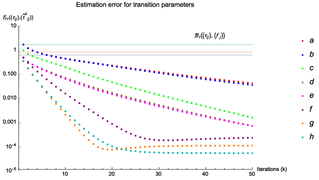
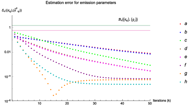
For each set of pairs of activity functions in Table 1 we run the algorithm for $50$ iterations. Figures 1 and 2 plot the averaged relative entropy for the parameter estimates as a function of iteration step. The labels (a)–(h) to the right of each plot appear in the order of the final error values. We do not provide a plot showing convergence of $(\hat{\pi}^{k}_{j})$ since the only noticeable trend is that if they converge to an exact state value, it is usually to the initial state of the interpolated sequence $z$ .

In each case the error for both the transitions and the emissions decreases to small values. Since the $\mathsf{ARE}$ depends on the activity functions as well as on the parameters and their estimates, we need to compute a baseline error value for each case. For the parameters $(\tau_{ij})$ and a specific choice of $(f_{j})$ it is:

\mathcal{B}_{\tau}\big((\tau_{ij}),(f_{j})\big)=\mathsf{E}\Big[\mathsf{ARE}\Big(\big(a_{ij}(t)\big),\big(a^{\prime}_{ij}(t)\big)\Big)\Big],

where $a_{ij}(t)$ and $a^{\prime}_{ij}(t)$ are related through $f_{j}$ to $\tau_{ij}$ and $\tau^{\prime}_{ij}$ , respectively, by eq. (1), and where $\mathsf{E}[\cdot]$ denotes the expectation over uniformly random $(\tau^{\prime}_{ij})$ . To estimate this expectation value, we compute the average $\mathsf{ARE}$ of the parameters with respect to 1000 independently chosen sets of random parameters (rather than their estimates from our algorithm), for each case (a)–(h). For the emission parameters we compute baselines the same way, using 1000 uniformly random values $(\epsilon^{\prime}_{sj})$ to estimate

\mathcal{B}_{\epsilon}\big((\epsilon_{sj}),(g_{j})\big)=\mathsf{E}\Big[\mathsf{ARE}\Big(\big(b_{sj}(t)\big),\big(b^{\prime}_{sj}(t)\big)\Big)\Big],

where $b_{sj}(t)$ and $b^{\prime}_{sj}(t)$ are related through $g_{j}$ to $\epsilon_{sj}$ and $\epsilon^{\prime}_{sj}$ , respectively, by eq. (3), and where $\mathsf{E}[\cdot]$ denotes the expectation value over uniformly random $(\epsilon^{\prime}_{sj})$ . The baseline averages thus obtained for function pairs in Table 1 are recorded in Table 2, where the row labels indicate the parameters being baselined.

o—[1.5pt]c—[1.5pt]c—c—c—c—c—c—c—c—[1.5pt]	a	b	c	d	e	f	g	h
$\mathcal{B}_{\tau}\big((\tau_{ij}),(f_{j})\big)$	$1.637$	$1.677$	$1.657$	$0.615$	$0.603$	$0.811$	$0.81$	$0.610$
$\mathcal{B}_{\epsilon}\big((\epsilon_{sj}),(g_{j})\big)$	$0.603$	$0.578$	$1.563$	$0.592$	$0.584$	$1.466$	$1.539$	$1.534$

Table 2. Baseline errors for

(\tau_{ij})

and

(\epsilon_{sj})

for activity function pairs from Table 1.

We plot these baseline errors as horizontal lines in Figures 1 and 2. Most of these are too close to be distinguishable; indeed they are all $O(1)$ , in contrast to the estimation errors plots which are almost all smaller by at least an order of magnitude, and in most cases by 3 or 4, indicating very good parameter estimates. Furthermore, the relative quality of the estimates can be understood: Case (c) is the standard HMM, for which our algorithm reduces to the Baum-Welch algorithm [1, 17]. Cases (a) and (b) have greater errors, which is not surprising since they have non-constant emission activity functions, oscillating in value up to 1. This means that for each of these cases, non-zero emissions are lower probability events, so there is less information in $y$ . Possibly surprising is the fact that when the transition activity function is non-constant, cases (d)–(h), the errors are smaller than in the standard HMM case. But this happens because state changing transitions are reduced, so that each non-zero emission observed provides more information. And among these cases, those with varying emission activity levels have larger errors than those without.

Refer to caption — Figure 1. Transition parameters estimation error, $\mathcal{E}_{\tau}\big((\tau_{ij}),(\hat{\tau}^{k}_{ij})\big)$ , for successive iterations $k$ . Labels to the right are of activity function pairs from Table 1, and are displayed in the order of the final error values. Baseline errors, $\mathcal{B}_{\tau}\big((\tau_{ij}),(f_{j})\big)$ , from Table 2 are shown as horizontal lines.

References

[1] L. E. Baum and J. A. Eagon (1967) An inequality with applications to statistical estimation for probabilistic functions of markov processes and to a model for ecology. Bulletin of the American Mathematical Society 73, pp. 360–363. Cited by: §1, §3.
[2] S. Çolak, L. P. Alexander, B. G. Alvim, S. R. Mehndiretta, and M. C. González (2015) Analyzing cell phone location data for urban travel: current methods, limitations and opportunities. In Transportation Research Board 94th Annual Meeting, pp. 17. Cited by: §1.
[3] B. Cs. Csáji, A. Browet, V. A. Traag, J.-C. Delvenne, E. Huens, P. Van Dooren, Z. Smoreda, and V. D. Blondel (2013) Exploring the mobility of mobile phone users. Physica A 392, pp. 1459–1473. Cited by: §1.
[4] A. P. Dempster, N. M. Laird, and D. B. Rubin (1977) Maximum likelihood from incomplete data via the em algorithm. Journal of the Royal Statistical Society, Series B 39, pp. 1–38. Cited by: §1.
[5] L. Deng (1993) A stochastic model of speech incorporating hierarchical nonstationarity. IEEE Transactions on Speech and Audio Processing 1, pp. 471–474. Cited by: §1.
[6] R. W. Douglass, D. A. Meyer, M. Ram, D. Rideout, and D. Song (2015) High resolution population estimates from telecommunications data. EPJ Data Science 4, pp. pp. 13. Cited by: §1.
[7] J. D. Ferguson (1980) Variable duration models for speech. In Proceedings of the Symposium on the Application of HMMs to Text and Speech, pp. 143–179. Cited by: §1.
[8] J.-M. François, G. Leduc, and S. Martin (2004) Learning movement patterns in mobile networks: a generic method. In European Wireless, pp. 128–134. Cited by: §1.
[9] M. C. González, C. A. Hidalgo, and A.-L. Barabási (2008) Understanding individual human mobility patterns. Nature 453, pp. 779–782. Cited by: §1.
[10] R. Kitamura, C. Chen, R. M. Pendyala, and R. Narayanan (2000) Micro-simulation of daily activity-travel patterns for travel demand forecasting. Transportation 27, pp. 25–51. Cited by: §1.
[11] P. Lanchantin and W. Pieczynski (2004) Unsupervised non-stationary image segmentation using triplet markov chains. In Proceedings of the Advanced Concepts for Intelligent Vision Systems (ACIVS 04), pp. 6. Cited by: §1.
[12] M. Lenormand, T. Louail, O. G. Cantu-Ros, M. Picornell, R. Herranz, J. M. Arias, M. Barthelemy, M. San Miguel, and J. J. Ramasco (2014) Influence of sociodemographic characteristics on human mobility. arXiv:1411.7895v1 [physics.soc-ph]. Cited by: §1.
[13] W. Mathew, R. Raposo, and B. Martins (2012) Predicting future locations with hidden markov models. In Proceedings of the ACM Conference on Ubiquitous Computing, pp. 911–918. Cited by: §1.
[14] T. A. Perkins, A. J. Garcia, V. A. Paz-Soldán, S. T. Stoddard, R. C. Reiner, Jr.,, G. Vazquez-Prokopec, D. Bisanzio, A. C. Morrison, E. S. Halsey, T. J. Kochel, D. L. Smith, U. Kitron, T. W. Scott, and A. J. Tatem (2014) Theory and data for simulating fine-scale human movement in an urban environment. Journal of the Royal Society Interface 11, pp. 20140642, pp. 12. Cited by: §1.
[15] B. Sin and J. H. Kim (1995) Nonstationary hidden markov model. Signal Processing 46, pp. 31–46. Cited by: §1.
[16] C. Song, Z. Qu, N. Blum, and A.-L. Barabási (2010) Limits of predictability in human mobility. Science 327, pp. 1018–1021. Cited by: §1.
[17] L. R. Welch (2003) Hidden markov models and the baum-welch algorithm. IEEE Information Theory Society Newsletter 53 (1), pp. 10–13. Cited by: §1, §3.