Lagrangian coherent structures and plasma transport processes

M. V. Falessi\aff1 \corresp Email: falessi@fis.uniroma3 F. Pegoraro\aff2 T. J. Schep\aff3 Affiliation: \aff1 Dipartimento di Matematica e Fisica, Roma Tre University, Via della Vasca Navale 84, 00199 Roma, Italy \aff2Dipartimento di Fisica, Pisa University, Largo Bruno Pontecorvo 3, 56127 Pisa, Italy \aff3Department of Physics, Eindhoven University of Technology, De Rondom 70,5612 AP Eindhoven, Netherlands

Abstract

A dynamical system framework is used to describe transport processes in plasmas embedded in a magnetic field. For periodic systems with one degree of freedom the Poincaré map provides a splitting of the phase space into regions where particles have different kinds of motion: periodic, quasi-periodic or chaotic. The boundaries of these regions are transport barriers; i.e., a trajectory cannot cross such boundaries during the whole evolution of the system. Lagrangian Coherent Structure (LCS) generalize this method to systems with the most general time dependence, splitting the phase space into regions with different qualitative behaviours. This leads to the definition of finite-time transport barriers, i.e. trajectories cannot cross the barrier for a finite amount of time. This methodology can be used to identify fast recirculating regions in the dynamical system and to characterize the transport between them.

1 Introduction

Transport phenomena are ubiquitous in nature and involve the redistribution of physical quantities such as mass, charge, linear and angular momentum and energy etc. Different mechanisms are at work in the transport processes ranging from diffusion to advection and mixing in the case of turbulent or chaotic motions. Recently a new concept in the study of transport processes in complex fluid flows was introduced by Peacock & Haller (2013): Lagrangian coherent structures (LCS). In a two-dimensional configuration these structures are special lines¹¹ 1 In the most general system the LCS are surfaces advected by the flow but here for the sake of simplicity we will only deal with $2D$ systems. advected by the fluid which organize the flow transport processes by attracting or repelling the nearby fluid elements over a finite time span. Strictly speaking we should call these structures Hyperbolic LCS. Two other kinds of LCS have been introduced in the literature. For the definition of all the different kinds of LCS we indicate the recent review by Haller (2015). For the sake of simplicity we will refer to these structures simply as LCS. These special lines organise the flow splitting the domain into macro-regions with fast mixing phenomena inside them. Over the finite time span which characterizes the LCS these macro regions do not exchange fluid elements. The LCS have been widely used in the literature to characterize transport processes in various systems: the pollutant transport on the ocean surface (Coulliette et al., 2007), blood flow (Shadden & Taylor, 2008), the spreading of plankton blooms (Huhn et al., 2012), turbulent combustion (Hamlington et al., 2011), jellyfish predator-prey interaction (Peng & Dabiri, 2009), atmospheric dataset analysis (Tang et al., 2010), solar photospheric flows (Chian et al., 2014), saturation of a nonlinear dynamo (Rempel et al., 2013), etc.

Plasmas are often studied using “fluid” theories either in phase space, such as the Vlasov-Maxwell system, or in physical space such as the two fluid and the MHD systems. The LCS techniques can therefore be applied to study transport processes, i.e. the mixing of fluid elements, in these systems. In (citation to another proceeding: Carlevaro, Falessi, Montani, Zonca) the LCS has been used to quantify the phase space transport due to the interactions between two supra-thermal electron beams and a cold, homogeneous, background plasma. In two recent works (Borgogno et al., 2011a; Borgogno et al., 2011b) it was shown how the LCS can provide information about the electron transport due to the stochastization of the magnetic field in a collisionless reconnection process.

The introduction of these techniques is relatively recent and, in spite of their increasing use, their rigorous definition has been subject to debate (Shadden et al., 2005; Haller, 2011). The first definitions of an LCS were based on the Finite time Lyapunov exponent profile. These have been shown to be incorrect by G.Haller who found several counterexamples to this heuristic definition. The rigorous definition of an LCS as the most repulsive or attractive material line with respect to the nearby ones was introduced by (Haller, 2011). In this article we provide a simplified version of this derivation in order to give to the reader some physical intuition about these structures, we analytically calculate the shape of the LCS in a simple Hamiltonian system and, finally, we compare the LCS obtained by Borgogno et al. (2011a) using the FTLE method with the ones obtained with the rigorous definition introduced. The numerical framework used to compute the LCS shape was developed by Onu et al. (2015).

2 Lagrangian Coherent Structures and Transport Barriers

2.1 Lagrangian Coherent Structures as most repelling material lines

Following (Haller, 2011), in this section we briefly review some mathematical concepts that lead to the definition of LCS.

We consider a dynamical system in 2D phase space ${\bf x}=(x,y)$ ,

\frac{d{x}}{dt}={v_{x}}(t,{x,y}),\qquad\frac{d{y}}{dt}={v_{y}}(t,{x,y})

(1)

with continuous differentiable flow map

{\boldsymbol{\phi}}_{t_{0}}^{t}({\bf{\boldsymbol{x}}_{0}})={\bf x}(t,t_{0},{\bf{\boldsymbol{x}}_{0}}).

(2)

Two neighbouring points ${\bf x}_{0}$ and ${\bf x}_{0}+\delta{\bf x}_{0}$ evolve into the points ${\bf x}$ and ${\bf x}+\delta{\bf x}$ under the linearized map

|\delta x\rangle={\boldsymbol{\nabla}}{\boldsymbol{\phi}}_{t_{0}}^{t}\,|\delta{x}_{0}\rangle.

(3)

where for notational convenience, we adopt a bra-ket notation for vectors and scalar products and represent a generic column vector as $|c\rangle$ and a row vector as $\langle r|$ . Their scalar product is denoted as $d=\langle c|r\rangle$ .

Consider a curve $\gamma_{0}=\{{\bf x}_{0}=r(s)\}$ . At each point ${\boldsymbol{x}}_{0}\in\gamma_{0}$ , define the unit tangent vector $|e_{0}\rangle$ and the normal vector $|n_{0}\rangle$ . In the time interval $[t_{0},t]$ the dynamics of the system advects the “material line” $\gamma_{0}$ into $\gamma_{t}$ and ${\boldsymbol{x}}_{0}\in\gamma_{0}$ into ${\boldsymbol{x}}_{t}\in\gamma_{t}$ . The linearized dynamics maps the tangent vector $\left|e_{0}\right\rangle$ into $\left|e_{t}\right\rangle$ which is tangent to $\gamma_{t}$

|e_{t}\rangle=\frac{\boldsymbol{\nabla}{\boldsymbol{\phi}}^{t}_{t_{0}}({\boldsymbol{x}}_{0})|e_{0}\rangle}{\sqrt{\left\langle e_{0}\left|\left(\boldsymbol{\nabla}{\boldsymbol{\phi}}^{t}_{t_{0}}\right)^{T}\boldsymbol{\nabla}{\boldsymbol{\phi}}^{t}_{t_{0}}\right|e_{0}\right\rangle}}\equiv\frac{\boldsymbol{\nabla}{\boldsymbol{\phi}}^{t}_{t_{0}}({\boldsymbol{x}}_{0})|e_{0}\rangle}{\sqrt{\left\langle e_{0}\left|C^{t}_{t_{0}}({\boldsymbol{x}}_{0})\right|e_{0}\right\rangle}},

(4)

where $C^{t}_{t_{0}}({\boldsymbol{x}}_{0})\equiv\left(\boldsymbol{\nabla}{\boldsymbol{\phi}}^{t}_{t_{0}}\right)^{T}\,\boldsymbol{\nabla}{\boldsymbol{\phi}}^{t}_{t_{0}}$ is the Cauchy-Green strain tensor and ^T stands for transposed. This symmetric tensor describes the deformation of an arbitrarily small circle of initial conditions, centered in ${\boldsymbol{x}}_{0}$ caused by the flow in a time interval $[t_{0},t]$ . As an example let us consider a circle centered in ${\boldsymbol{x}}_{0}$ with radius $\|\delta{\boldsymbol{x}}_{0}\|$ . After the time interval $[t_{0},t]$ this will be deformed into an ellipse with major axis in the direction of $\left|\xi_{max}\right\rangle$ and minor axis in the direction of $\left|\xi_{min}\right\rangle$ being $\left|\xi_{max}\right\rangle$ and $\left|\xi_{min}\right\rangle$ the two eigenvectors of $C^{t}_{t_{0}}({\boldsymbol{x}}_{0})$ . The corresponding real and positive eigenvalues are $\lambda_{max}$ and $\lambda_{min}$ . The length of the major axis is $\lambda_{max}\|{\delta}{\boldsymbol{x}}_{0}\|$ while the the length of the minor is $\lambda_{min}\|\delta{\boldsymbol{x}}_{0}\|$ . The curves with tangent vector along $\left|\xi_{min}\right\rangle$ and, respectively, $\left|\xi_{max}\right\rangle$ are called strain lines of the Cauchy-Green tensor. In general, the mapping will not preserve the angle between vectors and therefore usually $\left|n_{t}\right\rangle$ differs from $\boldsymbol{\nabla}{\boldsymbol{\phi}}^{t}_{t_{0}}\left|n_{0}\right\rangle$ .

Using the condition $\left\langle n_{0}|e_{0}\right\rangle=\left\langle n_{0}\left|\boldsymbol{\nabla}{\boldsymbol{\phi}}^{t_{0}}_{t}\boldsymbol{\nabla}{\boldsymbol{\phi}}^{t}_{t_{0}}\right|e_{0}\right\rangle$ =0 and inserting Eq. (4) we obtain the expression for $\left|n_{t}\right\rangle$ which is given by

|n_{t}\rangle=\frac{\left(\boldsymbol{\nabla}{\boldsymbol{\phi}}^{t_{0}}_{t}\right)^{T}|n_{0}\rangle}{\sqrt{\left\langle n_{0}\left|\boldsymbol{\nabla}{\boldsymbol{\phi}}^{t_{0}}_{t}\left(\boldsymbol{\nabla}{\boldsymbol{\phi}}^{t_{0}}_{t}\right)^{T}\right|n_{0}\right\rangle}}\equiv\frac{\left(\boldsymbol{\nabla}{\boldsymbol{\phi}}^{t_{0}}_{t}\right)^{T}|n_{0}\rangle}{\sqrt{\left\langle n_{0}\left|C^{-1}({\boldsymbol{x}}_{0})\right|n_{0}\right\rangle}},

(5)

where $C^{-1}({\boldsymbol{x}}_{0})=C^{t_{0}}_{t}({\boldsymbol{x}}_{0})$ and the time interval marks have been suppressed as will be the case in the following formulae when not explicitly needed. We define the repulsion ratio $\rho^{t}_{t_{0}}({\boldsymbol{x}}_{0},n_{0})$ as the ratio at which material points, in other words points advected by the flow, initially taken near the point ${\boldsymbol{x}}_{0}\in\gamma_{0}$ , increase their distance from the curve in the time interval $[t_{o},t]$ :

\rho^{t}_{t_{0}}({\boldsymbol{x}}_{0},n_{0})=\left\langle n_{t}\left|\boldsymbol{\nabla}{\boldsymbol{\phi}}^{t}_{t_{0}}({\boldsymbol{x}}_{0})\right|n_{0}\right\rangle.

(6)

In order to understand this definition we may imagine measuring the distance between ${\boldsymbol{x}}_{0}$ , taken on the curve $\gamma_{0}$ , and a point initially placed at unit distance from the curve. After a sufficiently small amount of time this distance is measured by the projection of the vector $\boldsymbol{\nabla}{\boldsymbol{\phi}}^{t}_{t_{0}}({\boldsymbol{x}}_{0})|n_{0}\rangle$ along $\left|n_{t}\right\rangle$ as shown in Figure 1.

Refer to caption — Figure 1: The green line and the purple line represent the trajectories of two elements of the system. The continuous thick black line is the curve $\gamma_{0}$ while the dashed one is its evolution $\gamma_{t}$ at time $t$ . We have marked in blue the evolution of $\left|n_{0}\right\rangle$ through the linearized dynamic and in red its projection on $\left|n_{t}\right\rangle$ .

Using the previous definitions, $\rho^{t}_{t_{0}}({\boldsymbol{x}}_{0},n_{0})$ can be expressed either in terms of $n_{0}$ or of $n_{t}$ as

\rho^{t}_{t_{0}}({\boldsymbol{x}}_{0},n_{0})=\frac{1}{\sqrt{\left\langle n_{0}\left|C^{-1}({\boldsymbol{x}}_{0})\right|n_{0}\right\rangle}}=\sqrt{\left\langle n_{t}\left|C({\boldsymbol{x}}_{0})\right|n_{t}\right\rangle}.

(7)

Similarly, the contraction rate $L^{t}_{t_{0}}({\boldsymbol{x}}_{0})$ is proportional to the growth in time of the vector tangent to the material line

L({\boldsymbol{x}}_{0},e_{0})=\sqrt{\left\langle e_{0}\left|C({\boldsymbol{x}}_{0})\right|e_{0}\right\rangle}.

(8)

The aim in these definitions is to characterize a LCS over a finite time interval $\left[t_{0},t_{0}+T\right]$ as a material line, in other words a curve advected by the flow, which is locally the strongest repelling or attracting curve with respect to the nearby ones. This leads, as shown by Haller (2011), to the following definitions.

Definition 1

A material line satisfying the following conditions at each point:

1.

$\lambda_{min}<\lambda_{max},\quad\lambda_{max}>1$ (9)
2.

the tangent vector is along the eigenvector associated with the smallest eigenvalue

$\left|e_{0}\right\rangle=\left|\xi_{min}\right\rangle,$ (10)
3.

the gradient of the largest eigenvalue is along the curve

$\left\langle\xi_{max}\Big|\nabla\lambda_{max}\right\rangle=0$ (11)

is called a Weak Lagrangian coherent structure (WLCS).

Definition 2

A WLCS which satisfies the following additional condition

1.

at each point the relationship

$\left\langle\xi_{max}\left|\nabla^{2}\lambda_{max}\right|\xi_{max}\right\rangle<0$ (12)

holds is called a Lagrangian coherent structure.

A simplified illustration of the previous conditions can be given as follows. The first condition is obtained when requiring that at each point ${\boldsymbol{x}}_{0}$ of the material line the repulsion rate $\rho({\boldsymbol{x}}_{0},n_{0})$ is larger than the contraction rate $L({\boldsymbol{x}}_{0},n_{0})$ which represents the effect of the shear along the material line. At each point along a material line the tangent vector can be expressed in terms of the eigenvectors $\left|\xi_{min}\right\rangle$ and $\left|\xi_{max}\right\rangle$ of the Cauchy-Green strain tensor $C$ :

\left|e_{0}\right\rangle=\alpha\left|\xi_{min}\right\rangle+\beta\left|\xi_{max}\right\rangle,\quad\alpha^{2}+\beta^{2}=1.

(13)

where $\alpha$ and $\beta$ represent the orientation of the material line and may be arbitrary functions of ${\boldsymbol{x}}_{0}$ . It follows that

\left|n_{0}\right\rangle=\alpha\left|\xi_{max}\right\rangle-\beta\left|\xi_{min}\right\rangle.

(14)

We can therefore express the repulsion rate in terms of $\alpha$ and $\beta$

\rho^{t}_{t_{0}}({\boldsymbol{x}}_{0},n_{0})=\frac{1}{\sqrt{\left\langle n_{0}\left|C^{-1}\right|n_{0}\right\rangle}}=\left(\frac{\alpha^{2}}{\lambda_{max}}+\frac{\beta^{2}}{\lambda_{min}}\right)^{-1/2}.

(15)

Now at each point ${\boldsymbol{x}}_{0}$ we maximize $\rho^{t}_{t_{0}}$ with respect to the direction of the tangent vector $\left|e_{0}\right\rangle$ i.e., of the orientation of the chosen material line, with the constraint $\alpha^{2}+\beta^{2}=1$ . This yields $\alpha=1$ , $\beta=0$ , so that

\rho^{t}_{t_{0}}=\sqrt{\lambda_{max}},

(16)

which implies that the material line must be chosen to be the strain line oriented along the eigenvector $\left|\xi_{min}\right\rangle$ as required by Eq. (10). At this stage we need to maximize the repulsion rate along the material line with respect to nearby material lines. Therefore we define

R^{t}_{t_{0}}(\gamma_{0})\equiv\int_{s_{1}}^{s_{2}}ds\,\rho\left({\boldsymbol{x}}_{0}(s),n_{0}(s)\right),

(17)

which has the physical meaning of the repulsion rate integrated over a curve $\gamma_{0}$ . We consider a curve $\gamma_{\epsilon}$ with points ${\boldsymbol{x}}_{\epsilon}\in\gamma_{\epsilon}$ such that

{\boldsymbol{x}}_{\epsilon}={\boldsymbol{x}}_{0}+\epsilon h(s)\left|n_{0}\right\rangle.

(18)

The first variation of Eq. (17) with respect to Eq. (18) gives

\delta R^{t}_{t_{0}}(\gamma_{\epsilon})[h]=\delta\int_{s_{1}}^{s_{2}}ds\,\rho\left(x_{\epsilon}(s),n_{\epsilon}(s)\right)=0,

(19)

which can be computed as

\lim_{\epsilon\to 0}\frac{\partial}{\partial\epsilon}\int_{s_{1}}^{s_{2}}ds\rho\left(x_{\epsilon}(s),n_{\epsilon}(s)\right)=\lim_{\epsilon\to 0}\frac{\partial}{\partial\epsilon}\int_{s_{1}}^{s_{2}}ds\sqrt{\lambda_{max}\left(x_{\epsilon}(s),n_{\epsilon}(s)\right)}

(20)

leading to

\delta R^{t}_{t_{0}}(\gamma_{\epsilon})[h]=\int_{s_{1}}^{s_{2}}\frac{ds\,h(s)}{2\sqrt{\lambda_{max}}}\left\langle\left.\boldsymbol{\nabla}\lambda_{max}\right|\xi_{max}\right\rangle=0

(21)

which vanishes if $\left|\boldsymbol{\nabla}\lambda_{max}\right\rangle$ is tangent to the material line. Requiring that this material line represents a maximum of the integrated repulsion rate we obtain

\left\langle\xi_{max}\left|\nabla^{2}\lambda_{max}\right|\xi_{max}\right\rangle<0

(22)

which is the condition that defines the locally most repelling LCSs. These structures are Lagrangian by definition and have no transport through them because they are material lines.

2.2 Lagrangian Coherent Structures as second derivative ridges

Second derivative ridges were defined by Shadden et al. (2005) in terms of the features of the Lyapunov exponent field $\sigma({\boldsymbol{x}}_{0},t_{0},t)$ that characterizes the rate of separation of close trajectories.

The finite time Lyapunov exponent can be expressed in terms of the Cauchy-Green tensor eigenvalues as

\sigma({\boldsymbol{x}}_{0},t_{0},t)=\frac{1}{2|t-t_{0}|}\,\ln{\lambda_{max}}({\boldsymbol{x}}_{0},t_{0},t)

(23)

Definition 3

Curves ${\boldsymbol{r}}(s)$ (not necessarily material lines) such that

1.

the tangent vector $\left|r^{\prime}(s)\right\rangle$ and $\,{\boldsymbol{\nabla}}\sigma$ along the curve are parallel,
2.

the normal unit vector $\left|n\right\rangle$ is such that along the curve for all $\left\langle u|u\right\rangle=1$

$\left\langle n\left|\Sigma\right|n\right\rangle={\rm min}\,|_{\langle u|u\rangle=1}\left\langle u\left|\Sigma\right|u\right\rangle<0$ (24)

where $\Sigma$ is the Hessian matrix of the second derivatives of $\sigma$ with respect to ${\boldsymbol{x}}_{0}$ is called a second derivative ridge.

A major difference between the two sets of definitions is that the most repelling LCS definition involves the eigenvectors and eigenvalues of the Cauchy-Green strain tensor, while the second condition in the definition of the second derivative ridge is governed by the eigenvectors and eigenvalues of the matrix $\Sigma$ .

3 Example: a Hamiltonian flow map

In this section we will illustrate the definitions introduced above and the procedure needed in order to identify and characterize the Lagrangian coherent structures by direct construction in a simplified dynamical system that can be studied analytically. We find it convenient to consider a Hamiltonian system which ensures condition (9) through conservation of phase space volume. We consider the time independent Hamiltonian

H=\frac{x^{2}y}{2},

(25)

from which we obtain

\left\{\begin{array}[]{ll}\frac{dx}{dt}=-\frac{x^{2}}{2}\\ \frac{dy}{dt}=xy\par\end{array}\right.

(26)

A contour plot of the Hamiltonian $H$ is given in Fig. 2. The trajectories obtained by integrating Eq. (26) coincide with the lines of constant $H$ .

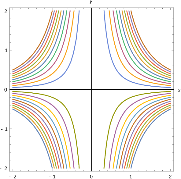
Integrating the system (26) we obtain

	$\displaystyle x(t)=\left({\boldsymbol{\phi}}_{0}^{t}({x}_{0},y_{0})\right)_{x}$	$\displaystyle=$	$\displaystyle\frac{2{x}_{0}}{2+{x}_{0}t}$		(27)
	$\displaystyle y(t)=\left({\boldsymbol{\phi}}_{0}^{t}({x}_{0},y_{0})\right)_{y}$	$\displaystyle=$	$\displaystyle y_{0}\left(1+\frac{{x}_{0}t}{2}\right)^{2},$		(28)

where ${x}_{0}=x(t=0)$ and $y_{0}=y(t=0)$ . From Eq. (27) we see that points with negative ${x}_{0}$ reach $x=-\infty$ in a finite time while points with positive ${x}_{0}$ reach $x=0$ for $t\to\infty$ . In order to avoid this finite time singularity we restrict the domain to the semi-plane ${x}_{0}>0$ .
The matrix $\nabla{\boldsymbol{\phi}}^{t}_{0}$ takes the form

\nabla{\boldsymbol{\phi}}_{0}^{t}=\left(\begin{array}[]{cc}{1}/{B^{2}}&0\\ {B}ty_{0}&{B^{2}}\end{array}\right)

(29)

where $B=1+t{x}_{0}/2$ . The Cauchy Green strain tensor $C_{0}^{t}({x}_{0},y_{0})\equiv\left(\nabla{\boldsymbol{\phi}}_{0}^{t}\right)^{T}\,\nabla{\boldsymbol{\phi}}_{0}^{t}$ is

C_{0}^{t}({x}_{0},y_{0})=B^{2}\left(\begin{array}[]{cc}{1}/{B^{6}}+\left({ty_{0}}\right)^{2}&\,\,\,\,B{ty_{0}}\\ B{ty_{0}}&\,\,\,\,B^{2}\end{array}\right).

(30)

In order to identify its eigenvectors and corresponding eigenvalues it may be convenient to diagonalize it

R({\varphi})\,\,C^{t}_{0}\,\,R^{T}({\varphi})=D.

(31)

by means of the rotation $R({\varphi})$

R({\varphi})=\left(\begin{array}[]{cc}\cos{\varphi}&\,\,\,\,-\sin{\varphi}\\ \sin{\varphi}&\,\,\,\,\cos{\varphi}\end{array}\right)

(32)

with ${\varphi}$ given by

{\varphi}=\frac{1}{2}\arctan\left(\frac{2Bty_{0}}{{B}^{2}-1/B^{6}-(ty_{0})^{2}}\right)

(33)

and $D({x}_{0},y_{0})$ is the diagonal matrix

D=\left(\begin{array}[]{cc}\lambda_{min}&\,\,\,\,0\\ 0&\,\,\,\,\lambda_{max}\end{array}\right)

(34)

with $\lambda_{max}=\lambda_{+}$ , $\lambda_{min}=\lambda_{-}$ and

\lambda_{\pm}=\frac{1+B^{8}+B^{6}t^{2}y_{0}^{2}\pm\sqrt{\left[1+B^{8}+B^{6}t^{2}y_{0}^{2}\right]^{2}-4B^{8}}}{2\,B^{4}}.

(35)

The rotation angle $\varphi({x}_{0},y_{0})$ can be used to find the orientation of the strain lines. Note that $\varphi(x_{0},y_{0}=0)=0$ , as the strain tensor in Eq. (30) is diagonal on the positive semi axis $y_{0}=0$ with $|\xi_{\min}\rangle$ tangent this axis i.e., in the $x_{0}$ direction. In fact from Eqs. (27) we see that if we take two points $x_{01}$ and $x_{02}$ on the positive $y_{0}=0$ semi-axis, with $x_{02}>x_{01}$ they stay on this axis and their distance $d(t)$ decreases in time:

d(t)=\frac{d(0)}{1+t\left(x_{02}+x_{01}\right)/2+t^{2}x_{02}x_{01}/4},

(36)

as consistent with the fact that this $y_{0}=0$ axis is parallel to $|\xi_{\min}\rangle$ at all times. In order to show the strain lines of the Cauchy-Green tensor for $x_{0}>0$ in Fig. 3 we plot the vector fields $|\xi_{max}\rangle=R^{T}({\varphi})|0,1\rangle=|(\sin{\varphi},\cos{\varphi})\rangle$ and $|\xi_{min}\rangle=R^{T}({\varphi})|1,0\rangle=|\cos{\varphi},-\sin{\varphi})\rangle$ in the limit of sufficiently long times such that $tx_{0}\gg 2$ in which limit the rotation angle $\varphi$ reduces to:

{\varphi}\sim(1/2)\arctan[(x_{0}y_{0})/(y_{0}^{2}-x_{0}^{2}/4)]=\arctan\frac{2y_{0}}{x_{0}}

(37)

and becomes independent of time.

In the same limit the eigenvalues of the Cauchy-Green strain tensor become simply

\lambda_{max}\sim{t^{4}}\left(x_{0}^{4}+4y_{0}^{2}{x}_{0}^{2}\right)/16,\qquad\lambda_{min}=1/\lambda_{max}

(38)

and have a factorized time and space dependence.

From (38) we can compute ${\boldsymbol{\nabla}}\lambda_{max}$ (which will be parallel to ${\boldsymbol{\nabla}}\lambda_{min}$ )

{\boldsymbol{\nabla}}\lambda_{max}=\frac{t^{4}x_{0}}{4}\left(\begin{array}[]{cc}x_{0}^{2}+2y_{0}^{2}\\ 2x_{0}y_{0}\end{array}\right)\quad\propto\cos{\varphi}\left(\begin{array}[]{cc}\cos^{2}{\varphi}+2\sin^{2}{\varphi}\\ 2\cos{\varphi}\sin{\varphi}\end{array}\right).

(39)

A contour plot of Eq. (38) is shown in Figure 4.

Recalling the sufficient and necessary condition in order to have a WLCS is $\left\langle\xi_{max}\Big|\nabla\lambda_{max}\right\rangle=0$ we find the condition $\cos{\varphi}\,\sin{\varphi}\,(2\sin^{2}{\varphi}+3\cos^{2}{\varphi})=0$ . For $x_{0}\not=0$ (i.e $\varphi\not=\pi/2$ ), this condition implies $\sin{\varphi}=0$ . Thus the only repulsive WLCS is given by the positive $y_{0}=0$ semi-axis.

It is easy to see that the condition (12) is not satisfied, i.e., this WLCS is not a maximum for the repulsive rate and thus is not an LCS.

Referring now to the definition of the second derivative ridges, from 38 at $y_{0}=0$ we find

\Sigma(x_{0},y_{0}=0)=\frac{4}{x_{0}^{2}}\left(\begin{array}[]{cc}-1&\,\,\,\,0\\ \,\,0&\,\,\,\,2\end{array}\right)

(40)

which is not negative definite and for which $\left\langle n\left|\Sigma\right|n\right\rangle$ is a maximum, not a minimum, contrary to the requirement (24) in the second derivative ridge definition.

In this example the WLCS according to Haller’s definition that we found at $y_{0}=0$ is not a second derivative ridge.

4 Electron transport in a 3D reconnection process

In this section we will deal with the barriers to the transport of electrons in a $3$ D magnetic reconnection processes in the presence of a fixed “guide field” component $B_{z}$ . A simplified doubly-periodic slab geometry is considered. Because of this double periodicity this model can be applied mainly to toroidal thermonuclear plasmas (Borgogno et al., 2005; Avinash et al., 1998; Porcelli et al., 2002), and with some modification to space plasmas (Rappazzo & Parker, 2013) and, more generally, to physical contexts where plasma is confined by a nearly uniform strong magnetic field with small perturbations. Under proper adiabaticity conditions, and in particular assuming that their Larmor radius is negligible, charged particles move along magnetic field lines. Therefore in this approximation the study of the motion of electrons can be referred to the study of the topology of the magnetic field lines.

The magnetic field structure and evolution are described through the evolution of the magnetic flux function $\psi(x,y,z,t)$ by the relationship

{\bf B}=B_{0}{\bf e}_{z}+{\bf e}_{z}\times\nabla\psi.

(41)

As for all solenoidal fields in an odd dimensional space, at any fixed time $t={\bar{t}}$ the magnetic field line equations can be written in the form of Hamilton’s equations. The function $\psi(x,y,z,{\bar{t}})$ plays the role of the Hamiltonian while the coordinate $z$ plays the role of the time variable in this Hamiltonian system. Using a periodic geometry along $z$ allows us to study the shape of magnetic field lines with dynamical systems techniques such as the Poincaré map. The growth and interaction of different unstable modes will naturally lead to the formation of structures in the magnetic field such as magnetic islands and to chaotic behaviour of field lines. Assuming, as commonly done, that the time it takes electrons to complete a number of turns along $z$ before the magnetic field is significantly changed, we can investigate the advection of particles in such a chaotic system at a fixed $t={\bar{t}}$ using the LCS technique. This requires that the electron thermal velocity be sufficiently larger than the Alfvèn speed and allows us to highlight the finite time transport barriers of the system. Choosing the LCS characteristic time span $\left|z-z_{0}\right|$ properly, we obtain the boundaries of the regions where fast electron mixing is expected. After a time span of the order of the Alfvén time we can expect that the shape of the magnetic field lines will have changed significantly and therefore we need to “refresh” the Hamiltonian $\psi(x,y,z,{\bar{t}})$ and plot a new Poincaré map for the magnetic field. The LCS of the Poincaré map calculated with a sufficient number of iterations marks the boundaries of the regions where the electrons will mix.

In this paper we will not deal with the numerical integration of the PDE governing the dynamics. We will instead study the shape of the magnetic field lines at fixed $t$ extracting $\psi$ from the numerical simulation carried out by Borgogno et al. (2005). An analogue analysis has been carried out by Borgogno et al. (2011a) where the LCS have been calculated using the definition based on the ridges of the Finite time Lyapunov exponent field. We choose the same values for the parameters defining the LCS in order to make a comparison with this work.

4.1 The physical system

The physical system studied is a Hamiltonian reconnection process in a dissipationless 3D plasma immersed in a strong, uniform, externally imposed magnetic field. A slab geometry is used with a formal additional periodicity along $x$ imposed for numerical convenience. The algorithm applied in the numerical simulation is detailed in Borgogno et al. (2008). The reconnection process develops in a static equilibrium configuration given by:

\psi_{eq}(x)=A\cos(x),

(42)

with $A=0.19$ . The integration domain is defined by $-L_{x}<x<L_{x}$ , $-L_{y}<y<L_{y}$ , $-L_{z}<z<L_{z}$ with $L_{x}=\pi$ , $L_{y}=2\pi$ and $L_{z}=16\pi$ . The equilibrium is perturbed as

\Psi(x,y,z,t)=\psi_{eq}(x)+\psi(x,y,z,t),

(43)

where $\psi$ is written as a sum over Fourier modes:

\psi(x,y,z,t)=\Sigma_{i}\,\psi_{i}(x,k_{yi}y+k_{zi}z,t)

(44)

with $k_{yi}=\frac{2\pi m_{i}}{L_{y}}$ , $k_{zi}=\frac{2\pi n_{i}}{L_{z}}$ . The field line equations can be cast in Hamiltonian form:

\left\{\begin{array}[]{ll}\frac{dx}{dz}=\frac{1}{B_{0}}\frac{\partial\Psi}{\partial y}=\frac{B_{x}}{B_{0}}\\ \frac{dy}{dz}=-\frac{1}{B_{0}}\frac{\partial\Psi}{\partial x}=\frac{B_{y}}{B_{0}}\end{array}\right.

(45)

Because of its periodicity along $z$ , the system can be paired to its Poincaré map and therefore we will deal with a 2D discrete time system instead of a 3D continuous one.

The resonant condition $\vec{B}_{eq}\cdot\vec{\nabla}\Psi=0$ leads to the definition of the resonant surfaces $x=x_{si}$ where the reconnection process takes place:

\frac{d\psi_{eq}(x)}{dx}=-\frac{\partial\psi_{i}/\partial z}{\partial\psi_{i}/\partial y}=-\frac{k_{zi}}{k_{yi}}.

(46)

The initial perturbation considered by Borgogno et al. (2005) consists of two contributions with different wave number pairs $(k_{zi},\,k_{yi})$ : $(1,0)$ and $(1,1)$ respectively

\psi(x,y,z,t)=\hat{\psi}_{1}(x,t)\exp(ik_{y1}y+ik_{z1}z)+\hat{\psi}_{2}(x,t)\exp(ik_{y2}y+ik_{z2}z).

(47)

The amplitude of the perturbation $\hat{\psi}_{1}$ is of order $10^{-4}$ while $\hat{\psi}_{2}$ is of order $10^{-5}$ . Magnetic islands are induced around resonant surfaces $x=x_{si}$ , i.e. $x_{s1}=0$ and $x_{s2}=0.71$ . When magnetic islands are sufficiently large the islands start interacting. Different modes of higher order are generated and the magnetic field topology becomes chaotic. The whole process can be visualized with the Poincaré map technique which at any fixed $t$ draws a snapshot of the magnetic field lines passing through a fixed $z$ plane. Following (Borgogno et al., 2005) we consider the system after a time lapse of $t=415\tau_{A}$ obtaining the Poincaré map shown in Figure 5 with the intersections between the magnetic field lines and the $z=L_{z}/2$ surface.

4.2 Numerical results and comparison with FTLE ridges

We look for the LCS of the system defined as the most repelling material lines. The finite transport barriers of the system also include the most repelling material lines obtained integrating backward in time, i.e. the attractive structures. We exploit the symmetry of the system under reflection over $y=0$ to compute only the repulsive structures obtaining the attractive ones through their reflection. The algorithm used to integrate the dynamical system defined above is described by Onu et al. (2015). The result is shown in Figure 6 where red lines represent the repulsive structures while the blue ones the attractive ones.

The domain can be split into different regions which have the LCS as boundaries. We expect fast mixing processes inside these regions. The number of material lines drawn depends on the filtering parameter chosen as explained by Onu et al. (2015). Lowering the filtering we obtain additional lines as depicted in Figure 7. A comparison between the structures obtained and the FTLE ridges shown in (Borgogno et al., 2011a; Borgogno et al., 2011b) shows a significant qualitative agreement.

5 Conclusions

This article is meant as an introduction to the study of Lagrangian Coherent Structures in chaotic magnetic field configurations. It aims to:
1) stress the role that Lagrangian Coherent Structures can play in the description of transport phenomena in magnetically confined plasmas,
2) introduce the plasma physics reader to a debate, occurring mostly in the fluid dynamics and oceanographic communities, on the proper operational definitions of these structures,
3) exemplify the differences between the two definitions given by (Haller, 2011) and by (Shadden et al., 2005) on a simple, analytically solvable, case,
4) present a preliminary numerical comparison between the results given in previous works (Borgogno et al., 2011a; Borgogno et al., 2011b) where the first definition given byShadden et al. (2005) was used and a recalculation of the same structures based on the corrected definition given by Haller (2011).

These results appear to be promising enough to start implementing a wider investigation of the applicability of LCS to magnetic configurations without the constraint of periodicity which is inherent to the Poincaré map method.

References

Avinash et al. (1998) Avinash, K, Bulanov, SV, Esirkepov, T, Kaw, P, Pegoraro, F, Sasorov, PV & Sen, A 1998 Forced magnetic field line reconnection in electron magnetohydrodynamics. Physics of Plasmas (1994-present) 5 (8), 2849–2860.
Borgogno et al. (2008) Borgogno, D, Grasso, D, Pegoraro, F & Schep, TJ 2008 Stable and unstable invariant manifolds in a partially chaotic magnetic configuration generated by nonlinear reconnection. Physics of Plasmas (1994-present) 15 (10), 102308.
Borgogno et al. (2011a) Borgogno, D, Grasso, D, Pegoraro, F & Schep, TJ 2011a Barriers in the transition to global chaos in collisionless magnetic reconnection. i. ridges of the finite time lyapunov exponent field. Physics of Plasmas (1994-present) 18 (10), 102307.
Borgogno et al. (2011b) Borgogno, D, Grasso, D, Pegoraro, F & Schep, TJ 2011b Barriers in the transition to global chaos in collisionless magnetic reconnection. ii. field line spectroscopy. Physics of Plasmas (1994-present) 18 (10), 102308.
Borgogno et al. (2005) Borgogno, D, Grasso, D, Porcelli, F, Califano, F, Pegoraro, F & Farina, D 2005 Aspects of three-dimensional magnetic reconnection. Physics of Plasmas (1994-present) 12 (3), 032309.
Chian et al. (2014) Chian, A C-L, Rempel, EL, Aulanier, G, Schmieder, B, Shadden, SC, Welsch, BT & Yeates, AR 2014 Detection of coherent structures in photospheric turbulent flows. The Astrophysical Journal 786 (1), 51.
Coulliette et al. (2007) Coulliette, C, Lekien, F, Paduan, JD, Haller, G & Marsden, JE 2007 Optimal pollution mitigation in monterey bay based on coastal radar data and nonlinear dynamics. Environmental science & technology 41 (18), 6562–6572.
Haller (2011) Haller, G. 2011 A variational theory of hyperbolic lagrangian coherent structures. Physica D: Nonlinear Phenomena 240 (7), 574–598.
Haller (2015) Haller, G. 2015 Lagrangian coherent structures. Annual Review of Fluid Mechanics 47, 137–162.
Hamlington et al. (2011) Hamlington, P E, Poludnenko, AY & Oran, ES 2011 Interactions between turbulence and flames in premixed reacting flows. Physics of Fluids (1994-present) 23 (12), 125111.
Huhn et al. (2012) Huhn, F, Kameke, A, Pérez-Muñuzuri, V, Olascoaga, MJ & Beron-Vera, FJ 2012 The impact of advective transport by the south indian ocean countercurrent on the madagascar plankton bloom. Geophysical Research Letters 39 (6).
Onu et al. (2015) Onu, K, Huhn, F & Haller, G 2015 Lcs tool: a computational platform for lagrangian coherent structures. Journal of Computational Science .
Peacock & Haller (2013) Peacock, T & Haller, G 2013 Lagrangian coherent structures:: The hidden skeleton of fluid flows. Physics today 66 (2), 41.
Peng & Dabiri (2009) Peng, J & Dabiri, JO 2009 Transport of inertial particles by lagrangian coherent structures: application to predator–prey interaction in jellyfish feeding. Journal of Fluid Mechanics 623, 75–84.
Porcelli et al. (2002) Porcelli, F, Borgogno, D, Califano, F, Grasso, D, Ottaviani, M & Pegoraro, F 2002 Recent advances in collisionless magnetic reconnection. Plasma physics and controlled fusion 44 (12B), B389.
Rappazzo & Parker (2013) Rappazzo, AF & Parker, EN 2013 Current sheets formation in tangled coronal magnetic fields. The Astrophysical Journal Letters 773 (1), L2.
Rempel et al. (2013) Rempel, EL, Chian, A C-L, Brandenburg, A, Muñoz, PR & Shadden, SC 2013 Coherent structures and the saturation of a nonlinear dynamo. Journal of Fluid Mechanics 729, 309–329.
Shadden et al. (2005) Shadden, SC, Lekien, F & Marsden, Jerrold E 2005 Definition and properties of lagrangian coherent structures from finite-time lyapunov exponents in two-dimensional aperiodic flows. Physica D: Nonlinear Phenomena 212 (3), 271–304.
Shadden & Taylor (2008) Shadden, SC & Taylor, CA 2008 Characterization of coherent structures in the cardiovascular system. Annals of biomedical engineering 36 (7), 1152–1162.
Tang et al. (2010) Tang, W, Mathur, M, Haller, G, Hahn, DC & Ruggiero, FH 2010 Lagrangian coherent structures near a subtropical jet stream. Journal of the Atmospheric Sciences 67 (7), 2307–2319.