1Introduction

UFIFT-QG-15-06

CCTP-2015-15

Precision Predictions for the Primordial Power Spectra of Scalar Potential Models of Inflation

D. J. Brooker^1∗, N. C. Tsamis^2⋆ and R. P. Woodard^1†

¹ Department of Physics, University of Florida,
Gainesville, FL 32611, UNITED STATES

² Institute of Theoretical Physics & Computational Physics,
Department of Physics, University of Crete,
GR-710 03 Heraklion, HELLAS

ABSTRACT

We exploit a new numerical technique for evaluating the tree order contributions to the primordial scalar and tensor power spectra for scalar potential models of inflation. Among other things we use the formalism to develop a good analytic approximation which goes beyond generalized slow roll expansions in that (1) it is not contaminated by the physically irrelevant phase, (2) its 0th order term is exact for constant first slow roll parameter, and (3) the correction is multiplicative rather than additive. These features allow our formalism to capture at first order, effects which are higher order in other expansions. Although this accuracy is not necessary to compare current data with any specific model, our method has a number of applications owing to the simpler representation it provides for the connection between the power spectra and the expansion history of a general model.

PACS numbers: 04.50.Kd, 95.35.+d, 98.62.-g

^∗ e-mail: djbrooker@ufl.edu

^⋆ e-mail: tsamis@physics.uoc.gr

^† e-mail: woodard@phys.ufl.edu

1 Introduction

A central prediction of primordial inflation is the generation of a nearly scale invariant spectrum of tensor [1] and scalar [2] perturbations. These are increasingly recognized as quantum gravitational phenomena [3, 4, 5]. The scalar power spectra was first resolved in 1992 [6] and is by now observed with stunning accuracy by a variety of ground and space-based detectors [7, 8, 9, 10]. The inflation community was transfixed with the March 2014 announcement that BICEP2 had resolved the tensor power spectrum [11]. Although subsequent work has shown this signal to be attributable to polarized dust emission [12, 13], inclusion of the BICEP2 data gives the strongest upper bound on the tensor-to-scalar ratio [14], so we have crossed the critical threshold at which the tensor power spectrum is more accurately constrained by polarization data than by temperature data. No one knows if the tensor signal is large enough to be resolved with current technology but many increasingly sensitive polarization experiments are planned, under way or actually analysing data, including POLARBEAR2 [15], PIPER [16], SPIDER [17], BICEP3 [18], and EBEX [19].

The triumphal progress of observational cosmology has not seen a comparable development of inflation theory. There are many, many theories for what caused primordial inflation, and all of them make different predictions for the tree order power spectra [20, 21, 22]. In most cases there is no precise analytic prediction [23] and numerical techniques must be employed instead [24, 25, 26, 27, 28]. At loop order the situation is even worse because there are excellent reasons for doubting that the naive correlators represent what is being observed [29, 30, 31, 32] but there is no agreement on what should replace them [33, 34, 35, 36, 37, 38, 39, 40, 41]. Although defining loop corrections is by no means urgent, it may eventually become relevant with the full development of the data on the matter power spectrum which is potentially recoverable from highly redshifted 21 cm radiation [42, 43].

We cannot right now do anything about the multiplicity of models, or about the ambiguity in how to define loop corrections for any one of these models. Our goal is to instead devise a good analytic prediction for the tree order power spectra from any scalar potential model. We will elaborate a numerical scheme developed previously [44, 45], both to make the scheme even more efficient and to motivate what should be an excellent analytic approximation for the power spectra. One fascinating feature of this formalism is that the tensor power spectrum can easily be converted into its scalar cousin, so one need only work with the simpler tensor result. We use the numerical formalism to examine a wide variety of models with the aim of answering two questions:

1.

For models in which the first slow roll parameter $\epsilon(t)$ evolves, what value of the constant $\epsilon$ approximation gives the best fit to the actual power spectrum? and
2.

How numerically accurate is our analytic formula for the nonlocal correction factor to the constant $\epsilon$ approximation?

It is useful to compare and contrast our formalism with the generalized slow roll approximation introduced by Stewart [46], and developed by Dvorkin and Hu [47], to deal with models for which $\epsilon(t)$ is small but some of its derivatives are order one when expressed in Hubble units. In that technique one expands the mode function about its de Sitter limit, using the de Sitter Green’s function to develop a series of nonlocal corrections which depend upon the past history of $\epsilon(t)$ . In contrast, our formalism is based on the norm-squared of the mode function, which avoids having to keep track of the complicated and physically irrelevant phase. That allows our first order corrections to recover effects which are second order in the generalized slow roll approximation. Another difference is that our 0th order term is exact for arbitrary constant $\epsilon(t)$ . Finally, our corrections are multiplicative rather than additive.

Although our formalism is more accurate, at the same order, than the generalized slow roll expansion, it is debatable whether or not current observations require greater accuracy for comparison with any specific model. Our motivation is rather to better understand how a general expansion history affects the power spectra. This has applications for the power spectra on three times scales: the interpretation of anomalies in current data; the next generation of observations which will reduce the error on $n_{s}$ by a factor of five and might resolve the tensor power spectrum; and in the very long term, when the full development of 21 cm cosmology might provide enough data to resolve one loop corrections. These applications are:

•

To facilitate the deconvolution of anomalies in the power spectrum so as to identify the sorts of models which might have produced them;
•

To generalize the famous single-scalar consistency relation [48, 49, 50] so one can say something even with sparse data, before the tensor spectral index has been well measured; and
•

To understand whether or not loop corrections can receive significant contributions from early times when $\epsilon(t)$ was small and $H(t)$ was large.

Regarding the 3rd point, one should note that the $\zeta$ - $\zeta$ propagator contains a factor of $1/\epsilon(t)$ which is usually assumed to be cancelled by powers of $\epsilon(t)$ from the vertices [51]. However, it seems possible that the propagator — which depends nonlocally on $\epsilon(t)$ — might receive significant contributions from small, early values of $\epsilon(t)$ . If so, one might expect loop corrections from vertices at late times to be enhanced by large factors of $\epsilon_{\rm late}/\epsilon_{\rm early}$ . A closely related issue is deciding what time best describes the putative loop counting parameter of $GH^{2}(t)$ [51].

A different sort of application concerns nonlocal modified gravity models of cosmology which are conjectured to represent quantum gravitational effects that became nonperturbatively strong during primordial inflation [52, 53, 54]. These quantum gravitational effects derive from secular growth in the graviton propagator which is known for de Sitter [55, 56, 57], but not for geometries in which $\epsilon(t)$ evolves [58]. Our formalism will facilitate better extrapolations of these growth factors to general geometries, which should motivate more realistic models.

This paper consists of six sections, of which the first is this Introduction. Section 2 reviews scalar potential models and the simple procedure for passing from the expansion history to the potential and vice versa. In section 3 we define the two tree order power spectra, explain the relation between them, and give constant $\epsilon$ results. Our improved formalism is derived in section 4, along with the analytic approximation. Section 5 presents numerical studies. Our conclusions comprise section 6.

2 Scalar Potential Models

The Lagrangian for a general scalar potential model is,

\mathcal{L}=\frac{1}{16\pi G}\,R\sqrt{-g}-\frac{1}{2}\partial_{\mu}\varphi\partial_{\nu}\varphi g^{\mu\nu}\sqrt{-g}-V(\varphi)\sqrt{-g}\;.

(1)

We assume a homogeneous, isotropic and spatially flat background characterized by $\varphi_{0}(t)$ and scale factor $a(t)$ ,

ds^{2}=-dt^{2}+a^{2}(t)d\vec{x}\!\cdot\!d\vec{x}\qquad\Longrightarrow\qquad H(t)\equiv\frac{\dot{a}}{a}\quad,\quad\epsilon(t)\equiv-\frac{\dot{H}}{H^{2}}\;.

(2)

The nontrivial Einstein equations for this background are,

	$\displaystyle 3H^{2}$	$\displaystyle=$	$\displaystyle 8\pi G\Bigl[\frac{1}{2}\dot{\varphi}_{0}^{2}+V(\varphi_{0})\Bigr]\;,$		(3)
	$\displaystyle-2\dot{H}-3H^{2}$	$\displaystyle=$	$\displaystyle 8\pi G\Bigl[\frac{1}{2}\dot{\varphi}_{0}^{2}-V(\varphi_{0})\Bigr]\;.$		(4)

As long as the tensor power spectrum remains unresolved there is no question that scalar potential models can be devised to fit the data because one can regard the observed scalar power spectrum as a first order differential equation for $H(t)$ [59]. Once $H(t)$ is known there is a simple way of using equations (3-4) to construct a potential $V(\varphi)$ which supports any function $H(t)$ that obeys $\dot{H}(t)<0$ [60, 61, 62, 63, 64]. One first adds (3) and (4) to obtain an equation for the scalar background,

\varphi_{0}(t)=\varphi_{i}\pm\int_{t_{i}}^{t}\!\!dt^{\prime}\sqrt{\frac{-\dot{H}(t^{\prime})}{16\pi G}}\;.

(5)

By graphing this relation and then rotating the graph by $90^{\circ}$ one can easily invert (5) to solve for time $t(\varphi)$ . The final step is to subtract (4) from (3) to find the potential,

V(\varphi)=\frac{1}{8\pi G}\Bigl[\dot{H}(t)\!+\!3H^{2}(t)\Bigr]_{t=t(\varphi)}\;.

(6)

Rather than specifying the expansion history $a(t)$ and using relations (5-6) to reconstruct the potential, it is more usual to specify the potential and then solve for the expansion history $a(t)$ . This is greatly facilitated by making the slow roll approximation,

H\approx\sqrt{\frac{1}{3}8\pi GV(\varphi)}\qquad,\qquad\epsilon\approx\frac{1}{16\pi G}\Bigl[\frac{V^{\prime}(\varphi)}{V(\varphi)}\Bigr]^{2}\;.

(7)

It is desirable to express the scale factor $a=a_{i}e^{N}$ in terms of the number of e-foldings $N$ from the beginning of inflation. Then one can use the slow roll approximation (7) to solve for the scalar’s evolution from initial value $\varphi_{i}$ by inverting the relation,

N=-8\pi G\!\!\int_{\varphi_{i}}^{\varphi}\!\!\!\!d\psi\frac{V(\psi)}{V^{\prime}(\psi)}\;.

(8)

An important special case is power law potentials,

V(\varphi)=A\varphi^{\alpha}\qquad\Longrightarrow\qquad\epsilon=\frac{\epsilon_{i}}{1\!-\!\frac{4\epsilon_{i}}{\alpha}\,N}\quad,\quad H=H_{i}\Bigl[1\!-\!\frac{4\epsilon_{i}}{\alpha}\,N\Bigr]^{\frac{\alpha}{4}}\;.

(9)

3 The Primordial Power Spectra

The purpose of this section is to introduce notation to describe the scalar and tensor power spectra and review the local approximate formulae for them. We begin by defining the two spectra, and explaining how the tensor result can be used to derive the scalar result. Then we consider the special cases of expansion histories with constant $\epsilon(t)$ , and where $\epsilon(t)$ makes an instantaneous transition from one constant value of $\epsilon(t)$ to another.

3.1 Generalities

It is useful to define time dependent extensions of the scalar and tensor power spectra, $\Delta^{2}_{\mathcal{R}}(k)$ and $\Delta^{2}_{h}(k)$ . At tree order these time dependent power spectra take the form of constants times the norm-squared of the scalar and tensor mode functions $v(t,k)$ and $u(t,k)$ ,

	$\displaystyle\Delta^{2}_{\mathcal{R}}(t,k)$	$\displaystyle=$	$\displaystyle\frac{k^{3}}{2\pi^{2}}\!\times\!4\pi G\!\times\!\|v(t,k)\|^{2}\;,$		(10)
	$\displaystyle\Delta^{2}_{h}(t,k)$	$\displaystyle=$	$\displaystyle\frac{k^{3}}{2\pi^{2}}\!\times\!32\pi G\!\times\!2\!\times\!\|u(t,k)\|^{2}\;.$		(11)

The actual primordial power spectra are defined by evaluating these time dependent ones long after the time $t_{k}$ of first horizon crossing at which $k=H(t_{k})a(t_{k})$ . After $t_{k}$ the mode functions approach constants, and it is these constant values which define the predicted power spectra,

\Delta^{2}_{\mathcal{R}}(k)\equiv\Delta^{2}_{\mathcal{R}}(t,k)\Bigl|_{t\gg t_{k}}\qquad,\qquad\Delta^{2}_{\mathcal{R}}(k)\equiv\Delta^{2}_{\mathcal{R}}(t,k)\Bigl|_{t\gg t_{k}}\;.

(12)

The equations of motion and normalization conditions for the scalar and tensor mode functions are,

	$\displaystyle\ddot{v}+\Bigl(3H\!+\!\frac{\dot{\epsilon}}{\epsilon}\Bigr)\dot{v}+\frac{k^{2}}{a^{2}}v=0\quad$	,	$\displaystyle\quad v\dot{v}^{}-\dot{v}v^{}=\frac{i}{\epsilon a^{3}}\;,$		(13)
	$\displaystyle\ddot{u}+3H\dot{u}+\frac{k^{2}}{a^{2}}u=0\quad$	,	$\displaystyle\quad u\dot{u}^{}-\dot{u}u^{}=\frac{i}{a^{3}}\;.$		(14)

The full system (10-14) is frustrating because the phenomenological predictions (12) emerge from late times whereas it is only at early times $k\gg H(t)a(t)$ at which one has a good asymptotic form for the mode functions,

	$\displaystyle v(t,k)$	$\displaystyle{\mbox{}\atop\overrightarrow{\mbox{\tiny$k\gg Ha$}}}$	$\displaystyle\frac{1}{\sqrt{2k\epsilon(t)a^{2}(t)}}\,\exp\Bigl[-ik\!\!\int_{t_{i}}^{t}\!\!\!\frac{dt^{\prime}}{a(t^{\prime})}\Bigr]\;,$		(15)
	$\displaystyle u(t,k)$	$\displaystyle{\mbox{}\atop\overrightarrow{\mbox{\tiny$k\gg Ha$}}}$	$\displaystyle\frac{1}{\sqrt{2ka^{2}(t)}}\,\exp\Bigl[-ik\!\!\int_{t_{i}}^{t}\!\!\!\frac{dt^{\prime}}{a(t^{\prime})}\Bigr]\;.$		(16)

So these forms (15-16) serve to define the initial conditions, and one must then use equations (13-14) to evolve $v(t,k)$ and $u(t,k)$ forward until well past first horizon crossing, at which point the mode functions are nearly constant and one can use them in expressions (10-12) to compute the primordial power spectra. It is this cumbersome and highly model dependent procedure which we seek to simplify and systematize.

First, we take note of an important relation between the scalar and tensor systems. This is that the scalar relations (13) follow from the tensor ones (14) by simple changes of the scale factor and time [65],

a(t)\longrightarrow\sqrt{\epsilon(t)}\!\times\!a(t)\qquad,\qquad\frac{\partial}{\partial t}\longrightarrow\frac{1}{\sqrt{\epsilon(t)}}\!\times\!\frac{\partial}{\partial t}\;.

(17)

We will therefore concentrate on the tensor system, and we do so in terms of the norm-squared tensor mode function,

M(t,k)\equiv|u(t,k)|^{2}\;.

(18)

3.2 The case of constant $\epsilon(t)$

An important special case is when $\epsilon(t)$ is constant, for which the Hubble parameter and scale factor are,

\epsilon(t)=\epsilon_{i}\qquad\Longrightarrow\qquad H(t)=\frac{H_{i}}{1\!+\!\epsilon_{i}H_{i}\Delta t}\quad,\quad a(t)=\Bigl[1\!+\!\epsilon_{i}H_{i}\Delta t\Bigr]^{\frac{1}{\epsilon_{i}}}\;,

(19)

where $\Delta t\equiv t-t_{i}$ . Note that the combination $H(t)[a(t)]^{\epsilon}$ is constant. The appropriate tensor mode function for constant $\epsilon(t)$ is,

u_{0}(t,k)=\frac{1}{a(t)\sqrt{2k}}\times\sqrt{\frac{\pi z}{2}}H^{(1)}_{\nu}(z)\;\;,\;\;z(t,k)\equiv\frac{k}{(1\!-\!\epsilon)Ha}\;\;,\;\;\nu\equiv\frac{3}{2}+\frac{\epsilon}{1\!-\!\epsilon}\;.

(20)

From the small argument expansion of the Hankel function we can infer the constant late time limit of (20),

	$\displaystyle u_{0}(t,k)$	$\displaystyle{\mbox{}\atop\overrightarrow{\mbox{\tiny$k\ll Ha$}}}$	$\displaystyle\sqrt{\frac{\pi z}{4a^{2}k}}\!\times\!-\frac{i\Gamma(\nu)}{\pi}\Bigl(\frac{2}{z}\Bigr)^{\nu}\;,$		(21)
		$\displaystyle=$	$\displaystyle-\frac{i(1\!+\!\epsilon)\Gamma(\frac{1}{2}\!+\!\frac{\epsilon}{1-\epsilon})}{\sqrt{2\pi k^{3}}}\Bigl[2(1\!-\!\epsilon)\Bigr]^{\frac{\epsilon}{1-\epsilon}}\Bigl[\frac{H(t)a^{\epsilon}(t)}{k^{\epsilon}}\Bigr]^{\frac{1}{1-\epsilon}}\;.$		(22)

It is usual to evaluate the constant factor of $H(t)a^{\epsilon}(t)$ at horizon crossing,

u_{0}(t,k)\quad\overrightarrow{\mbox{\tiny$k\ll Ha$}}\quad\frac{H(t_{k})}{\sqrt{2k^{3}}}\!\times\!-\frac{i(1\!+\!\epsilon)\Gamma(\frac{1}{2}\!+\!\frac{\epsilon}{1-\epsilon})}{\sqrt{\pi}}\Bigl[2(1\!-\!\epsilon)\Bigr]^{\frac{\epsilon}{1-\epsilon}}\;.

(23)

Substituting (23) in expressions (10-12) gives the famous constant $\epsilon$ predictions for the power spectra,

	$\displaystyle\Delta^{2}_{\mathcal{R}}(k)\Bigl\|_{\dot{\epsilon}=0}$	$\displaystyle=$	$\displaystyle\Bigl(\frac{\hbar}{c^{5}}\Bigr)\!\times\!\frac{GH^{2}(t_{k})}{\pi\epsilon}\!\times\!\frac{(1\!+\!\epsilon)^{2}\Gamma^{2}(\frac{1}{2}\!+\!\frac{\epsilon}{1-\epsilon})}{\pi}\Bigl[2(1\!-\!\epsilon)\Bigr]^{\frac{2\epsilon}{1-\epsilon}}\;,$		(24)
	$\displaystyle\Delta^{2}_{h}(k)\Bigl\|_{\dot{\epsilon}=0}$	$\displaystyle=$	$\displaystyle\Bigl(\frac{\hbar}{c^{5}}\Bigr)\!\times\!\frac{16}{\pi}GH^{2}(t_{k})\!\times\!\frac{(1\!+\!\epsilon)^{2}\Gamma^{2}(\frac{1}{2}\!+\!\frac{\epsilon}{1-\epsilon})}{\pi}\Bigl[2(1\!-\!\epsilon)\Bigr]^{\frac{2\epsilon}{1-\epsilon}}\;.$		(25)

Refer to caption — Figure 1: Graph of $\frac{1}{\pi}(1\!+\!\epsilon)^{2}\Gamma^{2}(\frac{1}{2}\!+\!\frac{\epsilon}{1-\epsilon})[2(1\!-\!\epsilon)]^{\frac{2\epsilon}{1-\epsilon}}$ as a function of $\epsilon$ .

The final factor in expressions (24-25) contains an $\epsilon$ -dependent correction which is not usually quoted because it is so near unity for small $\epsilon$ ,

C(\epsilon)\equiv\frac{(1\!+\!\epsilon)^{2}\Gamma^{2}(\frac{1}{2}\!+\!\frac{\epsilon}{1-\epsilon})}{\pi}\Bigl[2(1\!-\!\epsilon)\Bigr]^{\frac{2\epsilon}{1-\epsilon}}\;.

(26)

Figure 1 shows the dependence of $C(\epsilon)$ versus $\epsilon$ for the full inflationary range of $0\leq\epsilon<1$ . Note that $C(\epsilon)$ is a monotonically decreasing function of $\epsilon$ . In particular, it goes to zero for $\epsilon\rightarrow 1^{-}$ . If we assume the single-scalar relation of $r=16\epsilon$ then the current upper bound of $r<0.09$ implies $\epsilon<0.0056$ . At this upper bound the constant $\epsilon$ correction factor is about 0.997. It would be even closer to unity for smaller vales of $\epsilon$ .

3.3 The case of a jump from $\epsilon(t)=\epsilon_{1}$ to $\epsilon(t)=\epsilon_{2}$

Suppose the Universe begins with constant $\epsilon(t)=\epsilon_{1}$ , with initial values of the Hubble parameter and scale factor $H_{1}$ and $a_{1}$ , respectively. At some time $t_{2}$ the first slow roll parameter makes an instantaneous transition to $\epsilon(t)=\epsilon_{2}>\epsilon_{1}$ . In both regions we express the scale factor in terms of the number of e-foldings $N$ as $a(t)=a_{1}e^{N}$ . If the transition time $t=t_{2}$ corresponds to $N=N_{2}$ then we have,

	$\displaystyle N<N_{2}$	$\displaystyle\Longrightarrow$	$\displaystyle\epsilon=\epsilon_{1}\quad,\quad H=H_{1}e^{-\epsilon_{1}N}\;,$		(27)
	$\displaystyle N>N_{2}$	$\displaystyle\Longrightarrow$	$\displaystyle\epsilon=\epsilon_{2}\quad,\quad H=H_{1}e^{\Delta\epsilon N_{2}-\epsilon_{2}N}\;,$		(28)

where $\Delta\epsilon\equiv\epsilon_{2}-\epsilon_{1}$ .

It is useful to define mode functions assuming the two constant values of $\epsilon(t)=\epsilon_{i}$ had held for all time,

u_{i}(t,k)\equiv\frac{1}{\sqrt{2ka^{2}(t)}}\sqrt{\frac{\pi z}{2}}\,H^{(1)}_{\nu_{i}}(z)\quad,\quad z\equiv\frac{k}{(1\!-\!\epsilon_{i})Ha}\quad,\quad\nu_{i}\equiv\frac{1}{2}\Bigl(\frac{3\!-\!\epsilon_{i}}{1\!-\!\epsilon_{i}}\Bigr)\;.

(29)

The actual mode function after the transition is a linear combination of the positive and negative frequency solutions,

	$\displaystyle N<N_{2}$	$\displaystyle\Longrightarrow$	$\displaystyle u(t,k)=u_{1}(t,k)\;,$		(30)
	$\displaystyle N>N_{2}$	$\displaystyle\Longrightarrow$	$\displaystyle u(t,k)=\alpha u_{2}(t,k)+\beta u_{2}^{*}(t,k)\;.$		(31)

The combination coefficients are,

	$\displaystyle\alpha$	$\displaystyle\!\!\!=\!\!\!$	$\displaystyle\frac{i\pi}{4}\Biggl[\sqrt{z_{1}}H^{(1)}_{\nu_{1}}(z_{1})\Bigl[\sqrt{z_{2}}H^{(1)}_{\nu_{2}}(z_{2})\Bigr]^{}_{,z_{2}}\!\!-\Bigl[\sqrt{z_{1}}H^{(1)}_{\nu_{1}}(z_{1})\Bigr]_{,z_{1}}\sqrt{z_{2}}H^{(1)}_{\nu_{2}}(z_{2})\Biggr],\qquad$		(32)
	$\displaystyle\beta$	$\displaystyle\!\!\!=\!\!\!$	$\displaystyle\frac{i\pi}{4}\Biggl[-\sqrt{z_{1}}H^{(1)}_{\nu_{1}}(z_{1})\Bigl[\sqrt{z_{2}}H^{(1)}_{\nu_{2}}(z_{2})\Bigr]_{,z_{2}}\!\!+\Bigl[\sqrt{z_{1}}H^{(1)}_{\nu_{1}}(z_{1})\Bigr]_{,z_{1}}\sqrt{z_{2}}H^{(1)}_{\nu_{2}}(z_{2})\Biggr],\qquad$		(33)

where $z_{1}$ and $z_{2}$ are,

z_{i}\equiv\frac{1}{1\!-\!\epsilon_{i}}\frac{k}{H(t_{2})a(t_{2})}=\frac{1}{1\!-\!\epsilon_{i}}\frac{H(t_{k})a(t_{k})}{H(t_{2})a(t_{2})}\;.

(34)

We seek to understand the effect of varying the transition point $N_{2}$ relative to first horizon crossing $N_{k}$ , with the important dimensional parameters $k$ and $H(t_{k})$ held fixed. Of course this is accomplished by adjusting the initial values $a_{1}$ and $H_{1}$ ,

	$\displaystyle N_{k}<N_{2}$	$\displaystyle\Longrightarrow$	$\displaystyle H_{1}=e^{\epsilon_{1}N_{k}}H(t_{k})\quad,\quad a_{1}=\frac{k}{e^{N_{k}}H(t_{k})}\;,$		(35)
	$\displaystyle N_{k}>N_{2}$	$\displaystyle\Longrightarrow$	$\displaystyle H_{1}=e^{\epsilon_{2}N_{k}-\Delta\epsilon N_{2}}H(t_{k})\quad,\quad a_{1}=\frac{k}{e^{N_{k}}H(t_{k})}\;.$		(36)

It is useful to express the late time limit of $M(t,k)$ in terms of the results $M_{i}$ which would pertain if $\epsilon(t)=\epsilon_{i}$ for all time,

M_{i}\equiv\frac{H^{2}(t_{k})}{2k^{3}}\times C(\epsilon_{i})\;,

(37)

where expression (26) gives the constant $\epsilon$ correction factor $C(\epsilon)$ . The late time limit of the actual mode function $u(t,k)$ always derives from (31), but the late time limit of $u_{2}(t,k)$ depends upon whether the transition comes before or after first horizon crossing,

	$\displaystyle N_{k}<N_{2}$	$\displaystyle\Longrightarrow$	$\displaystyle\lim_{t\rightarrow\infty}u_{2}(t,k)=-i\sqrt{M_{2}}\!\times\!e^{-\frac{\Delta\epsilon}{1-\epsilon_{2}}(N_{k}-N_{2})}\;,$		(38)
	$\displaystyle N_{k}>N_{2}$	$\displaystyle\Longrightarrow$	$\displaystyle\lim_{t\rightarrow\infty}u_{2}(t,k)=-i\sqrt{M_{2}}\;.$		(39)

Hence the late time limit of $M(t,k)=|u(t,k)|^{2}$ is,

	$\displaystyle N_{k}<N_{2}$	$\displaystyle\Longrightarrow$	$\displaystyle\lim_{t\rightarrow\infty}M(t,k)=\|\alpha\!-\!\beta\|^{2}\!\times\!e^{-\frac{2\Delta\epsilon}{1-\epsilon_{2}}(N_{k}-N_{2})}\!\times\!M_{2}\;,$		(40)
	$\displaystyle N_{k}>N_{2}$	$\displaystyle\Longrightarrow$	$\displaystyle\lim_{t\rightarrow\infty}M(t,k)=\|\alpha\!-\!\beta\|^{2}\!\times\!M_{2}\;.$		(41)

Because only the difference of (32-33) enters the late time limit, the imaginary part of $H^{(1)}_{\nu_{2}}(z_{2})=J_{\nu_{2}}(z_{2})+iN_{\nu_{2}}(z_{2})$ drops out,

\alpha\!-\!\beta=\frac{i\pi}{2}\Biggl[\sqrt{z_{1}}\,H^{(1)}_{\nu_{1}}(z_{1})\Bigl[\sqrt{z_{2}}\,J_{\nu_{2}}(z_{2})\Bigr]_{,z_{2}}\!-\Bigl[\sqrt{z_{1}}\,H^{(1)}_{\nu_{1}}(z_{1})\Bigr]_{,z_{1}}\sqrt{z_{2}}\,J_{\nu_{2}}(z_{2})\Biggr].

(42)

In evaluating the $z_{i}$ one must distinguish between the cases for which first horizon crossing occurs before and after the transition,

	$\displaystyle N_{k}<N_{2}$	$\displaystyle\Longrightarrow$	$\displaystyle z_{i}=\frac{1}{1\!-\!\epsilon_{i}}\,e^{(1-\epsilon_{1})(N_{k}-N_{2})}\;,$		(43)
	$\displaystyle N_{k}>N_{2}$	$\displaystyle\Longrightarrow$	$\displaystyle z_{i}=\frac{1}{1\!-\!\epsilon_{i}}\,e^{(1-\epsilon_{2})(N_{k}-N_{2})}\;.$		(44)

Figure 2 shows the late time limit of $M(t,k)$ for an instantaneous transition from $\epsilon_{1}=\frac{1}{200}$ to $\epsilon_{2}=\frac{1}{10}$ at $N=N_{2}$ . For $\Delta N\equiv N_{2}-N_{k}\ll-1$ the transition occurs long before first horizon crossing so $M(t,k)$ approaches $M_{2}$ , the result for a universe which has had $\epsilon(t)=\epsilon_{2}$ for all time. This follows from our analytic expressions because $z_{i}\gg 1$ in this regime, so we have,

$\displaystyle N_{k}\ll N_{2}$	$\displaystyle\Longrightarrow$	$\displaystyle\sqrt{\frac{\pi z_{1}}{2}}H^{(1)}_{\nu_{1}}(z_{1})\longrightarrow\exp\Bigl[iz_{1}\!-\!i\Bigl(\nu_{1}\!+\!\frac{1}{2}\Bigr)\frac{\pi}{2}\Bigr]\;,$	(45)
	$\displaystyle\Longrightarrow$	$\displaystyle\sqrt{\frac{\pi z_{2}}{2}}J_{\nu_{2}}(z_{2})\longrightarrow\cos\Bigl[z_{2}\!-\!\Bigl(\nu_{2}\!+\!\frac{1}{2}\Bigr)\frac{\pi}{2}\Bigr]\;,$	(46)
	$\displaystyle\Longrightarrow$	$\displaystyle\alpha\!-\!\beta\longrightarrow\exp\Bigl[i(z_{1}\!-\!z_{2})\!+\!(\nu_{2}\!-\!\nu_{1})\frac{\pi}{2}\Bigr]\;.$	(47)

For $\Delta N\gg+1$ the transition occurs long after first horizon crossing, which implies that the new value of $\epsilon(t)=\epsilon_{2}$ is irrelevant and $M(t,k)$ freezes in at the value $M_{1}$ that would pertain for a universe with $\epsilon(t)=\epsilon_{1}$ for all time. This is the regime of $z_{i}\ll 1$ , for which our analytic expressions give,

$\displaystyle N_{k}\ll N_{2}$	$\displaystyle\Longrightarrow$	$\displaystyle\sqrt{\frac{\pi z_{1}}{2}}H^{(1)}_{\nu_{1}}(z_{1})\longrightarrow-\frac{\Gamma(\nu_{1})}{\sqrt{\pi}}\Bigl(\frac{2}{z_{1}}\Bigr)^{\nu_{1}-\frac{1}{2}}\;,$	(48)
	$\displaystyle\Longrightarrow$	$\displaystyle\sqrt{\frac{\pi z_{2}}{2}}J_{\nu_{2}}(z_{2})\longrightarrow\frac{\sqrt{\pi}}{\Gamma(1\!+\!\nu_{2})}\Bigl(\frac{z_{2}}{2}\Bigr)^{\nu_{2}+\frac{1}{2}}\;,$	(49)
	$\displaystyle\Longrightarrow$	$\displaystyle\alpha\!-\!\beta\longrightarrow\sqrt{\frac{M_{1}}{M_{2}}}\exp\Bigl[\frac{\Delta\epsilon(N_{k}\!-\!N_{2})}{1\!-\!\epsilon_{2}}\Bigr]\;.$	(50)

Although the details depend upon the values of $\epsilon_{1}$ and $\epsilon_{2}$ , Figure 2 really is generic and has been known since the 1992 study of Starobinsky [66]. In particular, as $N_{2}$ approaches $N_{k}$ from below there are always oscillations of decreasing frequency and increasing amplitude, the value at $N_{2}=N_{k}$ always is somewhat below $M_{2}<M_{1}$ , and the value for $N_{2}>N_{k}$ always rises monotonically to approach $M_{1}$ . Similar results pertain for transitions of the inflaton potential [67, 68].

4 Our Evolution Equation

This is the main analytic portion of the paper. It begins by reviewing the derivation of an evolution equation for $M(t,k)\equiv|u(t,k)|^{2}$ [44, 45]. We then factor out the main effect by writing $M(t,k)=M_{0}(t,k)\times\Delta M(t,k)$ , where $M_{0}(t,k)\equiv|u_{0}(t,k)|^{2}$ is the constant $\epsilon$ result evaluated at the instantaneous $\epsilon(t)$ . Next $M_{0}(t,k)$ is simplified and the asymptotic behaviors are discussed. By linearizing the equation for $\Delta M(t,k)$ we derive what should be an excellent approximation for $\Delta M(t,k)$ for a general inflationary expansion history.

4.1 An evolution equation for $M(t,k)$

The tensor power spectrum (11) depends upon the norm-squared of the tensor mode function $u(t,k)$ . It is numerically wasteful to follow the irrelevant phase using the tensor evolution equations (14), especially during the early time regime of $k\gg H(t)a(t)$ when oscillations are rapid. The better strategy is to use (14) to derive an equation for $M(t,k)\equiv|u(t,k)|^{2}$ directly. This is accomplished by computing the first two time derivatives,

	$\displaystyle\dot{M}(t,k)$	$\displaystyle=$	$\displaystyle u(t,k)\!\times\!\dot{u}^{}(t,k)+\dot{u}(t,k)\!\times\!u^{}(t,k)\;,$		(51)
	$\displaystyle\ddot{M}(t,k)$	$\displaystyle=$	$\displaystyle u(t,k)\!\times\!\ddot{u}^{}(t,k)+2\dot{u}(t,k)\!\times\!\dot{u}^{}(t,k)+\ddot{u}(t,k)\!\times\!u^{*}(t,k)\;.\qquad$		(52)

Now use (14) to eliminate $\ddot{u}$ and $\ddot{u}^{*}$ in (52),

\ddot{M}=-3H\dot{M}-\frac{2k^{2}}{a^{2}}M+2\dot{u}\dot{u}^{*}\;.

(53)

Squaring (51) and subtracting the square of the Wronskian (14) gives $\dot{u}\dot{u}^{*}$ ,

	$\displaystyle\dot{M}^{2}$	$\displaystyle=$	$\displaystyle+u^{2}\dot{u}^{2}+2M\dot{u}\dot{u}^{}+\dot{u}^{2}u^{*2}\;,$		(54)
	$\displaystyle\frac{1}{a^{6}}$	$\displaystyle=$	$\displaystyle-u^{2}\dot{u}^{2}+2M\dot{u}\dot{u}^{}-\dot{u}^{2}u^{*2}\;.$		(55)

Hence the desired evolution equation for $M(t,k)$ is [44, 45],

\ddot{M}+3H\dot{M}+\frac{2k^{2}}{a^{2}}M=\frac{1}{2M}\Bigl[\dot{M}^{2}+\frac{1}{a^{6}}\Bigr]\;.

(56)

As already noted, the transformation (17) converts (56) into an equation for the norm-squared of the scalar mode function $N(t,k)\equiv|v(t,k)|^{2}$ , so both power spectra follow from $M(t,k)$ .

One indication of how much more efficient it is to evolve (56) than (14) comes from comparing the asymptotic expansions of $u(t,k)$ and $M(t,k)$ in the early time regime of $k\gg H(t)a(t)$ . The expansion for $u(t,k)$ is in powers of $1/k$ and is not even local at first order,

$\displaystyle u(t,k)$	$\displaystyle=$	$\displaystyle\Biggl\{1+\frac{i\alpha(t)}{k}+\frac{\beta(t)}{k^{2}}+O\Bigl(\frac{1}{k^{3}}\Bigr)\Biggr\}\!\times\!\frac{\exp[-ik\!\int_{t_{i}}^{t}\!\frac{dt^{\prime}}{a(t^{\prime})}]}{\sqrt{2ka^{2}(t)}}\;,$	(57)
$\displaystyle\alpha(t)$	$\displaystyle=$	$\displaystyle\frac{1}{2}\!\int_{t_{i}}^{t}\!\!dt^{\prime}\Bigl[2\!-\!\epsilon(t^{\prime})\Bigr]H^{2}(t^{\prime})a(t^{\prime})\;,$	(58)
$\displaystyle\beta(t)$	$\displaystyle=$	$\displaystyle-\frac{1}{2}\alpha^{2}(t)+\frac{1}{4}\Bigl[2\!-\!\epsilon(t)\Bigr]H^{2}(t)a^{2}(t)\;.$	(59)

In contrast, $M(t,k)$ gives a series in $1/k^{2}$ which is local to all orders,

$\displaystyle M(t,k)$	$\displaystyle=$	$\displaystyle\Biggl\{1+\frac{\overline{\alpha}(t)}{k^{2}}+\frac{\overline{\beta}(t)}{k^{4}}+O\Bigl(\frac{1}{k^{6}}\Bigr)\Biggr\}\!\times\!\frac{1}{2ka^{2}(t)}\;,$	(60)
$\displaystyle\overline{\alpha}(t)$	$\displaystyle=$	$\displaystyle\Bigl(1\!-\!\frac{1}{2}\epsilon\Bigr)H^{2}a^{2}\;,$	(61)
$\displaystyle\overline{\beta}(t)$	$\displaystyle=$	$\displaystyle\Biggl[\frac{9}{4}\epsilon\Bigl(1\!-\!\frac{2}{3}\epsilon\Bigr)\Bigl(1\!-\!\frac{1}{2}\epsilon\Bigr)+\frac{9\dot{\epsilon}}{8H}-\frac{3\epsilon\dot{\epsilon}}{4H}+\frac{\ddot{\epsilon}}{8H^{2}}\Biggr]H^{4}a^{4}\;.$	(62)

Taking the norm-squared of (57) helps to explain why our formalism is so much more accurate than the generalized slow roll approximation [46, 47],

	$\displaystyle\Bigl\|u(t,k)\Bigr\|^{2}$	$\displaystyle=$	$\displaystyle\Biggl\{1\!+\!\frac{i\alpha}{k}\!+\!\frac{\beta}{k^{2}}\!+\!O\Bigl(\frac{1}{k^{3}}\Bigr)\Biggr\}\Biggl\{1\!-\!\frac{i\alpha}{k}\!+\!\frac{\beta}{k^{2}}\!+\!O\Bigl(\frac{1}{k^{3}}\Bigr)\Biggr\}\!\times\!\frac{1}{2ka^{2}}\;,\qquad$		(63)
		$\displaystyle=$	$\displaystyle\Biggl\{1\!+\!\frac{[\alpha^{2}\!+\!2\beta]}{k^{2}}\!+\!O\Bigl(\frac{1}{k^{4}}\Bigr)\Biggr\}\!\times\!\frac{1}{2ka^{2}}\;.$		(64)

Comparing (64) with (60) reveals that one must expand $u(t,k)$ to second order to recover the first order correction to $M(t,k)$ . Dvorkin and Hu have noted (in the context of a late time expansion for the scalar mode functions, rather than this early time expansion for the tensor mode functions) that simply using the first order correction of the mode function to infer the power spectrum does not give a very accurate result [47]. From (64) we can see that it also gives the misleading impression that the correction to $M(t,k)$ is nonlocal, whereas one can see from expression (59) that part of the second order correction exactly cancels this, leaving a purely local correction to $M(t,k)$ .

4.2 Factoring out the constant $\epsilon$ part

Reflection on the early time expansion (60-62) leads to the following form for the terms which include no derivatives of $\epsilon(t)$ ,

$\displaystyle M_{0}(t,k)$	$\displaystyle=$	$\displaystyle\frac{1}{2ka^{2}(t)}\Biggl\{1+\sum_{n=1}^{\infty}f_{n}\Bigl(\epsilon(t)\Bigr)\Bigl[\frac{H(t)a(t)}{k}\Bigr]^{2n}\Biggr\}\;,$	(65)
$\displaystyle f_{n}(\epsilon)$	$\displaystyle\equiv$	$\displaystyle\frac{(2n\!-\!1)!!}{(2n)!!}\Bigl[(n\!+\!1)\!-\!n\epsilon\Bigr]\Bigl[n\!-\!(n\!-\!1)\epsilon\Bigr]\cdots\Bigl[3\!-\!2\epsilon\Bigr]\Bigl[2\!-\!\epsilon\Bigr]$	(66)
		$\displaystyle\hskip-8.5359pt\times\!\Bigl[(n\!-\!1)\epsilon\!-\!(n\!-\!2)\Bigr]\Bigl[(n\!-\!2)\epsilon\!-\!(n\!-\!3)\Bigr]\cdots\Bigl[\epsilon\!-\!0\Bigr]\Bigl[0\!-\!(-1)\Bigr]\;.\qquad$	(66)

This is just $M_{0}(t,k)=|u_{0}(t,k)|^{2}$ , where $u_{0}(t,k)$ is the constant $\epsilon$ solution (20) evaluated at the instantaneous value of $\epsilon(t)$ . The evolution of $\epsilon(t)$ is so slow in most cases that it makes sense to factor $M_{0}(t,k)$ out of the result and derive an equation for the more sedate evolution of the residual amplitude.

We begin by writing,

M(t,k)\equiv M_{0}(t,k)\times\Delta M(t,k)\qquad,\qquad M_{0}(t,k)\equiv|u_{0}(t,k)|^{2}\;.

(67)

Differentiating (67) results in the relations,

$\displaystyle\dot{M}$	$\displaystyle=$	$\displaystyle\dot{M}_{0}\times\Delta M+M_{0}\times\Delta\dot{M}\;,$	(68)
$\displaystyle\ddot{M}$	$\displaystyle=$	$\displaystyle\ddot{M}_{0}\times\Delta M+2\dot{M}_{0}\times\Delta\dot{M}+M_{0}\Delta\ddot{M}\;,$	(69)
$\displaystyle\frac{\dot{M}^{2}}{2M}$	$\displaystyle=$	$\displaystyle\frac{\dot{M}_{0}^{2}}{2M_{0}}\times\Delta M+\dot{M}_{0}\times\Delta\dot{M}+M_{0}\times\frac{\Delta\dot{M}^{2}}{2\Delta M}\;,$	(70)
$\displaystyle\frac{1}{2a^{6}M}$	$\displaystyle=$	$\displaystyle\frac{1}{2a^{6}M_{0}}\times\Delta M+\frac{1}{2a^{6}M_{0}}\times\Bigl[-\Delta M+\frac{1}{\Delta M}\Bigr]\;.$	(71)

Substituting relations (68-71) into (56) and dividing by $M(t,k)$ gives,

	$\displaystyle\frac{\Delta\ddot{M}}{\Delta M}+\Bigl[3H+\frac{\dot{M}_{0}}{M_{0}}\Bigr]\frac{\Delta\dot{M}}{\Delta M}-\frac{1}{2}\Bigl(\frac{\Delta\dot{M}}{\Delta M}\Bigr)^{2}+\frac{1}{2a^{6}M_{0}^{2}}\Bigl[1\!-\!\frac{1}{\Delta M^{2}}\Bigr]$				(72)
			$\displaystyle\hskip 42.67912pt=-\frac{\ddot{M}_{0}}{M_{0}}-3H\frac{\dot{M}_{0}}{M_{0}}-\frac{2k^{2}}{a^{2}}+\frac{1}{2}\Bigl(\frac{\dot{M_{0}}}{M_{0}}\Bigr)^{2}+\frac{1}{2a^{6}M_{0}^{2}}\equiv S(t,k)\;.\qquad$		(72)

This is an evolution equation for $\Delta M(t,k)$ , which is driven by a source $S(t,k)$ . From (60-62) we see that the early time expansion of $\Delta M(t,k)$ is,

\Delta M(t,k)=1+\Bigl[\frac{9\dot{\epsilon}}{8H}-\frac{3\epsilon\dot{\epsilon}}{4H}+\frac{\ddot{\epsilon}}{8H^{2}}\Bigr]\Bigl(\frac{aH}{k}\Bigr)^{4}+O\Bigl(\frac{a^{6}H^{6}}{k^{6}}\Bigr)\;.

(73)

4.3 Simplifications

Because $M_{0}(t,k)$ is an exact solution for constant $\epsilon(t)$ , it must be that the source $S(t,k)$ is proportional to $\dot{\epsilon}$ and $\ddot{\epsilon}$ . This is not obvious from expression (72) because of the complicated way $M_{0}(t,k)$ depends upon time explicitly through $a(t)$ and implicitly through $z(t,k)$ and $\nu(t)$ ,

M_{0}(t,k)=\frac{\frac{\pi z}{2}\!\times\!|H^{(1)}_{\nu}(z)|^{2}}{2ka^{2}(t)}\quad,\quad z(t,k)\equiv\frac{k}{(1\!-\!\epsilon)Ha}\quad,\quad\nu(t)\equiv\frac{1}{2}\!+\!\frac{1}{1\!-\!\epsilon}\;.

(74)

In Appendix A we make the following simplifications:

1.

Define the $z$ and $\nu$ dependent part of $M_{0}$ as $\sigma(z,\nu)\equiv\ln[2ka^{2}(t)\times M_{0}(t,k)]$ ;
2.

Use the chain rule to express time derivatives of $M_{0}(t,k)$ as $z$ and $\nu$ derivatives of $\sigma(z,\nu)$ multiplied by time derivatives of $z(t,k)$ and $\nu(t)$ ;
3.

Use Bessel’s equation to eliminate the second $z$ derivative;
4.

Change variables in $\sigma(z,\nu)$ from $z$ to $\zeta\equiv\ln(z)$ and from $\nu\equiv\frac{1}{2}+\Delta\nu$ to $\xi\equiv\ln[\Delta\nu]$ ;
5.

Change the evolution variable from co-moving time $t$ to the number of e-foldings $N\equiv\ln[a(t)/a_{i}]$ ; and
6.

Express $\Delta M(t,k)$ in terms of a new dependent variable $h(t,k)$ as $\Delta M(t,k)\equiv\exp[-\frac{1}{2}h(t,k)]$ .

When all of these things are done equation (72) takes the form,

$\displaystyle\partial^{2}_{N}h-\Bigl[\frac{1}{2}\partial_{N}h\Bigr]^{2}+\Bigl[1\!-\!\epsilon\!+\!\partial_{N}\sigma\Bigr]\partial_{N}h+\Bigl[2(1\!-\!\epsilon)e^{\zeta-\sigma}\Bigr]^{2}\Bigl[e^{h}\!-\!1\Bigr]$		(75)
	$\displaystyle\hskip-14.22636pt=2\Bigl[\frac{\partial_{N}^{2}\epsilon}{1\!-\!\epsilon}\!+\!2\Bigl(\frac{\partial_{N}\epsilon}{1\!-\!\epsilon}\Bigr)^{2}\Bigr]\frac{\partial\sigma}{\partial\zeta}+2\Bigl[\partial_{N}\epsilon\!+\!\frac{\partial_{N}^{2}\epsilon}{1\!-\!\epsilon}\!+\!2\Bigl(\frac{\partial_{N}\epsilon}{1\!-\!\epsilon}\Bigr)^{2}\Bigr]\frac{\partial\sigma}{\partial\xi}$
	$\displaystyle\hskip-8.5359pt+4\Bigl[-\partial_{N}\epsilon\!+\!\Bigl(\frac{\partial_{N}\epsilon}{1\!-\!\epsilon}\Bigr)^{2}\Bigr]\Bigl[\frac{\partial^{2}\sigma}{\partial\zeta\partial\xi}\!+\!\frac{1}{2}\frac{\partial\sigma}{\partial\zeta}\frac{\partial\sigma}{\partial\xi}\Bigr]+2\Bigl(\frac{\partial_{N}\epsilon}{1\!-\!\epsilon}\Bigr)^{2}\Bigl[\frac{\partial^{2}\sigma}{\partial\xi^{2}}\!-\!\frac{\partial\sigma}{\partial\xi}\!+\!\frac{1}{2}\Bigl(\frac{\partial\sigma}{\partial\xi}\Bigr)^{2}\Bigr]$
	$\displaystyle\hskip 99.58464pt+4\Bigl[-2\partial_{N}\epsilon\!+\!\Bigl(\frac{\partial_{N}\epsilon}{1\!-\!\epsilon}\Bigr)^{2}\Bigr]\Bigl[\frac{(2\!-\!\epsilon)}{(1\!-\!\epsilon)^{2}}+e^{2\zeta}(e^{-2\sigma}\!-\!1)\Bigr]\;.\qquad$

If desired, the derivative of $\sigma$ with respect to $N$ on the first line of (75) can be expressed like the terms on the right hand side of the equation,

\partial_{N}\sigma=\Bigl[-(1\!-\!\epsilon)+\frac{\partial_{N}\epsilon}{1\!-\!\epsilon}\Bigr]\frac{\partial\sigma}{\partial\zeta}+\frac{\partial_{N}\epsilon}{1\!-\!\epsilon}\frac{\partial\sigma}{\partial\xi}\;.

(76)

If $N_{k}$ represents the e-folding at which first horizon crossing occurs then one can express the scale factor in terms of $\Delta N\equiv N-N_{k}$ ,

a=a_{i}e^{N}=a_{i}e^{N_{k}}\!\times\!e^{\Delta N}=\frac{ke^{\Delta N}}{H(t_{k})}\;.

(77)

Hence we have,

M(t,k)=\frac{e^{\sigma-\frac{1}{2}h}}{2ka^{2}}=\frac{H^{2}(t_{k})C(\epsilon_{k})}{2k^{3}}\!\times\!\exp\Bigl[\sigma\!-\!\ln[C(\epsilon_{k})]\!-\!2\Delta N\!-\!\frac{1}{2}h\Bigr]\;,

(78)

where (26) gives $C(\epsilon)$ . The correction to the constant $\epsilon$ prediction we are seeking is the late time limit of the exponential factor in expression (78).

4.4 Asymptotic analysis

In using equation (75) it is important to understand its limiting forms for early times ( $k\gg Ha$ ) and for late times ( $k\ll Ha$ ). At early times $z(t,k)$ is large and $h(t,k)$ is small. In Appendix B we expand each of the factors of equation (75) to show that its early time limiting form is,

	$\displaystyle\partial_{N}^{2}h+(1\!-\!\epsilon)\partial_{N}h+4(1\!-\!\epsilon)^{2}z^{2}h+O\Bigl(z^{0}\times h\Bigr)$				(79)
			$\displaystyle\hskip 122.34692pt=-\Bigl[2(\nu\!+\!3)\partial_{N}\epsilon+\frac{\partial_{N}^{2}\epsilon}{1\!-\!\epsilon}\Bigr]\frac{(\nu\!-\!\frac{1}{2})}{z^{2}}+O\Bigl(\frac{1}{z^{4}}\Bigr)\;.\qquad$		(79)

Equation (79) represents a damped, driven oscillator with,

$\displaystyle{\rm Friction\ Force}$	$\displaystyle\Longrightarrow$	$\displaystyle-(1\!-\!\epsilon)\times\partial_{N}h\;,$	(80)
$\displaystyle{\rm Restoring\ Force}$	$\displaystyle\Longrightarrow$	$\displaystyle-4(1\!-\!\epsilon)^{2}z^{2}\times h\;,$	(81)
$\displaystyle{\rm Driving\ Force}$	$\displaystyle\Longrightarrow$	$\displaystyle-\Bigl[2(\nu\!+\!3)\partial_{N}\epsilon+\frac{\partial_{N}^{2}\epsilon}{1\!-\!\epsilon}\Bigr]\frac{(\nu\!-\!\frac{1}{2})}{z^{2}}\;.\qquad$	(82)

The restoring force (81) pushes $h(t,k)$ down to zero if it ever gets displaced. The driving force (82) does push $h(t,k)$ away from zero, but its coefficient falls like $1/z^{2}$ whereas the restoring force grows like $z^{2}$ . The “time” (that is, $N$ ) derivatives are irrelevant at leading order in $z$ , so the result in this regime is just the local “tracking relation” we noted in expression (73),

	$\displaystyle h(t,k)$	$\displaystyle=$	$\displaystyle-\Bigl[2(\nu\!+\!3)\partial_{N}\epsilon+\frac{\partial_{N}^{2}\epsilon}{1\!-\!\epsilon}\Bigr]\frac{(\nu\!-\!\frac{1}{2})}{4(1\!-\!\epsilon)^{2}z^{4}}+O\Bigl(\frac{1}{z^{6}}\Bigr)\;,$		(83)
		$\displaystyle=$	$\displaystyle-\frac{1}{4}\Bigl[(9\!-\!7\epsilon)\partial_{N}\epsilon+\partial_{N}^{2}\epsilon\Bigr]\Bigl(\frac{Ha}{k}\Bigr)^{4}+O\Bigl(\frac{H^{6}a^{6}}{k^{6}}\Bigr)\;.$		(84)

This explains why the early time expansion is local to all orders. It also explains the striking property of Figure 2 that an instantaneous jump in $\epsilon(t)$ — which makes the source diverge — has negligible effect until just a few e-foldings before first horizon crossing. One consequence is that we may as well begin numerical evolution at $N=N_{k}-7$ using expansion (84) to determine the initial values of $h(t,k)$ and $\partial_{N}h(t,k)$ .

At late times $z(t,k)$ is small but $h(t,k)$ can grow to reach significant values. In Appendix C we expand the various factors of (75) to show that the late time limiting form is,

	$\displaystyle\partial_{N}^{2}h-\Bigl[\frac{1}{2}\partial_{N}h\Bigr]^{2}+\Bigl[2\partial_{N}\epsilon\Delta\nu^{2}F\!+\!3\!-\!\epsilon\Bigr]\partial_{N}h=4\partial_{N}\epsilon\Delta\nu\Bigl[(2\Delta\nu\!+\!1)F+1\Bigr]$				(85)
			$\displaystyle\hskip-19.91684pt+4\Bigl(\frac{\partial_{N}^{2}\epsilon}{1\!-\!\epsilon}\Bigr)\Delta\nu F\!+\!4\Bigl(\frac{\partial_{N}\epsilon}{1\!-\!\epsilon}\Bigr)^{2}\!\!\Delta\nu\Bigl[\Delta\nu F^{2}\!+\!2F\!-\!1\!+\!\Delta\nu\psi^{\prime}\Bigl(\frac{1}{2}\!+\!\Delta\nu\Bigr)\!\Bigr]\!+\!O(z^{2}).\qquad$		(85)

Here $F(t,k)$ stands for the quantity,

F\equiv-1\!-\!\ln\Bigl(\frac{z}{2}\Bigr)\!+\!\psi\Bigl(\frac{1}{2}\!+\!\Delta\nu\Bigr)=\Delta N\!-\!1\!+\!\ln\Bigl[\frac{2(1\!-\!\epsilon)H}{H(t_{k})}\Bigr]\!+\!\psi\Bigl(\frac{1}{2}\!+\!\frac{1}{1\!-\!\epsilon}\Bigr)\;.

(86)

The late time equation (85) implies,

$\displaystyle\partial_{N}h$	$\displaystyle=$	$\displaystyle 4\partial_{N}\epsilon\Delta\nu^{2}F+O(z^{2})\;,$	(87)
$\displaystyle\partial_{N}^{2}h$	$\displaystyle=$	$\displaystyle 4\Bigl[\frac{\partial_{N}^{2}\epsilon}{1\!-\!\epsilon}+2\Bigl(\frac{\partial_{N}\epsilon}{1\!-\!\epsilon}\Bigr)^{2}\Bigr]\Delta\nu F+4\partial_{N}\epsilon\Delta\nu$	(88)
		$\displaystyle\hskip 71.13188pt+4\Bigl(\frac{\partial_{N}\epsilon}{1\!-\!\epsilon}\Bigr)^{2}\Delta\nu\Bigl[-1\!+\!\Delta\nu\psi^{\prime}\Bigl(\frac{1}{2}\!+\!\Delta\nu\Bigr)\Bigr]+O(z^{2})\;.\qquad$	(88)

Hence the asymptotic form of $h(t,k)$ at late times is,

h(t,k)=4\Delta\nu\epsilon\Delta N\!+4\Delta\nu\ln\Bigl[\frac{H}{H(t_{k})}\Bigr]+2\ln\Bigl[\frac{C(\epsilon)}{C(\epsilon_{k})}\Bigr]-2\ln\Bigl[\mathcal{C}(k)\Bigr]+O(z^{2})\;.

(89)

Comparison with (78) reveals the unknown constant $\mathcal{C}(k)$ as the correction factor we seek to the constant $\epsilon$ prediction for the tensor power spectrum.

4.5 An analytic approximation for $\Delta M(t,k)=e^{-\frac{1}{2}h(t,k)}$

The behaviors we noted in the previous section are generic, and they imply that we only need to bridge a small range of e-foldings around first horizon crossing $N_{k}$ to carry the early form (84) into the late form (89). In this region $h(t,k)$ is small and we can linearize equation (75),

\partial_{N}^{2}h+\Bigl[1\!-\!\epsilon\!+\!\partial_{N}\sigma\Bigr]\partial_{N}h+\Bigl[2(1\!-\!\epsilon)e^{\zeta-\sigma}\Bigr]^{2}h\approx\mathcal{S}(N,N_{k})\;,

(90)

where $\mathcal{S}(N,N_{k})$ is the full source term on the right hand side of (75). Just like the early time form (79), equation (90) is a damped, driven harmonic oscillator. Figure 3 shows the friction term for the $V=\frac{1}{2}m^{2}\varphi^{2}$ model. Figure 4 gives log and linear plots of the restoring force for the same model.

It is easy to develop a Green’s function solution to (90). Note that the homogeneous equation takes the form,

\chi^{\prime\prime}-\frac{\omega^{\prime}}{\omega}\,\chi^{\prime}+\omega^{2}\chi=0\quad,\quad\chi^{\prime}\equiv\partial_{N}\chi(N,N_{k})\quad,\quad\omega^{\prime}\equiv\partial_{N}\omega(N,N_{k})\;,

(91)

where the frequency is,

\omega(N,N_{k})\equiv 2(1\!-\!\epsilon)e^{\zeta-\sigma}\;.

(92)

The two linearly independent solutions of (91) can be expressed in terms of the integral of $\omega(N,N_{k})$ ,

\chi_{\pm}(N,N_{k})=\exp\Bigl[\pm i\!\!\int_{0}^{N}\!\!\!\!\!dn\,\omega(n,N_{k})\Bigr]\quad\Longrightarrow\quad\chi_{+}^{\prime}\chi_{-}-\chi_{+}\chi_{-}^{\prime}=2i\omega\;.

(93)

Hence the retarded Green’s function we seek is,

G(N;N^{\prime})=\frac{\theta(N\!-\!N^{\prime})}{\omega(N^{\prime},N_{k})}\,\sin\Bigl[\int_{N^{\prime}}^{N}\!\!\!\!\!dn\,\omega(n,N_{k})\Bigr]\;.

(94)

And the Green’s function solution to (90) is,

h(t,k)=\int_{0}^{N}\!\!\!\!\!dn\,\sin\Bigl[\int_{n}^{N}\!\!\!\!\!dn^{\prime}\,\omega(n^{\prime},N_{k})\Bigr]\frac{\mathcal{S}(n,N_{k})}{\omega(n,N_{k})}\;.

(95)

The asymptotic expansion (84) is so accurate at early times that one may as well begin the evolution at some point near to first horizon crossing, say $N_{1}=N_{k}-7$ . Then the Green’s function solution takes the form,

	$\displaystyle h(t,k)=\cos\Bigl[\int_{N_{1}}^{N}\!\!\!\!\!dn\,\omega(n,N_{k})\Bigr]\!\times\!h(t_{1},k)+\sin\Bigl[\int_{N_{1}}^{N}\!\!\!\!\!dn\,\omega(n,N_{k})\Bigr]\!\times\!\frac{\partial_{N}h(t_{1},N_{k})}{\omega(N_{1},N_{k})}$				(96)
			$\displaystyle\hskip 142.26378pt+\int_{N_{1}}^{N}\!\!\!\!\!dn\,\sin\Bigl[\int_{n}^{N}\!\!\!\!\!dn^{\prime}\,\omega(n^{\prime},N_{k})\Bigr]\frac{\mathcal{S}(n,N_{k})}{\omega(n,N_{k})}\;.\qquad$		(96)

The initial values $h(t_{1},k)$ and $\partial_{N}h(t_{1},k)$ can either be computed from (84) or simply approximated as zero.

Whether one uses expression (95) or (96), the goal is to evolve it to some point safely after first horizon crossing, say $N_{2}=N_{k}+7$ . Then the nonlocal correction factor $\mathcal{C}(k)$ can be estimated by ignoring the order $z^{2}$ terms in expression (89),

\mathcal{C}(k)\approx\exp\Biggl[2\Delta\nu_{2}\epsilon_{2}\Delta N_{2}\!+\!2\Delta\nu_{2}\ln\Bigl[\frac{H(t_{2})}{H(t_{k})}\Bigr]\!+\!\ln\Bigl[\frac{C(\epsilon_{2})}{C(\epsilon_{k})}\Bigr]\!-\!\frac{1}{2}h(t_{2},k)\Biggr].

(97)

Expression (97) is radically different from other numerical schemes for computing the tensor power spectrum in that it gives an approximate but closed form expression for arbitrary first slow roll parameter $\epsilon(N)$ . One consequence is that we can use the transformation (17) to immediately read off the analogous correction to the constant $\epsilon$ prediction (24) for the scalar power power spectrum. Expression (97) is also the best way of deconvolving features in the power spectrum [69, 70] to reconstruct the geometrical conditions which produced them.

5 Numerical Analyses

The purpose of this section is to support various conclusions using numerical solutions of our full equation (75) for $h(t,k)$ . Recall that the full amplitude is given by $M(t,k)=M_{0}(t,k)\times\exp[-\frac{1}{2}h(t,k)]$ , where $M_{0}(t,k)$ is the known constant $\epsilon$ solution (74). Recall also that the ultimate observable is the correction factor $\mathcal{C}(k)$ — inferred from $h(t,k)$ using expression (89) — to the constant $\epsilon$ approximation (25) for the tensor power spectrum.

5.1 $\mathcal{C}(k)\!-\!1$ is small for smooth models

It has long been obvious the constant $\epsilon$ approximation (24-25) are wonderfully accurate for models in which $\epsilon$ is small and varies smoothly near first horizon crossing [24]. Figure 5 confirms this for two simple monomial potentials,

	$\displaystyle V(\varphi)\propto\varphi^{2}$	$\displaystyle\Longrightarrow$	$\displaystyle\epsilon(N)=\frac{1}{200\!-\!2N}\;,$		(98)
	$\displaystyle V(\varphi)\propto\varphi^{4}$	$\displaystyle\Longrightarrow$	$\displaystyle\epsilon(N)=\frac{1}{100\!-\!N}\;.$		(99)

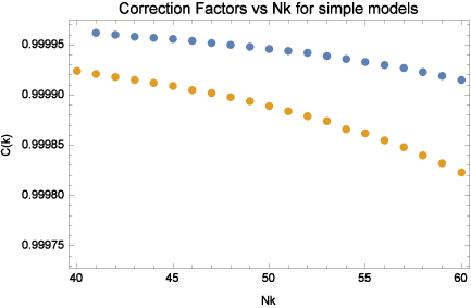
Figure 5 also answers the first of the questions posed at the end of the Introduction: it seems that the constant $\epsilon$ approximation is most accurate for $\epsilon$ near to $\epsilon_{k}$ . One can see this by comparing the value of the correction factor $C(\epsilon)$ , defined in (26), with the nonlocal correction factor $\mathcal{C}(k)$ shown in Figure 5, over the 20 e-foldings of first horizon crossing ( $40<N_{k}<60$ ) depicted,

	$\displaystyle V(\varphi)\propto\varphi^{2}$	$\displaystyle\Longrightarrow$	$\displaystyle\Biggl\{{0.99546<C(\epsilon_{k})<0.99317\atop 0.99996<\mathcal{C}(k)<0.99991}\Biggr\}\;,$		(100)
	$\displaystyle V(\varphi)\propto\varphi^{4}$	$\displaystyle\Longrightarrow$	$\displaystyle\Biggl\{{0.99084<C(\epsilon_{k})<0.98619\atop 0.99992<\mathcal{C}(k)<0.99982}\Biggr\}\;.$		(101)

There is about 50 times more variation in $C(\epsilon_{k})$ than in $\mathcal{C}(k)$ , limiting the potential improvement to a positive offset of about $\Delta N\approx\frac{20}{50}=0.4$ . Because other models show $\mathcal{C}(k)>1$ there is actually no preference for shifting the point at which $\epsilon$ is evaluated.

5.2 $\mathcal{C}(k)\!-\!1$ significant for changes near horizon crossing

It has also long been understood that the constant $\epsilon$ formulae require significant corrections when $\epsilon(N)$ suffers large variation within several e-foldings of first horizon crossing [66, 67]. We already saw this in the exact results depricted in Figure 2 for an instantaneous jump in $\epsilon$ . Figure 6 makes the same point for two smooth transitions. The left hand graph shows the effect on $\mathcal{C}(k)$ of a smooth transition from $\epsilon=0$ to $\epsilon=\frac{1}{2}$ via a logistic function centered at a critical value $N_{c}$ ,

\epsilon(N)=\frac{0.5}{1+e^{N_{c}-N}}\;.

(102)

The right hand graph shows $\mathcal{C}(k)$ for a $V(\varphi)\propto\varphi^{2}$ model which experiences a Gaussian bump, centered at $N_{c}$ , which actually induces a brief deceleration,

\epsilon(N)=\frac{1}{200\!-\!2N}+\exp\Bigl[-10(N\!-\!N_{c})^{2}\Bigr]\;.

(103)

This is one of the models for which $\mathcal{C}(k)$ is larger than one.

5.3 Eqn. (96) is quite accurate near horizon crossing

The previous two points were known before in general terms. Our contributions in this paper are:

1.

An analytic quantification — through the asymptotic expansions (84) and (89) — of when to expect significant corrections to the constant $\epsilon$ approximation; and
2.

An analytic approximation (96) of the function $h(t,k)$ which gives us the nonlocal correction factor through expression (97).

Figure 7 show just how accurate our approximation is in the period before first horizon crossing. It even catches the turning points at $N\sim 49.8$ .

Our analytic approximation (96) continues to be very accurate after first horizon crossing for models in which there is no significant evolution of $\epsilon(t)$ at late times. Figure 8 illustrates this by showing $h(t,k)$ versus $N$ for a class of models in which $\epsilon$ makes a transition (centered about horizon crossing of $N_{k}=50$ ) from an early value of $\epsilon=\frac{1}{200}$ to a late value of $\epsilon=\frac{1}{10}$ through a logistic function with steepness parameter $K=1,2,10$ ,

\epsilon(N)=\frac{1}{200}+\frac{\frac{19}{200}}{1\!+\!\exp[-K(N\!-\!N_{k})]}\;.

(104)

In each case the horizon crossing value is $\epsilon_{k}=\frac{41}{400}$ .

Note from Figure 8 that the final value of $h(t,k)$ is largest when the transition is most gradual. Because the full amplitude is $M(t,k)=M_{0}(t,k)\!\times\!\exp[-\frac{1}{2}h(t,k)]$ , one might expect that $M(t,k)$ therefore freezes in to a smaller amplitude for a more gradual transition. In fact the reverse is true because only the value of $\epsilon$ near horizon crossing is relevant, so making $\epsilon$ stay small longer causes the freeze-in amplitude to be larger. This is evident from the nonlocal correction factors $\mathcal{C}(k)$ for the three cases,

$\displaystyle K=1$	$\displaystyle\Longrightarrow$	$\displaystyle\mathcal{C}(k)=0.993556\qquad(0.994121)\;,$	(105)
$\displaystyle K=2$	$\displaystyle\Longrightarrow$	$\displaystyle\mathcal{C}(k)=0.989201\qquad(0.989418)\;,$	(106)
$\displaystyle K=10$	$\displaystyle\Longrightarrow$	$\displaystyle\mathcal{C}(k)=0.975152\qquad(0.975230)\;.$	(107)

(The parenthesized values are for the linearized approximation, which shows that it is indeed quite good.) We fixed the values of $H(t_{k})$ and $a(t_{k})$ to be the same for each model, so these correction factors give the relative freeze-in amplitudes for $M(t,k)$ .

The much larger and opposite-sense effect which is evident in the asymptotic values of $h(t,k)$ of Figure 8 is needed to compensate for the factor $M_{0}(t,k)$ . Recall from section 3.2 that if $\epsilon(t)$ becomes constant at $\epsilon_{1}$ for times $t>t_{1}$ then we can write,

\epsilon(t)=\epsilon_{1}\qquad\Longrightarrow\qquad H(t)a^{\epsilon_{1}}(t)=H_{1}a_{1}^{\epsilon_{1}}\;,

(108)

where $H_{1}\equiv H(t_{1})$ and $a_{1}\equiv a(t_{1})$ . Each of the three models has effectively reached this condition by 10 e-foldings after first horizon crossing, but the values of $H_{1}$ and $a_{1}$ are smaller the steeper the transition. That affects the factor of $M_{0}(t,k)$ , which approaches a constant given by (22),

M_{0}(t,k)\longrightarrow\frac{H^{2}(t_{k})}{2k^{3}}\!\times\!C(\epsilon_{1})\!\times\!\Biggl[\frac{H_{1}a_{1}^{\epsilon_{1}}}{H(t_{k})a^{\epsilon_{1}}(t_{k})}\Biggr]^{\frac{2}{1-\epsilon_{1}}}\;.

(109)

The final factor of (109) is significantly larger for more gradual transitions, which is mostly cancelled by the larger asymptotic values of $h(t,k)$ , to leave the small effect evident in the nonlocal correction factors (105-107).

The same late time effect of $h(t,k)$ partially compensating for changes in $M_{0}(t,k)$ is evident from the results for $V(\varphi)\propto\varphi^{2}$ and $V(\varphi)\propto\varphi^{4}$ models displayed in Figure 9. In this case $\epsilon(t)$ continues to evolve after first horizon crossing. Considered as a function of $N$ we have $\partial_{N}\ln[H(N)]=-\epsilon(N)$ , so the asymptotic form (89) can be re-expressed as,

h(t,k)=\frac{4}{1\!-\!\epsilon(N)}\!\int_{N_{k}}^{N}\!\!\!\!\!dn\Delta n\epsilon^{\prime}(n)+2\ln\Bigl[\frac{C(\epsilon(N))}{C(\epsilon_{k})}\Bigr]-2\ln\Bigl[\mathcal{C}(k)\Bigr]+O\Bigl(e^{-2\Delta N}\Bigr)\;,

(110)

where $\Delta n\equiv n-N_{k}$ and $\Delta N\equiv N-N_{k}$ . Because $\epsilon$ typically grows slowly with $N$ (as it does for both of the models in Figure 9) the integral grows and dominates the slowly falling logarithm of (110), so that $h(t,k)$ grows like $\Delta N^{2}$ . This growth is evident for both models in Figure 9.

5.4 Problems long after horizon crossing

Of course too much growth endangers the linearized approximation we made in passing from the full equation (75) to (90). Recall that this entails changing two terms,

	$\displaystyle-\Bigl[\frac{1}{2}\partial_{N}h\Bigr]^{2}$	$\displaystyle\longrightarrow$	$\displaystyle 0\;,$		(111)
	$\displaystyle\exp\Bigl[h(t,k)\Bigr]\!-\!1$	$\displaystyle\longrightarrow$	$\displaystyle h(t,k)\;.$		(112)

There is never any problem with (112) because $h(t,k)$ is small before first horizon crossing and the coefficient of this term is minuscule after first horizon crossing. The problematic approximation is (111), although only in the region after first horizon crossing for models in which $\epsilon$ evolves at very late times. One can see from expression (87) that two terms contribute to provide the factor of $F^{2}\sim\Delta N^{2}$ (recall the definition (86) of $F$ ) which is evident in the late time evolution equation (85),

	$\displaystyle-\Bigl[\frac{1}{2}\partial_{N}h\Bigr]^{2}$	$\displaystyle\longrightarrow$	$\displaystyle-\Bigl[2\partial_{N}\epsilon\,\Delta\nu^{2}F\Bigr]^{2}\;,$		(113)
	$\displaystyle 2\partial_{N}\epsilon\,\Delta\nu^{2}F\!\times\!\partial_{N}h$	$\displaystyle\longrightarrow$	$\displaystyle+2\Bigl[2\partial_{N}\epsilon\,\Delta\nu^{2}F\Bigr]^{2}\;.$		(114)

These terms are enhanced by the factor of $F^{2}\sim\Delta N^{2}$ but suppressed by $(\partial_{N}\epsilon)^{2}$ . In the full nonlinear equation (113) cancels half of (114), but this cancellation does not happen in the linearized equation because (113) is not present. Hence we expect the very late time growth of the linearized approximation (96) to be less than what it is for the actual solution. This is barely evident in Figure 10 for the $V(\varphi)\propto\varphi^{2}$ model at very late times.

The problem we have just described might seem serious but it is not. The full amplitude $M(t,k)=M_{0}(t,k)\times\exp[-\frac{1}{2}h(t,k)]$ really does become constant shortly after first horizon crossing. The growth of $h(t,k)$ is only an artifact of the our having factored out by $M_{0}(t,k)$ , which also grows for models in which $\epsilon$ increases at late times. Because the problem has such a simple origin, there are two easy fixes:

1.

Either evaluate $\mathcal{C}(k)$ using expression (97) at some point $N_{2}$ before nonlinear effects become important; or
2.

Subtract the right hand side of (113) from the source $\mathcal{S}(N,N_{k})$ in the Green’s function solution.

6 Epilogue

The full scalar and tensor power spectra can be expressed in terms of two amplitudes $N(t,k)$ and $M(t,k)$ ,

	$\displaystyle\Delta^{2}_{\mathcal{R}}(k)$	$\displaystyle=$	$\displaystyle\frac{2Gk^{3}}{\pi}\!\times\!N\Bigl(t\!\gg\!t_{k},k\Bigr)\!\times\!\Biggl\{1+O(GH^{2})\Biggr\}\;,$		(115)
	$\displaystyle\Delta^{2}_{h}(k)$	$\displaystyle=$	$\displaystyle\frac{32Gk^{3}}{\pi}\!\times\!M\Bigl(t\!\gg\!t_{k},k\Bigr)\!\times\!\Biggl\{1+O(GH^{2})\Biggr\}\;.$		(116)

If the one loop corrections of order $GH^{2}\mathrel{\raise 1.29167pt\hbox{$<$\kern-7.5pt\lower 4.30554pt\hbox{$\sim$}}}10^{-11}$ are ever to resolved we must have precise predictions for the two amplitudes. Part of this problem entails finding a unique model for primordial inflation, which is beyond the scope of our present effort. We have instead focussed on predicting how the amplitudes depend upon the inflationary expansion history $a(t)$ . Our analysis is based on earlier work in which nonlinear equations for the two amplitudes were derived [44, 45].

Because the transformation (17) carries $M(t,k)$ into $N(t,k)$ , we worked with the simpler tensor amplitude. We express its late time limiting form as,

M\Bigl(t\gg t_{k},k\Bigr)=\frac{H^{2}(t_{k})}{2k^{3}}\!\times\!C\Bigl(\epsilon(t_{k})\Bigr)\!\times\!\mathcal{C}(k)\;,

(117)

where $C(\epsilon)$ was defined in expression (26) and graphed in Figure 1. Our numerical studies show that this factor really does need to present, and it is best to evaluate it at the time $t_{k}$ of first horizon crossing. The remaining factor $\mathcal{C}(k)$ represents nonlocal effects from the expansion history before and after first horizon crossing. It has long been clear that this factor is close to unity for models in which $\epsilon(t)$ is smooth near first horizon crossing, but $\mathcal{C}(k)$ can give significant corrections when there are large changes within a few e-foldings of first horizon crossing [66, 67].

Our key results (89) and (97) give, for the first time ever, a good analytic approximation for the nonlocal correction factor $\mathcal{C}(k)$ . Our technique was to first get close to the exact solution by factoring out the known, constant $\epsilon$ solution $M_{0}(t,k)$ ,

M(t,k)=M_{0}(t,k)\!\times\!\exp\Bigl[-\frac{1}{2}h(t,k)\Bigr]\;.

(118)

Of course this means that the evolution equation (75) for $h(t,k)$ is driven by a source term which vanishes whenever $\epsilon(t)$ is constant. From the equation’s asymptotic early time form (79) we can see that that $h(t,k)$ behaves as a damped, driven harmonic oscillator. For more than a few e-foldings before first horizon crossing the restoring force (81) is so large that $h(t,k)$ is both small and completely determined by local conditions according to a wonderfully convergent expansion (84). That is evident from Figure 2 even for an instantaneous jump in $\epsilon(t)$ .

As long as $\partial_{N}h(t,k)$ remains small the full equation (75) can be linearized to a form (90) for which we were able to derive a Green’s function solution (96). It cannot be overstressed that this solution pertains for an arbitrary inflationary expansion history. The assumption of linearity on which it is based should be valid long before first horizon crossing. It can break down long after first horizon crossing but in a way which is very simple to repair.

Our formalism differs from the generalized slow roll approximation [46, 47] in three ways:

1.

Instead of correcting the mode function $u(t,k)$ and then inferring how this affects $M(t,k)\equiv|u(t,k)|^{2}$ , we correct $M(t,k)$ directly;
2.

Our 0th order term is exact for arbitrary constant $\epsilon(t)$ ; and
3.

Our corrections are multiplicative rather than additive.

As the early time expansions (64) and (60) show, our formalism captures effects at first order which require going to second order in the generalized slow roll expansion. Given a specific model, the additional accuracy of our formalism is not required for the analysis of current data. Its advantage derives rather from the more explicit connection it makes between data and a general, initially unknown model. This has potential applications for the power spectra on three time scales:

1.

For current data it facilitates the process of inferring the sorts of models which might explain anomalies;
2.

For next generation data, which might begin resolving the tensor power spectrum, it permits exploitation of the general relation (17) between the tensor and scalar power spectra to develop a version of the single scalar consistency relation [48, 49, 50] that could be employed before the tensor spectral index has been well measured; and
3.

For far future data, when the full development of 21 cm cosmology might permit loop corrections to be resolved, it elucidates both when the loop counting parameter of $GH^{2}(t)$ should be evaluated, and whether or not there can be enhancements of the form $\epsilon_{\rm late}/\epsilon_{\rm early}$ .

Our work also has three more general applications. First, there is a close relation between $M(t,k)$ and the vacuum expectation value of a massless, minimally coupled (MMC) scalar,

\Bigl\langle\Omega\Bigl|\varphi^{2}(t,\vec{x})\Bigr|\Omega\Bigr\rangle=\int\!\!\frac{dkk^{2}}{2\pi^{2}}\,M(t,k)\;.

(119)

This relation should allow us to estimate the secular growth for an arbitrary inflationary expansion history, which is an important step in building nonlocal models to represent the quantum gravitational back-reaction on inflation [52, 53, 54, 71]. Second, note that our transformation (17) could be used to convert the propagator of a MMC scalar into the propagator for the scalar perturbation field $\zeta(t,\vec{x})$ for an arbitrary inflationary expansion history. Of course we do not have MMC scalar propagator for arbitrary $a(t)$ but perhaps the transformation could be used to derive relations between loops involving gravitons and loops involving $\zeta$ . Finally, our technique for passing from the oscillatory mode functions to their norm-squared [44, 45] can be applied for any perturbations whose mode functions obey second order equations. It would be interesting to see what it gives for Higgs inflation and for $f(R)$ models of inflation.

Acknowledgements

We are grateful for conversations and correspondence on this subject with P. K. S. Dunsby, S. Odintsov, L. Patino, M. Romania, S. Shandera and M. Sloth. This work was partially supported by the European Union (European Social Fund, ESF) and Hellenic national funds through the Operational Program “Education and Lifelong Learning” of the National Strategic Reference Framework (NSRF) under the “ $\Theta\alpha\lambda\acute{\eta}\varsigma$ ” action MIS-375734, under the “ $A\rho\iota\sigma\tau\epsilon\acute{\iota}\alpha$ ” action, under the “Funding of proposals that have received a positive evaluation in the 3rd and 4th Call of ERC Grant Schemes”; by NSF grants PHY-1205591 and PHY-1506513, and by the Institute for Fundamental Theory at the University of Florida.

7 Appendix A: Simplifying Equation (72)

The first time derivative of $M_{0}(t,k)$ is,

\dot{M}_{0}=-2HM_{0}+\dot{z}M_{0}^{\prime}+\dot{\nu}\partial_{\nu}M_{0}\;.

(120)

where a prime stands for the derivative with respect to $z$ and $\partial_{\nu}$ denotes differentiation with respect to $\nu$ . It is best to postpone using the explicit expressions for $\dot{z}$ and $\dot{\nu}$ ,

\dot{z}=-\frac{k}{a}+\frac{\dot{\epsilon}}{1\!-\!\epsilon}\times z\qquad,\qquad\dot{\nu}=\frac{\dot{\epsilon}}{(1\!-\!\epsilon)^{2}}\;.

(121)

The time second derivative of $M_{0}(t,k)$ is,

	$\displaystyle\ddot{M}_{0}=\Bigl(4\!+\!2\epsilon\Bigr)H^{2}M_{0}+\Bigl(-4H\dot{z}\!+\!\ddot{z}\Bigr)M_{0}^{\prime}+\Bigl(-4H\dot{\nu}\!+\!\ddot{\nu}\Bigr)\partial_{\nu}M_{0}$				(122)
			$\displaystyle\hskip 170.71652pt+\dot{z}^{2}M_{0}^{\prime\prime}+2\dot{z}\dot{\nu}\partial_{\nu}M_{0}^{\prime}+\dot{\nu}^{2}\partial_{\nu}^{2}M_{0}\;.\qquad$		(122)

Bessel’s equation implies that $M_{0}^{\prime\prime}$ can be eliminated using,

M_{0}^{\prime\prime}+2M_{0}-2(2\!-\!\epsilon)\frac{H^{2}a^{2}}{k^{2}}M_{0}=\frac{1}{2M_{0}}\Bigl[{M_{0}^{\prime}}^{2}+\frac{1}{k^{2}a^{4}}\Bigr]\;.

(123)

The other derivatives we require are,

	$\displaystyle 3H\dot{M}_{0}$	$\displaystyle=$	$\displaystyle-6H^{2}M_{0}+3H\dot{z}M_{0}^{\prime}+3H\dot{\nu}\partial_{\nu}M_{0}\;,\qquad$		(124)
	$\displaystyle-\frac{\dot{M}_{0}^{2}}{2M_{0}}$	$\displaystyle=$	$\displaystyle-2H^{2}M_{0}+2H\dot{z}M_{0}^{\prime}+2H\dot{\nu}\partial_{\nu}M_{0}-\frac{(\dot{z}M_{0}^{\prime}\!+\!\dot{\nu}\partial_{\nu}M_{0})^{2}}{2M_{0}}\;.\qquad$		(125)

Substituting everything into the definition (72) of $S(t,k)$ gives,

	$\displaystyle S(t,k)=-(H\dot{z}\!+\!\ddot{z})\frac{M_{0}^{\prime}}{M_{0}}-(H\dot{\nu}\!+\!\ddot{\nu})\frac{\partial_{\nu}M_{0}}{M_{0}}-2\dot{z}\dot{\nu}\Bigl[\frac{\partial_{\nu}M_{0}^{\prime}}{M_{0}}\!-\!\frac{M_{0}^{\prime}}{2M_{0}}\frac{\partial_{\nu}M_{0}}{M_{0}}\Bigr]$				(126)
			$\displaystyle\hskip 0.0pt-\dot{\nu}^{2}\Bigl[\frac{\partial_{\nu}^{2}M_{0}}{M_{0}}\!-\!\frac{1}{2}\Bigl(\frac{\partial_{\nu}M_{0}}{M_{0}}\Bigr)^{2}\Bigr]-\Bigl(\dot{z}^{2}\!-\!\frac{k^{2}}{a^{2}}\Bigr)\Biggl\{\frac{(4\!-\!2\epsilon)}{(1\!-\!\epsilon)^{2}z^{2}}-2+\frac{1}{2k^{2}a^{4}M_{0}^{2}}\Biggr\}.\qquad$		(126)

Each of the five terms on the right hand side of (126) is proportional to at least one derivative of $\epsilon(t)$ . Before exhibiting this it is desirable to isolate the $\epsilon$ -dependent part of the index $\nu$ , and to change from co-moving time $t$ to the number of e-foldings since the beginning of inflation $N\equiv\ln[a(t)/a_{i}]$ ,

\Delta\nu\equiv\frac{1}{1\!-\!\epsilon}\qquad,\qquad\frac{d}{dt}=H\frac{d}{dN}\quad,\quad\frac{d^{2}}{dt^{2}}=H^{2}\Bigl[\frac{d^{2}}{dN^{2}}\!-\!\epsilon\frac{d}{dN}\Bigr]\;.

(127)

With this notation the five prefactors from the right hand side of (126) are,

$\displaystyle H\dot{z}\!+\!\ddot{z}$	$\displaystyle\!\!\!\!\!=\!\!\!\!\!$	$\displaystyle\Bigl[\frac{H\epsilon\dot{\epsilon}}{1\!-\!\epsilon}\!+\!\frac{\ddot{\epsilon}}{1\!-\!\epsilon}\!+\!2\Bigl(\frac{\dot{\epsilon}}{1\!-\!\epsilon}\Bigr)^{2}\Bigr]z=H^{2}\Bigl[\frac{\partial_{N}^{2}\epsilon}{1\!-\!\epsilon}\!+\!2\Bigl(\frac{\partial_{N}\epsilon}{1\!-\!\epsilon}\Bigr)^{2}\Bigr]z\;,\qquad$	(128)
$\displaystyle H\dot{\nu}\!+\!\ddot{\nu}$	$\displaystyle\!\!\!\!\!=\!\!\!\!\!$	$\displaystyle\Bigl[\frac{H\dot{\epsilon}}{1\!-\!\epsilon}\!+\!\frac{\ddot{\epsilon}}{1\!-\!\epsilon}\!+\!2\Bigl(\frac{\dot{\epsilon}}{1\!-\!\epsilon}\Bigr)^{2}\Bigr]\Delta\nu\!=\!H^{2}\Bigl[\partial_{N}\epsilon\!+\!\frac{\partial_{N}^{2}\epsilon}{1\!-\!\epsilon}\!+\!2\Bigl(\frac{\partial_{N}\epsilon}{1\!-\!\epsilon}\Bigr)^{2}\Bigr]\Delta\nu\;,\quad$	(129)
$\displaystyle 2\dot{z}\dot{\nu}$	$\displaystyle\!\!\!\!\!=\!\!\!\!\!$	$\displaystyle\Bigl[-2H\dot{\epsilon}+2\Bigl(\frac{\dot{\epsilon}}{1\!-\!\epsilon}\Bigr)^{2}\Bigr]z\Delta\nu=H^{2}\Bigl[-2\partial_{N}\epsilon\!+\!2\Bigl(\frac{\partial_{N}\epsilon}{1\!-\!\epsilon}\Bigr)^{2}\Bigr]z\Delta\nu\;,$	(130)
$\displaystyle\dot{\nu}^{2}$	$\displaystyle\!\!\!\!\!=\!\!\!\!\!$	$\displaystyle\Bigl(\frac{\dot{\epsilon}}{1\!-\!\epsilon}\Bigr)^{2}\Delta\nu^{2}=H^{2}\Bigl(\frac{\partial_{N}\epsilon}{1\!-\!\epsilon}\Bigr)^{2}\Delta\nu^{2}\;,$	(131)
$\displaystyle\dot{z}^{2}\!-\!\frac{k^{2}}{a^{2}}$	$\displaystyle\!\!\!\!\!=\!\!\!\!\!$	$\displaystyle\Bigl[-2H\dot{\epsilon}\!+\!\Bigl(\frac{\dot{\epsilon}}{1\!-\!\epsilon}\Bigr)^{2}\Bigr]z^{2}=H^{2}\Bigl[-2\partial_{N}\epsilon\!+\!\Bigl(\frac{\partial_{N}\epsilon}{1\!-\!\epsilon}\Bigr)^{2}\Bigr]z^{2}\;.$	(132)

In comparing expressions (128-132) with (126) it will be seen that every derivative with respect to $z$ is paired with one factor of $z$ , and every derivative with respect to $\nu$ is paired with one factor of $\Delta\nu$ . This suggests differentiating with respect to the logarithms,

\zeta\equiv\ln(z)\quad\Longrightarrow\quad z\frac{\partial}{\partial z}=\frac{\partial}{\partial\zeta}\quad,\quad\xi\equiv\ln(\Delta\nu)\quad\Longrightarrow\quad\Delta\nu\frac{\partial}{\partial\nu}=\frac{\partial}{\partial\xi}\;.

(133)

From (126) it is also apparent that the factor of $2ka^{2}$ in the denominator of $M_{0}(t,k)$ is always cancelled, either by ratios or explicit factors. It is best to define a new variable for the logarithm of the factor in the numerator (74),

\sigma(z,\nu)\equiv\ln\Biggl[\frac{\pi z}{2}\Bigl|H^{(1)}_{\nu}(z)\Bigr|^{2}\Biggr]=\ln\Biggl[\frac{\pi z}{2}\Bigl[J_{\nu}^{2}(z)\!+\!N_{\nu}^{2}(z)\Bigr]\Biggr]\;.

(134)

Our final form for the source is therefore,

$\displaystyle\frac{S(t,k)}{H^{2}}=-\Bigl[\frac{\partial_{N}^{2}\epsilon}{1\!-\!\epsilon}\!+\!2\Bigl(\frac{\partial_{N}\epsilon}{1\!-\!\epsilon}\Bigr)^{2}\Bigr]\frac{\partial\sigma}{\partial\zeta}-\Bigl[\partial_{N}\epsilon\!+\!\frac{\partial_{N}^{2}\epsilon}{1\!-\!\epsilon}\!+\!2\Bigl(\frac{\partial_{N}\epsilon}{1\!-\!\epsilon}\Bigr)^{2}\Bigr]\frac{\partial\sigma}{\partial\xi}$		(135)
	$\displaystyle\hskip-8.5359pt-2\Bigl[-\partial_{N}\epsilon\!+\!\Bigl(\frac{\partial_{N}\epsilon}{1\!-\!\epsilon}\Bigr)^{2}\Bigr]\Bigl[\frac{\partial^{2}\sigma}{\partial\zeta\partial\xi}\!+\!\frac{1}{2}\frac{\partial\sigma}{\partial\zeta}\frac{\partial\sigma}{\partial\xi}\Bigr]-\Bigl(\frac{\partial_{N}\epsilon}{1\!-\!\epsilon}\Bigr)^{2}\Bigl[\frac{\partial^{2}\sigma}{\partial\xi^{2}}\!-\!\frac{\partial\sigma}{\partial\xi}\!+\!\frac{1}{2}\Bigl(\frac{\partial\sigma}{\partial\xi}\Bigr)^{2}\Bigr]$
	$\displaystyle\hskip 99.58464pt-2\Bigl[-2\partial_{N}\epsilon\!+\!\Bigl(\frac{\partial_{N}\epsilon}{1\!-\!\epsilon}\Bigr)^{2}\Bigr]\Bigl[\frac{(2\!-\!\epsilon)}{(1\!-\!\epsilon)^{2}}+e^{2\zeta}(e^{-2\sigma}\!-\!1)\Bigr]\;.$

We obviously want to make the same changes on the left hand side of (126). It is also desirable to change the dependent variable from $\Delta M$ to $h(t,k)\equiv-2\ln[\Delta M(t,k)]$ , all of which implies,

	$\displaystyle\frac{\Delta\ddot{M}}{\Delta M}+\Bigl[3H+\frac{\dot{M}_{0}}{M_{0}}\Bigr]\frac{\Delta\dot{M}}{\Delta M}-\frac{1}{2}\Bigl(\frac{\Delta\dot{M}}{\Delta M}\Bigr)^{2}+\frac{1}{2a^{6}M_{0}^{2}}\Bigl[1\!-\!\frac{1}{\Delta M^{2}}\Bigr]\Biggr]$				(136)
			$\displaystyle\hskip-14.22636pt=-\frac{H^{2}}{2}\Biggl\{\partial^{2}_{N}h\!-\!\Bigl[\frac{1}{2}\partial_{N}h\Bigr]^{2}\!+\!\Bigl[1\!-\!\epsilon\!+\!\partial_{N}\sigma\Bigr]\partial_{N}h\!+\!\Bigl[2(1\!-\!\epsilon)e^{\zeta-\sigma}\Bigr]^{2}\Bigl[e^{h}\!-\!1\Bigr]\Biggr\}.\qquad$		(136)

Equating (135) to (136) and dividing out the common factor of $-\frac{1}{2}H^{2}$ gives the final form (75) of our evolution equation.

8 Appendix B: Equation (75) at Early Times

In the early time regime the parameter $z(t,k)\equiv\frac{k}{(1-\epsilon)Ha}$ is large which implies,

\frac{\pi z}{2}\Bigl|H^{(1)}_{\nu}(z)\Bigr|^{2}=1+\frac{(\nu^{2}\!-\!\frac{1}{4})}{2z^{2}}+\frac{3(\nu^{2}\!-\!\frac{1}{4})(\nu^{2}\!-\!\frac{9}{4})}{8z^{4}}+O\Bigl(\frac{1}{z^{6}}\Bigr)\;.

(137)

Hence the early time expansion for $\sigma(z,\nu)$ is,

\sigma(z,\nu)=\frac{(\nu^{2}\!-\!\frac{1}{4})}{2z^{2}}+\frac{(\nu^{2}\!-\!\frac{1}{4})(\nu^{2}\!-\!\frac{13}{4})}{4z^{4}}+\dots

(138)

Expression (138) implies the following expansions for the various $\sigma$ -dependent factors in (75),

$\displaystyle\Bigl[1\!-\!\epsilon\!+\!\partial_{N}\sigma\Bigr]$	$\displaystyle=$	$\displaystyle 1\!-\!\epsilon+O\Bigl(\frac{1}{z^{2}}\Bigr)\;,$	(139)
$\displaystyle\Bigl[2(1\!-\!\epsilon)e^{\zeta-\sigma}\Bigr]^{2}$	$\displaystyle=$	$\displaystyle 4(1\!-\!\epsilon)^{2}z^{2}+O(1)\;,$	(140)
$\displaystyle\frac{\partial\sigma}{\partial\zeta}=-\frac{(\nu^{2}\!-\!\frac{1}{4})}{z^{2}}+O\Bigl(\frac{1}{z^{4}}\Bigr)$	,	$\displaystyle\frac{\partial\sigma}{\partial\xi}=\frac{(\nu^{2}\!-\!\frac{1}{2}\nu)}{z^{2}}+O\Bigl(\frac{1}{z^{4}}\Bigr)\;,$	(141)
$\displaystyle\Bigl[\frac{\partial^{2}\sigma}{\partial\zeta\partial\xi}\!+\!\frac{1}{2}\frac{\partial\sigma}{\partial\zeta}\frac{\partial\sigma}{\partial\xi}\Bigr]$	$\displaystyle=$	$\displaystyle-\frac{(2\nu^{2}\!-\!\nu)}{z^{2}}+O\Bigl(\frac{1}{z^{4}}\Bigr)\;,$	(142)
$\displaystyle\Bigl[\frac{\partial^{2}\sigma}{\partial\xi^{2}}\!-\!\frac{\partial\sigma}{\partial\xi}\!+\!\frac{1}{2}\Bigl(\frac{\partial\sigma}{\partial\xi}\Bigr)^{2}\Bigr]$	$\displaystyle=$	$\displaystyle\frac{(\nu\!-\!\frac{1}{2})^{2}}{z^{2}}+O\Bigl(\frac{1}{z^{4}}\Bigr)\;,$	(143)
$\displaystyle\Bigl[\frac{(2\!-\!\epsilon)}{(1\!-\!\epsilon)^{2}}+e^{2\zeta}(e^{-2\sigma}\!-\!1)\Bigr]$	$\displaystyle=$	$\displaystyle\frac{3(\nu^{2}\!-\!\frac{1}{4})}{2z^{2}}+O\Bigl(\frac{1}{z^{4}}\Bigr)\;.$	(144)

Substituting these expansions in (75) and additionally neglecting nonlinear terms in $h(t,k)$ gives equation (79).

9 Appendix C: Equation (75) at Late Times

In the late time regime of $z(t,k)\ll 1$ , but still with $0\leq\epsilon(t)<1$ , it is the small argument expansion of the Neumann function in (134) which controls the behavior of $\sigma(z,\nu)$ ,

\sigma=\ln\Biggl[\frac{\Gamma^{2}(\nu)}{\pi}\Bigl(\frac{2}{z}\Bigr)^{2\nu-1}\Biggr]+O(z^{2})=2\Delta\nu\Biggl[\Delta N\!+\!\ln\Bigl[\frac{H}{H(t_{k})}\Bigr]\Biggr]+\ln\Bigl[C(\epsilon)\Bigr]+O(z^{2})\;.

(145)

Its derivative involves the digamma function $\psi(z)\equiv\frac{d}{dz}\ln[\Gamma(z)]$ ,

\partial_{N}\sigma=2+2\Delta\nu\frac{\partial_{N}\epsilon}{1\!-\!\epsilon}\Bigl[-1\!-\!\ln\Bigl(\frac{z}{2}\Bigr)\!+\!\psi\Bigl(\frac{1}{2}\!+\!\Delta\nu\Bigr)\Bigr]+O(z^{2})\;.

(146)

The term in square brackets is defined in expression (86) and grows roughly linearly in $N$ . The seven $\sigma$ -dependent factors of expression (75) have the expansions,

$\displaystyle\Bigl[1\!-\!\epsilon\!+\!\partial_{N}\sigma\Bigr]$	$\displaystyle=$	$\displaystyle 3\!-\!\epsilon+\frac{\partial_{N}\epsilon}{1\!-\!\epsilon}\times 2\Delta\nu F+O(z^{2})\;,$	(147)
$\displaystyle\Bigl[2(1\!-\!\epsilon)e^{\zeta-\sigma}\Bigr]^{2}$	$\displaystyle=$	$\displaystyle 4(1\!-\!\epsilon)^{2}z^{2}\times\Bigl(\frac{z}{2}\Bigr)^{4\Delta\nu}\frac{\pi^{2}}{\Gamma^{4}(\nu)}+O(z^{4+4\Delta\nu})\;,\qquad$	(148)
$\displaystyle\frac{\partial\sigma}{\partial\zeta}=-2\Delta\nu+O(z^{2})$	,	$\displaystyle\frac{\partial\sigma}{\partial\xi}=2\Delta\nu(F\!+\!1)+O(z^{2})\;,$	(149)
$\displaystyle\Bigl[\frac{\partial^{2}\sigma}{\partial\zeta\partial\xi}\!+\!\frac{1}{2}\frac{\partial\sigma}{\partial\zeta}\frac{\partial\sigma}{\partial\xi}\Bigr]$	$\displaystyle=$	$\displaystyle-2\Delta\nu^{2}(F\!+\!1)-2\Delta\nu+O(z^{2})\;,$	(150)
$\displaystyle\Bigl[\frac{\partial^{2}\sigma}{\partial\xi^{2}}\!-\!\frac{\partial\sigma}{\partial\xi}\!+\!\frac{1}{2}\Bigl(\frac{\partial\sigma}{\partial\xi}\Bigr)^{2}\Bigr]$	$\displaystyle=$	$\displaystyle 2\Delta\nu^{2}\Bigl[(F\!+\!1)^{2}+\psi^{\prime}\Bigl(\frac{1}{2}\!+\!\Delta\nu\Bigr)\Bigr]+O(z^{2})\;,$	(151)
$\displaystyle\Bigl[\frac{(2\!-\!\epsilon)}{(1\!-\!\epsilon)^{2}}+e^{2\zeta}(e^{-2\sigma}\!-\!1)\Bigr]$	$\displaystyle=$	$\displaystyle\Delta\nu+\Delta\nu^{2}+O(z^{2})\;.$	(152)

From (148) the restoring force drops out of (75) but all the other terms contribute to give the late time limiting form (85).

References

[1] A. A. Starobinsky, JETP Lett. 30, 682 (1979) [Pisma Zh. Eksp. Teor. Fiz. 30, 719 (1979)].
[2] V. F. Mukhanov and G. V. Chibisov, JETP Lett. 33, 532 (1981) [Pisma Zh. Eksp. Teor. Fiz. 33, 549 (1981)].
[3] R. P. Woodard, Rept. Prog. Phys. 72, 126002 (2009) [arXiv:0907.4238 [gr-qc]].
[4] A. Ashoorioon, P. S. Bhupal Dev and A. Mazumdar, Mod. Phys. Lett. A 29, no. 30, 1450163 (2014) [arXiv:1211.4678 [hep-th]].
[5] L. M. Krauss and F. Wilczek, Phys. Rev. D 89, no. 4, 047501 (2014) [arXiv:1309.5343 [hep-th]].
[6] G. F. Smoot, C. L. Bennett, A. Kogut, E. L. Wright, J. Aymon, N. W. Boggess, E. S. Cheng and G. De Amici et al., Astrophys. J. 396, L1 (1992).
[7] G. Hinshaw et al. [WMAP Collaboration], Astrophys. J. Suppl. 208, 19 (2013) [arXiv:1212.5226 [astro-ph.CO]].
[8] Z. Hou, C. L. Reichardt, K. T. Story, B. Follin, R. Keisler, K. A. Aird, B. A. Benson and L. E. Bleem et al., Astrophys. J. 782, 74 (2014) [arXiv:1212.6267 [astro-ph.CO]].
[9] J. L. Sievers et al. [Atacama Cosmology Telescope Collaboration], JCAP 1310, 060 (2013) [arXiv:1301.0824 [astro-ph.CO]].
[10] P. A. R. Ade et al. [Planck Collaboration], Astron. Astrophys. 571, A16 (2014) [arXiv:1303.5076 [astro-ph.CO]].
[11] P. A. R. Ade et al. [BICEP2 Collaboration], Phys. Rev. Lett. 112, no. 24, 241101 (2014) [arXiv:1403.3985 [astro-ph.CO]].
[12] R. Adam et al. [Planck Collaboration], arXiv:1409.5738 [astro-ph.CO].
[13] P. A. R. Ade et al. [BICEP2 and Planck Collaborations], Phys. Rev. Lett. 114, no. 10, 101301 (2015) [arXiv:1502.00612 [astro-ph.CO]].
[14] P. A. R. Ade et al. [Planck Collaboration], arXiv:1502.01589 [astro-ph.CO].
[15] K. Hattori, K. Arnold, D. Barron, M. Dobbs, T. de Haan, N. Harrington, M. Hasegawa and M. Hazumi et al., Nucl. Instrum. Meth. A 732, 299 (2013) [arXiv:1306.1869 [astro-ph.IM]].
[16] J. Lazear, P. A. R. Ade, D. Benford, C. L. Bennett, D. T. Chuss, J. L. Dotson, J. R. Eimer and D. J. Fixsen et al., Proc. SPIE Int. Soc. Opt. Eng. 9153, 91531L (2014) [arXiv:1407.2584 [astro-ph.IM]].
[17] A. S. Rahlin, P. A. R. Ade, M. Amiri, S. J. Benton, J. J. Bock, J. R. Bond, S. A. Bryan and H. C. Chiang et al., Proc. SPIE Int. Soc. Opt. Eng. 9153, 915313 (2014) [arXiv:1407.2906 [astro-ph.IM]].
[18] Z. Ahmed et al. [BICEP3 Collaboration], Proc. SPIE Int. Soc. Opt. Eng. 9153, 91531N (2014) [arXiv:1407.5928 [astro-ph.IM]].
[19] K. MacDermid, A. M. Aboobaker, P. Ade, F. Aubin, C. Baccigalupi, K. Bandura, C. Bao and J. Borrill et al., Proc. SPIE Int. Soc. Opt. Eng. 9153, 915311 (2014) [arXiv:1407.6894 [astro-ph.IM]].
[20] V. F. Mukhanov, H. A. Feldman and R. H. Brandenberger, Phys. Rept. 215, 203 (1992).
[21] A. R. Liddle and D. H. Lyth, Phys. Rept. 231, 1 (1993) [astro-ph/9303019].
[22] J. E. Lidsey, A. R. Liddle, E. W. Kolb, E. J. Copeland, T. Barreiro and M. Abney, Rev. Mod. Phys. 69, 373 (1997) [astro-ph/9508078].
[23] E. D. Stewart and D. H. Lyth, Phys. Lett. B 302, 171 (1993) [gr-qc/9302019].
[24] L. M. Wang, V. F. Mukhanov and P. J. Steinhardt, Phys. Lett. B 414, 18 (1997) [astro-ph/9709032].
[25] J. Martin and D. J. Schwarz, Phys. Rev. D 62, 103520 (2000) [astro-ph/9911225].
[26] R. Easther, H. Finkel and N. Roth, JCAP 1010, 025 (2010) [arXiv:1005.1921 [astro-ph.CO]].
[27] M. J. Mortonson, H. V. Peiris and R. Easther, Phys. Rev. D 83, 043505 (2011) [arXiv:1007.4205 [astro-ph.CO]].
[28] R. Easther and H. V. Peiris, Phys. Rev. D 85, 103533 (2012) [arXiv:1112.0326 [astro-ph.CO]].
[29] Y. Urakawa and T. Tanaka, Prog. Theor. Phys. 122, 779 (2009) [arXiv:0902.3209 [hep-th]].
[30] Y. Urakawa and T. Tanaka, Prog. Theor. Phys. 122, 1207 (2009) [arXiv:0904.4415 [hep-th]].
[31] S. B. Giddings and M. S. Sloth, JCAP 1101, 023 (2011) [arXiv:1005.1056 [hep-th]].
[32] S. B. Giddings and M. S. Sloth, JCAP 1007, 015 (2010) [arXiv:1005.3287 [hep-th]].
[33] C. T. Byrnes, M. Gerstenlauer, A. Hebecker, S. Nurmi and G. Tasinato, JCAP 1008, 006 (2010) [arXiv:1005.3307 [hep-th]].
[34] Y. Urakawa and T. Tanaka, Phys. Rev. D 82, 121301 (2010) [arXiv:1007.0468 [hep-th]].
[35] M. Gerstenlauer, A. Hebecker and G. Tasinato, JCAP 1106, 021 (2011) [arXiv:1102.0560 [astro-ph.CO]].
[36] S. B. Giddings and M. S. Sloth, Phys. Rev. D 84, 063528 (2011) [arXiv:1104.0002 [hep-th]].
[37] S. P. Miao and R. P. Woodard, JCAP 1207, 008 (2012) [arXiv:1204.1784 [astro-ph.CO]].
[38] T. Tanaka and Y. Urakawa, PTEP 2013, 083E01 (2013) [arXiv:1209.1914 [hep-th]].
[39] T. Tanaka and Y. Urakawa, PTEP 2013, no. 6, 063E02 (2013) [arXiv:1301.3088 [hep-th]].
[40] S. P. Miao and S. Park, Phys. Rev. D 89, no. 6, 064053 (2014) [arXiv:1306.4126 [hep-th]].
[41] T. Tanaka and Y. Urakawa, PTEP 2014, no. 7, 073E01 (2014) [arXiv:1402.2076 [hep-th]].
[42] A. Loeb and M. Zaldarriaga, Phys. Rev. Lett. 92, 211301 (2004) [astro-ph/0312134].
[43] S. Furlanetto, S. P. Oh and F. Briggs, Phys. Rept. 433, 181 (2006) [astro-ph/0608032].
[44] M. G. Romania, N. C. Tsamis and R. P. Woodard, Class. Quant. Grav. 30, 025004 (2013) [arXiv:1108.1696 [gr-qc]].
[45] M. G. Romania, N. C. Tsamis and R. P. Woodard, JCAP 1208, 029 (2012) [arXiv:1207.3227 [astro-ph.CO]].
[46] E. D. Stewart, Phys. Rev. D 65, 103508 (2002) doi:10.1103/PhysRevD.65.103508 [astro-ph/0110322].
[47] C. Dvorkin and W. Hu, Phys. Rev. D 81, 023518 (2010) doi:10.1103/PhysRevD.81.023518 [arXiv:0910.2237 [astro-ph.CO]].
[48] D. Polarski and A. A. Starobinsky, Phys. Lett. B 356, 196 (1995) [astro-ph/9505125].
[49] J. Garcia-Bellido and D. Wands, Phys. Rev. D 52, 6739 (1995) [gr-qc/9506050].
[50] M. Sasaki and E. D. Stewart, Prog. Theor. Phys. 95, 71 (1996) [astro-ph/9507001].
[51] R. P. Woodard, Int. J. Mod. Phys. D 23, no. 09, 1430020 (2014) doi:10.1142/S0218271814300201 [arXiv:1407.4748 [gr-qc]].
[52] N. C. Tsamis and R. P. Woodard, Phys. Rev. D 80, 083512 (2009) [arXiv:0904.2368 [gr-qc]].
[53] N. C. Tsamis and R. P. Woodard, Phys. Rev. D 81, 103509 (2010) [arXiv:1001.4929 [gr-qc]].
[54] M. G. Romania, N. C. Tsamis and R. P. Woodard, Lect. Notes Phys. 863, 375 (2013) [arXiv:1204.6558 [gr-qc]].
[55] A. Vilenkin and L. H. Ford, Phys. Rev. D 26, 1231 (1982).
[56] A. D. Linde, Phys. Lett. B 116, 335 (1982).
[57] A. A. Starobinsky, Phys. Lett. B 117, 175 (1982).
[58] A. Dolgov and D. N. Pelliccia, Nucl. Phys. B 734, 208 (2006) [hep-th/0502197].
[59] D. S. Salopek, J. R. Bond and J. M. Bardeen, Phys. Rev. D 40, 1753 (1989).
[60] N. C. Tsamis and R. P. Woodard, Annals Phys. 267, 145 (1998) [hep-ph/9712331].
[61] T. D. Saini, S. Raychaudhury, V. Sahni and A. A. Starobinsky, Phys. Rev. Lett. 85, 1162 (2000) [astro-ph/9910231].
[62] S. Capozziello, S. Nojiri and S. D. Odintsov, Phys. Lett. B 634, 93 (2006) [hep-th/0512118].
[63] R. P. Woodard, Lect. Notes Phys. 720, 403 (2007) [astro-ph/0601672].
[64] Z. K. Guo, N. Ohta and Y. Z. Zhang, Mod. Phys. Lett. A 22, 883 (2007) [astro-ph/0603109].
[65] N. C. Tsamis and R. P. Woodard, Class. Quant. Grav. 21, 93 (2004) [astro-ph/0306602].
[66] A. A. Starobinsky, JETP Lett. 55, 489 (1992) [Pisma Zh. Eksp. Teor. Fiz. 55, 477 (1992)].
[67] V. F. Mukhanov and M. I. Zelnikov, Phys. Lett. B 263, 169 (1991).
[68] J. A. Adams, B. Cresswell and R. Easther, Phys. Rev. D 64, 123514 (2001) [astro-ph/0102236].
[69] D. J. H. Chung, E. W. Kolb, A. Riotto and I. I. Tkachev, Phys. Rev. D 62, 043508 (2000) [hep-ph/9910437].
[70] O. Elgaroy, S. Hannestad and T. Haugboelle, JCAP 0309, 008 (2003) [astro-ph/0306229].
[71] N. C. Tsamis and R. P. Woodard, JCAP 1409, 008 (2014) [arXiv:1405.4470 [astro-ph.CO]].