Black Hole and Galaxy Coevolution
from Continuity Equation and Abundance Matching
Abstract
We investigate the coevolution of galaxies and hosted supermassive black holes throughout the history of the Universe by a statistical approach based on the continuity equation and the abundance matching technique. Specifically, we present analytical solutions of the continuity equation without source term to reconstruct the supermassive black hole (BH) mass function from the AGN luminosity functions. Such an approach includes physically-motivated AGN lightcurves tested on independent datasets, which describe the evolution of the Eddington ratio and radiative efficiency from slim- to thin-disc conditions. We nicely reproduce the local estimates of the BH mass function, the AGN duty cycle as a function of mass and redshift, along with the Eddington ratio function and the fraction of galaxies with given stellar mass hosting an AGN with given Eddington ratio. We exploit the same approach to reconstruct the observed stellar mass function at different redshift from the UV and far-IR luminosity functions associated to star formation in galaxies. These results imply that the buildup of stars and BHs in galaxies occurs via in-situ processes, with dry mergers playing a marginal role at least for stellar masses and BH masses , where the statistical data are more secure and less biased by systematic errors. In addition, we develop an improved abundance matching technique to link the stellar and BH content of galaxies to the gravitationally dominant dark matter component. The resulting relationships constitute a testbed for galaxy evolution models, highlighting the complementary role of stellar and AGN feedback in the star formation process. In addition, they may be operationally implemented in numerical simulations to populate dark matter halos or to gauge subgrid physics. Moreover, they may be exploited to investigate the galaxy/AGN clustering as a function of redshift, mass and/or luminosity. In fact, the clustering properties of BHs and galaxies are found to be in full agreement with current observations, so further validating our results from the continuity equation. Finally, our analysis highlights that (i) the fraction of AGNs observed in slim-disc regime, where anyway most of the BH mass is accreted, increases with redshift; (ii) already at substantial dust amount must have formed over timescales yr in strongly starforming galaxies, making these sources well within the reach of ALMA surveys in (sub-)millimeter bands.
Subject headings
black hole physics - galaxies: formation - galaxies: evolution - methods: analytical - quasars: supermassive black holesI. Introduction
Kinematic and photometric observations of the very central regions in local, massive early-type galaxies strongly support the almost ubiquitous presence of black holes (BHs) with masses (Dressler 1989; Kormendy & Richstone 1995; Magorrian et al. 1998; for a recent review Kormendy & Ho 2013). Their formation and evolution is a major problem in astrophysics and physical cosmology.
The correlations between the central BH mass and galaxy properties such as the mass in old stars (Kormendy & Richstone 1995; Magorrian et al. 1998; Marconi & Hunt 2003; Häring & Rix 2004; McLure & Dunlop 2004; Ferrarese & Ford 2005; Graham 2007; Sani et al. 2011; Beifiori et al. 2012; McConnell & Ma 2013; Kormendy & Ho 2013), the velocity dispersion (Ferrarese & Merritt 2000; Gebhardt et al. 2000; Tremaine et al. 2002; Gültekin et al. 2009; McConnell & Ma 2013; Kormendy & Ho 2013; Ho & Kim 2014), and the inner light distribution (Graham et al. 2001; Lauer et al. 2007; Graham & Driver 2007; Kormendy & Bender 2009) impose strong ties between the formation and evolution of the BH and that of the old stellar population in the host galaxy (Silk & Rees 1998; Fabian 1999; King 2005; for a recent review see King 2014).
A central role in this evolution is played by the way dark matter (DM) halos and associated baryons assemble. So far it has been quite popular, e.g. in most semi-analytic models, to elicit merging as the leading process; as to the baryons, ‘wet’ and ‘dry’ mergers or a mixture of the two kinds have been often implemented (for a recent review see Somerville & Davé 2015). On the other hand, detailed analyses of DM halo assembly indicate a two-stage process: an early fast collapse during which the central regions reach rapidly a dynamical quasi-equilibrium, followed by a slow accretion that mainly affects the halo outskirts (e.g., Zhao et al. 2003; Wang et al. 2011; Lapi & Cavaliere 2011). Thus one is led to consider the rapid starformation episodes in the central regions during the fast collapse as the leading processes in galaxy formation (e.g., Lapi et al. 2011, 2014; Cai et al. 2013). Plainly, the main difference between merging and fast collapse models relates to the amount of stars formed in-situ (e.g., Moster et al. 2013).
While body simulations of DM halo formation and evolution are nowadays quite robust (though details of their results are not yet fully understood), the outcomes of hydrodynamical simulations including star formation and central BH accretion are found to feature large variance (Scannapieco et al. 2012; Frenk & White 2012). This is expected since most of the relevant processes involving baryons such as cooling, gravitational instabilities, angular momentum dissipation, star formation and supermassive BH accretion occur on spatial and temporal scales well below the current resolution.
On the other hand, observations of active galactic nuclei (AGNs) and galaxies at different stages of their evolution have spectacularly increased in the last decade at many wavelengths. In particular, the AGN luminosity function is rather well assessed up to though with different uncertainties in the X-ray (Ueda et al. 2014; Fiore et al. 2012; Buchner et al. 2015; Aird et al. 2010, 2015), UV/optical (Richards et al. 2006; Croom et al. 2009; Masters et al. 2012; Ross et al. 2012; Fan et al. 2006; Jiang et al. 2009; Willott et al. 2010a), and IR bands (Richards et al. 2006; Fu et al. 2010; Assef et al. 2011; Ross et al. 2012); these allow to infer the BH accretion rate functions at various redshifts. In addition, luminosity functions of galaxies are now available up to in the ultraviolet (UV; Bouwens et al. 2015; Finkelstein et al. 2014, Weisz et al. 2014; Cucciati et al. 2012; Oesch et al. 2010; Reddy & Steidel 2009; Wyder et al. 2005) and up to in the far-infrared (FIR) band (Lapi et al. 2011; Gruppioni et al. 2013; Magnelli et al. 2013); these allow to infer the star formation rate (SFR) function at various redshifts.
As for galaxies selected by their mid- and far-IR emission, the distribution function of the luminosity associated to the formation of massive stars shows that at the number density of galaxies endowed with star formation rates yr-1 is Mpc-3. The density is still significant, Mpc-3, for yr-1. On the other hand, the UV selection elicits galaxies forming stars at much lower rates yr-1 up to . The complementarity between the two selections is ascribed to the increasing amount of dust in galaxies with larger SFRs (Steidel et al. 2001; Mao et al. 2007; Bouwens et al. 2013, 2015; Fan et al. 2014; Cai et al. 2014; Heinis et al. 2014). From deep, high resolution surveys with ALMA at (sub-)mm wavelengths there have been hints of possible source blending at fluxes mJy (Karim et al. 2013; Ono et al. 2014; Simpson et al. 2015b). On the other hand, observations at high spatial resolution of sub-mm selected, high redshift galaxies with the SMA and follow-ups at radio wavelengths with the VLA show that galaxies exhibiting a few yr-1 have a number density Mpc-3 (Barger et al. 2012, 2014), fully in agreement with the results of Lapi et al. (2011) and Gruppioni et al. (2013) based on Herschel (single dish) surveys.
Studies on individual galaxies show that several sub-mm galaxies at high redshift exhibit yr-1 concentrated on scales kpc (e.g., Finkelstein et al. 2014; Neri et al. 2014; Rawle et al. 2014; Riechers et al. 2014; Ikarashi et al. 2014; Simpson et al. 2015a; Scoville et al. 2014). Size ranging from a few to several kpc of typical high strongly star forming galaxies has been confirmed by observations of many gravitational lensed objects (e.g., Negrello et al. 2014). In addition, high spatial resolution observations around optically selected quasars put in evidence that a non negligible fraction of host galaxies exhibits yr-1 (Omont et al. 2001, 2003; Carilli et al. 2001; Priddey et al. 2003; Wang et al. 2008; Bonfield et al. 2011; Mor et al. 2012).
The clustering properties of luminous sub-mm selected galaxies (Webb et al. 2003; Blain et al. 2004; Weiss et al. 2009; Hickox et al. 2012; Bianchini et al. 2015) indicate that they are hosted by large halos with masses several and that the star formation timescale is around Gyr.
The statistics on the presence of AGNs along the various stages of galaxy assembling casts light on the possible reciprocal influence between star formation and BH accretion (for a recent review, see Heckman & Best 2014 and references therein), although the fine interpretation of the data is still debated. On one side, some authors suggest that star formation and BH accretion are strongly coupled via feedback processes, while others support the view that the two processes are only loosely related and that the final relationships among BH mass and galaxy properties are built up along the entire Hubble time with a relevant role of dry merging processes.
Most recently, Lapi et al. (2014) have shown that the wealth of data at strongly support the view that galaxies with final stellar mass proceed with their star formation at an almost constant rate over Gyr, within a dusty interstellar medium (ISM). At the same time several physical mechanisms related to the star formation, such as gravitational instabilities in bars or dynamical friction among clouds of starforming gas or radiation drag (Norman & Scoville 1988; Shlosman et al. 1989, 1990; Shlosman & Noguchi 1993; Hernquist & Mihos 1995; Noguchi 1999; Umemura 2001; Kawakatu & Umemura 2002; Kawakatu et al. 2003; Thompson et al. 2005; Bournaud et al. 2007, 2011; Hopkins & Quataert 2010, 2011), can make a fraction of the ISM loose angular momentum and flow into a reservoir around the seed BH. The accretion from the reservoir to the BH can be as large as times the Eddington rate, leading to slim-disc conditions (Abramowicz et al. 1988; Watarai et al. 2001; Blandford & Begelman 2004; Li 2012; Begelman 2012; Madau et al. 2014; Volonteri & Silk 2014), with an Eddington ratio and an average radiative efficiency . This results in an exponential increase of the BH mass and of the AGN luminosity, with an folding timescale ranging from a few to several years. Eventually, the AGNs at its maximum power can effectively transfer energy and momentum to the ISM, removing a large portion of it from the central regions and so quenching the star formation in the host. The reservoir around the BH is no more fed by additional gas, so that even the accretion and the nuclear activity come to an end.
More in general, we can implement lightcurves for the luminosity associated to the star formation and to the BH accretion in a continuity equation approach. In the context of quasar statistics, the continuity equation has been introduced by Cavaliere et al. (1971) to explore the optical quasar luminosity evolution and its possible relation with the radiosource evolution. Soltan (1982) and Choksi & Turner (1992) exploited the mass-energy conservation to derive an estimate of the present mass density in inactive BHs. The extension and the derivation of the BH mass function has been pioneered by Small & Blandford (1992), who first attempted to connect the present day BH mass function to the AGNs luminosity evolution. A simplified version in terms of mass-energy conservation has been used by Salucci et al. (1999), who have shown that the distribution of the mass accreted onto central BHs during the AGNs activity well matches the mass function of local inactive BHs. A detailed discussion of the continuity equation in the quasar and central supermassive BH context has been presented by Yu & Lu (2004, 2008). In the last decade the continuity equation has been widely used, though the lightcurve of the AGN, one of the fundamental ingredients, was largely based on assumptions (e.g., Marconi et al. 2004; Shankar et al. 2009, 2013; Merloni & Heinz 2008; Wang et al. 2009; Cao 2010). Results on the BH mass function through the continuity equation have been reviewed by Kelly & Merloni (2012) and Shankar (2013).
We will also implement the continuity equation for the stellar content of galaxies. This has become possible because the UV surveys for Lyman Break Galaxies, the wide surveys HerMES and H-ATLAS obtained with the Herschel space observatory made possible to reconstruct the star formation rate function in the Universe out to for SFRs yr-1. Therefore, we can exploit the continuity equation, in an analogous manner as routinely done for the AGNs; the BH mass is replaced by the mass in stars and the bolometric luminosity due to accretion is replaced by the luminosity generated by the formation of young, massive stars.
As for the stellar mass function, it is inferred by exploiting the observed luminosity function in the wavelength range of the SED dominated by the emission from older, less massive stars. The passage from stellar luminosity to mass is plagued by several problems, which result in uncertainties of order of a factor of , increasing for young, dusty galaxies (e.g., Cappellari et al. 2013; Conroy et al. 2014). Therefore the mass estimate is more robust for galaxies with quite low star formation and/or in passive evolution. All in all, the stellar mass function of galaxies is much easier to estimate, and hence much better known, than the BH mass function, particularly at high redshift. Reliable stellar mass functions are available both for local and redshift up to galaxy samples (e.g., Bernardi et al. 2013; Maraston et al. 2013; Ilbert et al. 2013; Santini et al. 2012; Stark et al. 2009; González et al. 2011; Duncan et al. 2014). The comparison between the observed stellar mass function and the results from the continuity equation sheds light on the relative contribution of dry merging and of in-situ star formation. In the present paper we will solve the continuity equation for AGN and for the stellar component after inserting the corresponding lightcurves derived from the data analysis of Lapi et al. (2011, 2014, see above).
Once the stellar and the BH mass functions at different redshifts are known, these can also be compared with the abundance of DM halos to obtain interesting relationships between halo mass and galaxy/BH properties. Such a technique, dubbed abundance matching, has been exploited by several authors (e.g., Vale & Ostriker 2004; Shankar et al. 2006; Moster et al. 2010, 2013; Behroozi et al. 2013; Behroozi & Silk 2015). In this paper, the technique is refined and used in connection with the outcomes of the continuity equation to tackle the following open issues in galaxy formation and evolution:
- •
Is the BH mass function reflecting the past AGN activity? What was the role of merging in shaping it? (see Sect. 2.1 and Appendix B)
- •
How does the BH duty cycle evolve? What can we infer on the radiative efficiency and on the Eddington ratio of active BHs? (see Sect. 2.1.4)
- •
Is there any correlation between the central BH mass and the halo mass and how does it evolve with time? (see Sect. 3.1.1)
- •
Which is the relationship between the AGN bolometric luminosity and the host halo mass? Can we use this relationship with the duty cycle to produce large simulated AGN catalogs? (see Sect. 3.1.1)
- •
Which are the bias properties of AGNs? Do they strongly depend on luminosity and redshift? (see Sect. 3.1.1)
- •
Can the evolution of the stellar mass function be derived through the continuity equation as in the case of the BH mass function, by replacing the accretion rate with the SFR? Does dry merging play a major role in shaping the stellar mass function of galaxies? What is the role of the dust in the star formation process within galaxies? (see Sect. 2.2, App. B and C)
- •
Which is the relationship between the SFR, the stellar mass of the galaxies, and the mass of the host halo? Does the star formation efficiency (i.e., the fraction of baryons going into stars) evolve with cosmic time? (see Sect. 3.1.2)
- •
Which is the relationship between the bolometric luminosity of galaxies due to star formation and the host halo mass? Can we use this relationship with the stellar duty cycle to produce large simulated catalogs of star forming galaxies? (see Sect. 3.1.2)
- •
Which are the bias properties of star forming and passively evolving galaxies? (see Sect. 3.1.2)
- •
How does the specific star formation rate evolve with redshift and stellar mass? (see Sect. 3.1.3)
- •
Which is the relationship between the BH mass and the stellar mass at the end of the star formation and BH mass accretion epoch? Does it evolve with time? (see Sect. 3.1.4)
- •
How and to what extent can we extrapolate the relationships for both galaxies and hosted AGNs to higher, yet unexplored, redshift? (see Sects. 3 and 4)
To answer these questions we have organized the paper as follows. In Sect. II we present the statistical data concerning AGN and starforming galaxies, introduce and motivate the corresponding lightcurves, and solve the continuity equation to derive the BH and stellar mass functions at different redshifts. In Sect. III we exploit the abundance matching technique to infer relationships among the properties of the BH, stellar, and dark matter component in galaxies. In Sect. IV we discuss and summarize our findings.
Throughout this work we adopt the standard flat concordance cosmology (Planck Collaboration 2014, 2015) with round parameter values: matter density , baryon density , Hubble constant km s-1 Mpc-1 with , and mass variance on a scale of Mpc. Stellar masses and luminosities (or SFRs) of galaxies are evaluated assuming the Chabrier’s (2003) IMF.
II. Continuity equation
Given an evolving population of astrophysical sources, we aim at linking the luminosity function tracing a generic form of baryonic accretion (like that leading to the growth of the central BH or the stellar content in the host galaxies) to the corresponding final mass function . To this purpose, we exploit the standard continuity equation approach (e.g., Small & Blandford 1992; Yu & Lu 2004), in the integral formulation
| (1) |
here is the time elapsed since the triggering of the activity (the internal clock, different from the cosmological time ), and is the time spent by the object with final mass in the luminosity range given a lightcurve ; the sum allows for multiple solution of the equation . In addition, is a source term due to ‘dry’ merging (i.e., adding the whole mass content in stars or BHs of merging objects without contributing significantly to star formation or BH accretion). In solving Eq. (1) we shall set the latter to zero, and investigate the impact of dry merging in the dedicated App. B. Note that by integrating Eq. (1) in from to the present time , one recovers Eq. (18) of Yu & Lu (2004).
If the timescales (that encase the mass-to-energy conversion efficiency) are constant in redshift and luminosity, then a generalized Soltan (1982) argument concerning the equivalence between the integrated luminosity density and the local, final mass density can be straightforwardly recovered from Eq. (1) without source term by multiplying by and integrating it over and
| (2) |
where the last equivalence holds since const . Specifically, for the BH population the constant is equal to in terms of an average radiative efficiency . We shall see that an analogous expression holds for the stellar component in galaxies.
More in general, Eq. (1) constitutes an integro-differential equation in the unknown function , that can be solved once the input luminosity function and the lightcurve have been specified. Specifically, we shall use it to derive the mass function of the supermassive BH and stellar component in galaxies throughout the history of the Universe. Remarkably, we shall see that Eq. (1) can be solved in closed analytic form under quite general assumptions on the lightcurve.
II.0.1 Connection with standard approaches for BHs
It is useful to show the connection of Eq. (1) with the standard, differential form of the continuity equation for the evolution of the BH mass function as pioneered by Small & Blandford (1992) and then used in diverse contexts by many authors (e.g., Salucci et al. 1999; Yu & Tremaine 2002; Marconi et al. 2004; Shankar et al. 2004, 2009; Merloni & Heinz 2008; Wang et al. 2009; Cao 2010). Following Small & Blandford (1992), BHs are assumed to grow in a single accretion episode, emitting at a constant fraction of their Eddington luminosity erg s-1 in terms of the Eddington time yr. The resulting lightcurve can be written as
| (3) |
here is the final BH mass, is the total duration of the luminous accretion phase, and is the folding time in terms of the mass-energy conversion efficiency . Then one has
| (4) |
where the Heaviside step function specifies that a BH with final mass cannot have shone at luminosity exceeding . Equivalently, only BHs with final masses exceeding can have attained a luminosity and so can contribute to the integral on the right hand side of Eq. (1). Hence such an equation can be written as
| (5) |
Differentiating both sides with respect to and rearranging terms yields
| (6) |
Now one can formally write that
| (7) |
in terms of the BH duty cycle . Since by definition , one finally obtains the continuity equation in the form
| (8) |
the underlying rationale is that, although individual BHs turn on and off, the evolution of the BH population depends only on the mean accretion rate .
II.1. The BH mass function
We now solve Eq. (1) to compute the BH mass function at different redshifts.
II.1.1 BHs: luminosity function
Our basic input is constituted by the bolometric AGN luminosity functions, that we build up as follows. We start from the AGN luminosity functions at different redshifts observed in the optical band by Richards et al. (2006), Croom et al. (2009), Masters et al. (2012), Ross et al. (2012), Fan et al. (2006), Jiang et al. (2009), Willott et al. (2010a), and in the hard X-ray band by Ueda et al. (2014), Fiore et al. (2012), Buchner et al. (2015), Aird et al. (2015).
Then we convert the optical and X-ray luminosities to bolometric ones by using the Hopkins et al. (2007) corrections11 1 Most of the optical data are given in terms of magnitude at Å. First, we convert them to band ( Å) using the relation (Fan et al. 2001), then we pass to band luminosities in solar units , and finally we go to bolometric luminosities in solar units after . For this last step we recall that the band luminosity of the Sun erg s is about half its bolometric one erg s-1. In some other instances the original data are expressed in terms of a -corrected band magnitude . We adopt the relation with the magnitude (Richards et al. 2006) and then convert to bolometric as above.. Note that in the literature several optical and X-ray bolometric corrections have been proposed (see Marconi et al. 2004; Hopkins et al. 2007; Shen et al. 2011; Lusso et al. 2012; Runnoe et al. 2012). Those by Marconi et al. (2004) and Lusso et al. (2012) are somewhat smaller by in the optical and by in the hard X-ray band with respect to Hopkins et al. (2007). In fact, since bolometric corrections are intrinsically uncertain by a factor (e.g., Vasudevan & Fabian 2007; Lusso et al. 2012; Hao et al. 2014), these systematic differences between various determinations are not relevant. We shall show in Sect. II.1.4 that our results on the BH mass function are marginally affected by bolometric corrections. In addition, we correct the number density for the fraction of obscured (including Compton thick) objects as prescribed by Hopkins et al. (2007) for the optical data and according to Ueda et al. (2014; see also Ueda et al. 2003) for the hard X-ray data. We stress that both the bolometric and the obscuration correction are rather uncertain, with the former affecting the luminosity function mostly at the bright end, and the latter mostly at the faint end.
Given the non-homogeneous nature and the diverse systematics affecting the datasets exploited to build up the bolometric luminosity functions, a formal minimum fit is not warranted. We have instead worked out an analytic expression providing a sensible rendition of the data in the relevant range of luminosity and redshift. For this purpose, we use a modified Schechter function with evolving characteristic luminosity and slopes. The luminosity function in logarithmic bins writes
| (9) |
The normalization , the characteristic luminosity , and the characteristic slopes and evolve with redshift according to the same parametrization
| (10) |
with and . The parameter values are reported in Table 1. The functional form adopted here is similar to the widely-used double powerlaw shape (e.g., Ueda et al. 2014; Aird et al. 2015), but with a smoother transition between the faint and bright end slopes; all in all, it provides a data representation of comparable quality. In fact, we stress that the results of the continuity equation approach are insensitive to the specific parameterization adopted for the luminosity function and its evolution, provided that the quality in the rendition of the data be similar to ours. For example, in Sect. II.1.4 we shall show explicitly that our results on the BH mass function are marginally affected when using a double powerlaw shape in place of a modified Schechter to represent the AGN luminosity functions.
In Fig. 1 we illustrate the bolometric AGN luminosity function at various redshifts, including both our data collection and our analytic parameterization of Eq. (9), with an estimate of the associated uncertainty; the extrapolation is also shown for illustration. In the inset we plot the evolution with redshift of the AGN luminosity density, computed as
| (11) |
and the contribution to the total by specific luminosity ranges.
II.1.2 BHs: lightcurve
As a further input to the continuity equation, we adopt the following lightcurve (Yu & Lu 2004)
| (12) | |||||
This includes two phases: an early one up to a peak time when the BH grows exponentially with a timescale to a mass and emits with an Eddington ratio until it reaches a peak luminosity ; a late phase when the luminosity declines exponentially on a timescale up to a time when it shuts off. With , , we denote the average Eddington ratio and radiative efficiency during the early, ascending phase. The folding time associated to them is .
The lightcurve in Eq. (12) has been set in Lapi et al. (2014) in order to comply with the constraints imposed by large observational datasets concerning:
- •
the fraction of X-ray detected AGNs in FIR/K-band selected host galaxies (e.g., Alexander et al. 2005; Mullaney et al. 2012a; Wang et al. 2013a; Johnson et al. 2013);
- •
the fraction of FIR detected galaxies in X-ray AGNs (e.g., Page et al. 2012; Mullaney et al. 2012b; Rosario et al. 2012) and optically selected quasars (e.g., Mor et al. 2012; Wang et al. 2013b; Willott et al. 2015);
- •
related statistics via stacking of undetected sources (e.g., Basu-Zych et al. 2013).
The same authors also physically interpreted the lightcurve according to a specific BH-galaxy coevolution scenario.
In a nutshell, the scenario envisages that the early growth of the BH occurs in an interstellar medium rich in gas and strongly dust-enshrouded (Lapi et al. 2014; also Chen et al. 2015). The BH accretes in a demand-limited fashion with values of Eddington ratios appreciably greater than unity, though the radiative efficiency may keep to low values because slim-disc conditions develop. Since the BH mass is still small, the nuclear luminosity, though appreciably super-Eddington, is much lower than that of the starforming host galaxy, and the whole system behaves as a sub-mm bright galaxy with an X-ray nucleus. On the other hand, close to the peak of the AGN lightcurve, the BH mass has grown to large values, and the nuclear emission becomes comparable or even overwhelms that of the surrounding galaxy. Strong winds from the nucleus remove gas and dust from the ambient medium stopping the star formation in the host, while the whole system shines as an optical quasar. If residual gas mass is still present in the central regions, it can be accreted in a supply-driven fashion so originating the declining part of the lightcurve; this phase corresponds to the onset of the standard thin disk accretion, which yields the observed SEDs of UV/optically-selected type-1 AGNs (Elvis et al. 1994; Hao et al. 2014). Actually, the data concerning the fraction of starforming galaxies in optically-selected quasar samples suggest such a descending phase to be present only for luminous objects, while in low-luminosity ones tiny residual mass is present and the AGN fades more drastically after the peak. When the accreting gas mass ends, the BH becomes silent, while the stellar populations in the galaxy evolve passively. For the most massive objects, the outcome will be a local elliptical-type galaxy with a central supermassive BH relic.
All in all, we set the fiducial values of the parameters describing the BH lightcurve on the basis of the Lapi et al. (2014) analysis. We shall discuss the effects of varying them in Sect. II.1.4. Specifically, we fiducially adopt and for luminous AGNs with peak luminosity , while , i.e., the declining phase is almost absent for low-luminosity objects. To interpolate continuously between these behaviors, we use a standard -function smoothing
| (13) |
which is illustrated in Fig. 3 (bottom panel). We note that our results will be insensitive to the detailed shape of the smoothing function. The value of is fiducially adopted, since after a time after the peak the BH mass has almost saturated to its final value. Results are unaffected by modest variation of this parameter.
We also fiducially assume that the Eddington ratio of the ascending phase depends on the cosmic time (or redshift ) after
| (14) |
as illustrated in Fig. 3 (top panel). As shown by Lapi et al. (2006, 2014), such moderately super-Eddington values at high redshift are necessary to explain the bright end of the quasar luminosity function (see also Shankar et al. 2009, 2013). During the demand-limited, ascending phase of the lightcurve, exceeds the characteristic value for the onset of a slim accretion disc (Laor & Netzer 1989). On the other hand, during the declining phase of the lightcurve, the Eddington ratio declines almost exponentially, so that after the characteristic time the transition to a thin accretion disc takes place. At high redshift where , the thin-disc regime sets in only after a time after the peak, while at low redshift where it sets in about after the peak. We notice that statistically the fraction of slim discs should increase toward high-, as suggested by the data analysis of Netzer & Trakhtenbrot (2014), paving the way for their use as standard candles for cosmological studies (Wang et al. 2013c). The time-averaged value of during the declining phase is, to a good approximation, given by , while the time-averaged value during the thin disk regime ranges from at to at . We will see that such values averaged over the Eddington distribution associated to the adopted lightcurve reproduce well the observational determinations (Vestergaard & Osmer 2009; Kelly & Shen 2013).
As to the radiative efficiency, we take into account the results of several numerical simulations and analytic works (Abramowicz et al. 1988; Mineshige et al. 2000; Watarai et al. 2001; Blandford & Begelman 2004; Li 2012; Begelman 2012; Madau et al. 2014), that indicate a simple prescription to relate the efficiency and the Eddington ratio in both slim and thin disc conditions
| (15) |
here is the efficiency during the thin disc phase, which may range from for a non-rotating to for a maximally rotating Kerr BH (Thorne 1974). We will adopt as our fiducial value (see Davis & Laor 2011). In conditions of mildly super-Eddington accretion with a few the radiative efficiency applies, while in sub-Eddington accretion regime with it quickly approaches the thin disc value . We also take into account that along the declining portion of the lightcurve increases given the almost exponential decrease of . The time averaged values of the efficiency during the declining phase and during the thin disc regime are illustrated in Fig. 3. We expect that the redshift dependence of the average efficiency is negligible during the thin disc regime; this is in qualitative agreement with the findings by Wu et al. (2013) based on spectral fitting in individual type-1 quasars (see also Davis & Laor 2011 for a low- determination), and by Cao (2010) based on continuity equation analysis. However, we caution the reader that the determination of the radiative efficiency is plagued by several systematic uncertainties and selection effects (see discussion by Raimundo et al. 2012). Large samples of AGNs with multiwavelength SEDs and BH masses are crucial in fully addressing the issue.
The final BH mass is easily linked to the mass at the peak appearing in Eq. (12). One has
| (16) |
The correction factor takes into account the modest change of the quantity along the declining phase. We have checked that for any reasonable value of . Notice that at high redshift where , the fraction of BH mass accumulated in thin-disc conditions is only of the total, while it can be as large as at low redshift where . This is relevant since most of the BH mass estimates at high- are based on single-epoch method, that probes the UV/optical bright phase.
The evolution with the internal time of the AGN luminosity, mass, and Eddington ratio are sketched in Fig. 2. We also schematically indicate with colors the stages (according to the framework described below Eq. 12) when the galaxy is detectable as a FIR-bright source, and the nucleus is detectable as an X-ray AGN and as an optical quasar.
II.1.3 BHs: solution
Given the lightcurve in Eq. (12), the fraction of the time spent by the BH per luminosity bin reads
| (17) |
where is the maximum luminosity corresponding to a final BH mass , that can be written as
| (18) |
the expression stresses the relevance of the mass accretion during the AGN descending phase. This implies that the time spent in a luminosity bin is longer by a factor than on assuming a simple growing exponential curve, and that Eq. (18) is implicit since is itself a function of the luminosity.
Using Eq. (17) in the continuity equation (neglecting dry merging, i.e., no source term) yields
| (19) |
where the minimum final mass that have shone at is given by the inverse of Eq. (18). We proceed by differentiating both sides with respect to and rearranging terms to find
| (20) |
in deriving this equation we have defined , which is not equal to unity since in Eq. (18) depends on .
Finally, we integrate over cosmic time and pass to logarithmic bins. The outcome reads
| (21) |
Note that in practice we have started the integration at assuming that the BH mass function at that time was negligibly small. This solution constitutes a novel result. In the case when , and when and are constant with redshift and luminosity, the above equation reduces to the form considered by Marconi et al. (2004).
II.1.4 BHs: results
In Fig. 4 we illustrate our results on the supermassive BH mass function at different representative redshifts. The outcomes of the continuity equation can be fitted by the functional shape of Eq. (9) with replaced by , and with the parameter values reported in Table 1; the resulting fits are accurate to within in the redshift range from to and over the BH mass range from a few to a few .
We also illustrate two determinations of the local mass function. One is from the collection of estimates by Shankar et al. (2009), that have been built by combining the stellar mass or velocity dispersion functions with the corresponding (Haring & Rix 2004) or (Tremaine et al. 2002) relations of elliptical galaxies and classical bulges. The other is the determination by Shankar et al. (2012) corrected to take into account the different relations followed by pseudobulges. In addition, we present the determination at by Vika et al. (2009) based on an object-by-object analysis and on the (McLure & Dunlop 2003) relationship.
The BH mass function at from the continuity equation provides and almost perfect rendition of the local estimates by Shankar et al. (2009) and Vika et al. (2009) when is adopted. At we find a BH mass function which is very similar to the local determination. Our result is in good shape with, though on the high side of, the determination by Li et al. (2011), based on luminosity (or stellar) mass functions and mild evolution of the (or ) relationship. The same also holds at , which is not plotted for clarity.
At we find a BH mass function which at the knee is a factor about below the local data. We are in good agreement with the determination by Ueda et al. (2014) based on continuity equation models. This is expected since we adopt similar bolometric luminosity functions, and around we have similar values of the Eddington ratio and radiative efficiency. At we find a BH mass function which is about orders of magnitude smaller than the local data. We compare our result with the estimate by Willott et al. (2010b) in the range . This has been derived by combining the Eddington ratio distribution from single-epoch BH mass estimates to the optical quasar luminosity functions corrected for obscured objects. At the knee of the mass function we find a good agreement with our result based on the continuity equation, while at lower masses we predict a slightly higher number of objects.
The reasonable agreement with previous determinations in the redshift range validates our prescriptions for the lightcurves, the redshift evolution of , and the relation of Eq. (15). Besides, we recall that these were already independently tested against the observed fractions of AGNs hosted in sub-mm galaxies and related statistics (Lapi et al. 2014; see Sect. I).
Note that during the slim-accretion regime, where most of the BH mass is accumulated, the effective efficiency amounts to given our assumed value in Eq. (15), see also Fig. 3. This requires a bit of discussion. In principle, during a coherent disk accretion, the BH is expected to spin up very rapidly, and correspondingly the efficiency is expected to attain values (Madau et al. 2014), corresponding to after Eq. (15). However, such a high value of the efficiency would produce a local BH mass function in strong disagreement with the data. This can be understood just basing on the standard Soltan argument. In fact, the BH mass density inferred from the AGN luminosity density would amount to Mpc Mpc-3. Plainly, the result would fall short of the local observational determinations, that yields a fiducial mass density of Mpc-3 (using the Shankar et al. 2009 local mass function). The discrepancy is even worse if one considers the local mass function obtained by combining the velocity dispersion or stellar mass function with the recently revised or relations by McConnell & Ma (2013) and Kormendy & Ho (2013), which feature a higher overall normalization.
In App. B we have also tested the relevance of dry merging processes (contributing via the source term in the continuity equation) in shaping the BH mass function. At BH merging effects are found to be statistically negligible (see also Shankar et al. 2009), although smaller mass BHs may undergo substantial merging activity with possible impact on the seed distribution (for a review, see Volonteri 2010). At our tests indicate that the mass function is mildly affected only for .
Thus an average slim-disc efficiency is required. During the slim-disc accretion, such a low efficiency can be maintained by, e.g., chaotic accretion, efficient extraction of angular momentum by jets, or similar processes keeping the BH spin to low levels (King & Pringle 2006; Wang et al. 2009; Cao 2010; Li et al. 2012; Barausse 2012; Sesana et al. 2014). We also remark that an efficiency eases the formation of supermassive BHs at very high redshift , so alleviating any requirement on initial massive seeds (Volonteri 2010). On the other hand, the supermassive BH mass function only poorly constrains the values of the BH spin during the final thin-disc phase, which the current estimates suggest to be rather high (Reynolds et al. 2013).
Bolometric corrections and obscured accretion can concur to alleviate the requirement of a low slim-disc efficiency. Bolometric corrections are based on studies of SEDs for large samples of AGNs (e.g., Elvis et al. 1994; Richards et al. 2006; Hopkins et al. 2007; Lusso et al. 2010, 2012; Vasudevan et al. 2010; Hao et al. 2014). In fact, the SEDs depend on the main selection of the objects (e.g., X-ray, UV, optical, IR), possibly on the Eddington ratio (Vasudevan et al. 2010; Lusso et al. 2012), and on bolometric luminosity (Hopkins et al. 2007). The recent analysis of Hao et al. (2014) finds no significant dependencies on redshift, bolometric luminosity, BH mass and Eddington ratio of the mean SEDs for a sample of about X-ray selected type-1 AGNs, although a large dispersion is signalled. A large fraction of objects with accretion obscured at wavelengths ranging from X-ray to optical bands has been often claimed, also in connection with their contribution to the X-ray background (Comastri et al. 1995). The fraction compatible with it at substantial X-ray energies has been recently discussed by Ueda et al. (2014) and properly inserted in our AGN bolometric luminosity functions.
Concerning the overall evolution of the BH mass function, we find that most of the BH mass growth occurs at higher redshifts for the more massive objects (see the inset of Fig. 4). The overall BH mass density at amounts to Mpc-3, in excellent agreement with observational determinations.
In Fig. 5 we show how our results on the mass function depend on various assumptions. The top and middle panels illustrate the effect of changing the parameters of the lightcurve: radiative efficiency , Eddington ratio , timescale of the descending phase , and duration of the descending phase . For clarity we plot results only at and . We illustrate our fiducial model, and compare it with the outcome for values of the parameters decreased or increased relative to the reference ones.
To understand the various dependencies, it is useful to assume a simple, piecewise powerlaw shape of the luminosity function in the form , with at the faint and at the bright end. Then it is easily seen from Eq. (21) that the resulting mass function behaves as
| (22) |
Thus the BH mass function features an almost inverse dependence on at given BH mass. The dependence on is inverse at the high-mass end, which is mostly contributed by high luminosities where . On the other hand, it is direct at the low-mass end, mainly associated to faint sources with . The opposite applies to the dependence on , since roughly . Finally, the dependence on is mild, and practically irrelevant for since the exponential in Eq. (16) tends rapidly to zero. Differences in the results are more evident in the than in the mass function, since this is an integrated quantity, as expressed by Eq. (21).
In the bottom left panel we illustrate the effect of changing the optical/X-ray bolometric corrections: the black lines refer to our reference one by Hopkins et al. (2007), while the blue and red lines refer to the ones proposed by Marconi et al. (2004) and by Lusso et al. (2012), respectively. It is easily seen that the impact on the BH mass function is limited, actually well within the uncertainties associated to the input luminosity functions, and to the observational determinations of the local BH mass function.
In the bottom right panel, we illustrate the effect of changing the functional form used to analytically render the AGN luminosity functions: the black lines refer to our fiducial rendition via a modified Schechter function (cf. Eq. 9), while the green lines refer to a standard double powerlaw representation (e.g., Ueda et al. 2014; Aird et al. 2015). It is seen that our results on the BH mass function are marginally affected; this is because both shapes render comparably well the input AGN luminosity functions.
In Fig. 6 we illustrate the Eddington ratio distribution associated to the overall adopted lightcurve at different redshift and for different final BH masses. Typically at given redshift and BH mass, the distribution features a Gaussian peak at high values of , and then a powerlaw increase toward lower values of before an abrupt cutoff. The peak reflects the value of in the ascending part of the lightcurve. Actually since is constant there, the peak should be a Dirac function. However, small variations around the central value and observational errors will broaden the peak to a narrow Gaussian as plotted here; a dispersion of dex has been safely adopted. The powerlaw behavior reflects the decrease of during the declining part of the lightcurve at late times, and the cutoff in the distribution mirrors that of the lightcurve. The relative contribution of the Gaussian peak at high and of the powerlaw increase at low depends on the relative duration of the declining and ascending phases. Thus at given redshift, small mass BHs feature a much more prominent peak and a less prominent powerlaw increase relative to high mass ones. This is because in small mass objects the descending phase is shorter. At given BH mass, the distributions shift to the left, i.e., toward smaller values of , as the redshift decreases. This is because the initial value decreases with redshift, as prescribed by Eq. (14).
Such a distribution has been computed under the assumption that the overall lightcurve can be sampled. However, from an observational perspective, the Eddington ratio distribution is usually determined via single-epoch BH mass estimates of type-1 AGNs. This implies that only a portion of the descending phase can be sampled. To ease the comparison with observations, we present in the middle and bottom panels of Fig. 6 the expected distribution considering only the descending phase (including both the final portion of the slim-disc phase and the while thin-disc phase, with ), and only the thin-disc phase (i.e., the portion with ). The resulting distributions feature a powerlaw shape, whose slope depends on the portion of the declining phase that can be effectively sampled: the shorter this portion, the steeper the powerlaw. The result is roughly consistent with the observational determinations by, e.g., Kelly & Shen (2013), although a direct comparison is difficult due to observational selection effects. In fact, different observations are likely to sample diversely the initial part of the declining phase, and this will possibly make the expected and the observed distributions even more similar. Note that especially at , BH reactivations, which are not included in our treatment (both in terms of lightcurve descriptions and of stochasticity of the events), can contribute to broaden the Eddington ratio distribution toward very low values of as estimated in the local Universe (e.g., Kauffmann & Heckman 2009; Brandt & Alexander 2015).
In Fig. 7 we present the AGN duty cycle averaged over the Eddington ratio distribution associated to the adopted lightcurve. Specifically, this has been computed as
| (23) | |||
where is given by Eq. (18). In our approach based on the continuity equation, the duty cycle is a quantity derived from the luminosity and mass functions. It provides an estimate for the fraction of active BHs relative to the total. At given redshift, the average duty cycle increases with the BH mass, since more massive BHs are typically produced by more luminous objects, that feature the descending phase of the lightcurve. On the contrary, small mass BHs are originated mainly by low-luminosity objects for which the descending phase is absent. At given BH mass, the duty cycle increases with the redshift, essentially because to attain the same final mass, BHs stay active for a larger fraction of the shorter cosmic time. This is especially true for BHs with high masses, up to the point that they are always active () for . This agrees with the inferences from the strong clustering observed for high-redshift quasars (Shen et al. 2009; Shankar et al. 2010; Willott et al. 2010b; Allevato et al. 2014); we will further discuss the issue in Sect. III.1.1. The increase of the duty cycle with BH mass is consistent with the active fraction measured by Bundy et al. (2008), Xue et al. (2010), although the issue is still controversial and strongly dependent on obscuration-corrections (see Schulze et al. 2015). On the other hand, we again remark that our approach does not include AGN reactivations, which may strongly enhance the duty cycle for low-luminosity objects especially at , accounting for the estimates by, e.g., Ho et al. (1997), Green & Ho (2007), Goulding & Alexander (2009), Schulze & Wisotzki (2010).
In Fig. 8 (top panel) we present the AGN Eddington ratio averaged over the lightcurve, computed as
| (24) |
At given final BH mass, the Eddington ratio decreases with the redshift, as a consequence of the dependence adopted in Eq. (14). The average values are consistent with those observed for a sample of quasars by Vestergaard & Osmer (2009). Note that to take into account the observational selection criteria, we have used the Eddington ratio distribution associated to the descending phase, presented in the middle panel of Fig. 6.
In Fig. 8 (bottom left panel) we show the Eddington ratio function, that has been computed as
| (25) |
the outcome is mildly sensitive to the lower integration limit, and a value has been adopted to compare with data (see Schulze et al. 2015). For the sake of completeness, we present the results when using the Eddington ratio distribution associated to the thin disk phase (cf. bottom panel of Fig. 6) or to the whole descending phase (cf. middle panel of Fig. 6), being the outcome for the overall lightcurve very similar to this latter case. Our results from the continuity equation are confronted with the estimates from Schulze & Wisotzki (2010) at , and from Schulze et al. (2015) and Nobuta et al. (2012) at , finding a nice agreement within the observational uncertainties and the clear systematic differences between datasets.
In Fig. 8 (bottom right panel) we present a related statistics, i.e., the fraction of galaxies with given stellar mass hosting an AGN (active fraction) with a given Eddington ratio. This has been computed simply on dividing the quantity by the number of galaxies with given stellar mass (the stellar mass function, cf. Sect. II.2). Plainly, must be set to the BH mass corresponding to , the result being rather insensitive to the ratio adopted; we further take into account a scatter of dex in this relationship, whose effect is to make the active fraction to depend on more weakly than the Eddington ratio distribution depends on . We illustrate the outcome for a range of stellar masses from to ; it turns out to be only mildly dependent on , and especially so at low redshift , as also indicated by current observations.
In fact, our results can be compared with the observational estimates at by Aird et al. (2012) and Bongiorno et al. (2012). The latter authors actually provide the active fraction as a function of the observable quantity ; this can be converted into an Eddington ratio by assuming an X-ray bolometric correction and a value for the ratio. Bongiorno et al. (2012) suggest an overall conversion factor (here cgs units are used for the quantities on the r.h.s.). We also plot their data points when using a conversion (corresponding, e.g., to a larger ratio or a lower bolometric correction), giving more consistency with the determination by Aird et al. (2012).
All in all, our results from the continuity equation are found to be in good agreement with the observational estimates, reproducing their mild dependence on stellar mass and their shape for down to an Eddington ratio a few . On the other hand, AGNs at with tiny accretion rates corresponding to are likely triggered by reactivations, which are not included in our lightcurve, and can contribute to maintain a powerlaw shape of the Eddington ratio function and of the active fraction down to as observed by Aird et al. (2012).
II.2. The stellar mass function
Now we turn to the evolution of the stellar mass function from the SFR-luminosity function.
II.2.1 Stars: SFR function from UV and FIR luminosity
SFR can be inferred by lines (mainly Ly and H) and by continuum emission (mainly UV, FIR, radio and X-ray) of star forming galaxies (for a review, see Kennicutt & Evans 2012). The SFR is directly proportional to the UV (chiefly far-UV, FUV) luminosity, which traces the integrated emission by young, massive stars. On the other hand, even a small amount of dust causes large extinction of the UV emission. The absorbed luminosity is re-emitted at longer wavelengths, mostly in the m interval. Therefore ideal estimates would be based on both the UV () and the FIR () observed luminosities for large galaxy samples at relevant redshifts. This would allow to derive the total luminosity proportional to the SFR
| (26) |
here the fraction is meant to subtract from the budget the FIR luminosity contributed by diffuse dust (cirrus) absorbing the light from less massive older stars.
Actually, the SFR functions are inferred from UV or FIR-selected samples. In both cases calibrations and corrections come in (Calzetti et al. 2000; Hao et al. 2011; Murphy et al. 2011; Kennicutt & Evans 2012). The calibration constants between SFR and luminosity in UV and FIR are practically the same, as expected on energy conservation arguments (Kennicutt 1998; Kennicutt & Evans 2012); for FIR luminosity we have
| (27) |
while for extinction-corrected UV luminosity we have
| (28) |
being the frequency corresponding to Å. 22 2 Some UV data are given at a restframe wavelength different from Å; Eq. (28) still holds provided that on the right hand side the correction Å is added. E.g., for Å the correction amounts to and the zero point calibration becomes ..
The FIR luminosity ascribable to the diffuse dust emission (cirrus) depends on several aspects such as stellar content (mass, age and chemical composition), dust content and spatial distribution. The cirrus emission is characterized by dust temperature lower than the emission associated with star formation in molecular clouds (Silva et al. 1998; Rowlands et al. 2014). There are local galaxies with quite low SFR, whose FIR luminosity is dominated by cirrus emission. E.g., Hao et al. (2011) found for a sample of nearby starforming galaxies with SFR yr-1. However, the fraction strongly reduces with increasing star formation (e.g., Clemens et al. 2013). For strong local starbursting galaxies with yr-1 and , such as Arp 220, we get a few percent (Silva et al. 1998; Rowlands et al. 2014). Hereafter we will assume that for and that at such large luminosities the SFR can be soundly inferred from the FIR luminosity.
At low luminosity, the SFR is better estimated from UV emission. For this purpose it is essential to allow for dust absorption, that may drastically reduce the UV luminosity to a few percent or even less of its intrinsic value. When only UV data are available, the correlation between the UV slope and the IRX ratio is largely used to infer the dust attenuation (Meurer et al. 1999). While initially proposed only for low redshift galaxies, the method has been tested and applied also to high redshifts (Reddy et al. 2010; Overzier et al. 2011; Hao et al. 2011; Bouwens et al. 2013, 2015). However, for large values of the slope and of the attenuation, the spread around the correlation becomes huge (Overzier et al. 2011; Reddy et al. 2010) and the estimate of attenuation becomes quite uncertain even in local samples (e.g., Howell et al. 2010). On the other hand, the estimate of attenuation for UV-selected samples is less dispersed for galaxies with SFRs yr-1. In such instances the correction to UV luminosity is more secure and relatively small on average (Bouwens et al. 2013). In fact, this is also suggested by the UV attenuation inferred by combining the H attenuation and the Calzetti extinction curve (Hopkins et al. 2001; Mancuso et al. 2015).
Given all these considerations, we build up the overall SFR-luminosity function as follows. We start from the luminosity function at different redshifts observed in the FIR band by Magnelli et al. (2013), Gruppioni et al. (2013), Lapi et al. (2011), and in the UV band by Bouwens et al. (2015), Oesch et al. (2010), Reddy & Steidel (2009), and Wyder et al. (2005). The data are reported in Fig. 9. In passing note that the SFR and the SFR-luminosity scales on the upper and lower axis have been related assuming the approximate relation , and so the number density per unit SFR or per unit luminosity is the same.
For the FIR samples we assume , while for the UV samples at redshift we have exploited the dust correction suggested by Meurer et al. (1999) and Bouwens et al. (2013, 2015). At the attenuation has been kept to the values found by Bouwens et al. (2013) for galaxies. This assumption at produces an UV attenuation somewhat in between those proposed by Wyder et al. (2005) and Cucciati et al. (2012), and the one proposed by Hopkins et al. (2001). However, we stress that for galaxies with the correction is anyway smaller than a factor .
Fig. 9 shows that at any redshift we lack a robust determination of the SFR-luminosity function at intermediate luminosities; this occurs for two reasons: first, UV data almost disappear above (see also Reddy et al. 2010) because of dust extinction, while FIR data progressively disappear below because of current observational limits. Second, the UV correction for or intrinsic SFR yr-1 becomes progressively uncertain, as discussed above.
To fill in the gap, we render the overall SFR distribution with a continuous function, whose shape is basically determined at the bright end by the FIR data and at the faint end by the UV data. Specifically, we exploit the same modified-Schechter functional shape of Eq. (9), with replaced by and the parameter values reported in Table 1. The UV data at the faint and FIR data at the bright are smoothly connected by our analytic renditions at various redshifts. We also illustrate an estimate of the associated uncertainty. In the inset we plot the evolution with redshift of the SFR-luminosity density and the contribution to the total by specific luminosity ranges.
It happens that our rendition of the data closely follows the model proposed by Mao et al. (2007) and Cai et al. (2014), wherein the extinction is strongly differential with increasing SFR (and gas metallicity). In such models, the faint end of the UV luminosity function at high redshift is dictated by the rate of halo formation, while the bright end is modeled by the dust content in rapidly starforming galaxies. At reliable statistics concern only UV-selected galaxies endowed with low SFR. At high luminosity we have extrapolated the behavior from lower redshift , finding a good agreement with the model proposed by Cai et al. (2014). This extrapolation implies, at , a significant fraction of dusty galaxies with SFR yr-1, which are missed by UV selection. Clues of such a population are scanty, but not totally missing. Riechers et al. (2014) detected a dust obscured galaxy at with SFR yr-1, and Finkelstein et al. (2014) a second one at with SFR yr-1. The large SFR end at will be probed in the near future by ALMA and JWST observations.
In passing, we have also reported the extrapolation of the SFR-luminosity function to (cyan line in Fig. 9). It is interesting to compare this with the recent estimates from UV observations by Bouwens et al. (2015). At the extrapolation matches the observed number density around Mpc-3. For smaller we remark that the slope of the luminosity function is highly uncertain; data extrapolation suggests a slope in the range from to , as illustrated by the cyan shaded area. At the other end, for , the extrapolated number density is around Mpc-3, a factor around times larger than that observed in the UV. This possibly suggests that dust already at affects the UV data toward the bright end, as it happens at lower redshift.
II.2.2 Stars: lightcurve
There are three time-honored assumptions regarding the behavior of the SFR as a function of galactic age: exponentially increasing (up to a ceiling value), exponential decreasing, constant.
Here we specialize to a very simple, constant lightcurve, motivated by the recent FIR data from the Herschel satellite concerning high-redshift, luminous starbursting galaxies, and their physical interpretation on the basis of the BH-galaxy coevolution model by Lapi et al. (2014). Hence we adopt
where is a dimensional constant converting SFR into bolometric luminosity. For a Chabrier IMF we have yr erg s yr (see Sect. II.2.1). The constant SFR represents an average over the fiducial period of the burst , with the total mass of formed stars amounting to .
Since the more massive stars restitute most of their mass to the ISM, the total amount of surviving mass is , where is the restituted fraction that depends on the IMF and on the time elapsed from the burst. For the Chabrier IMF the mass in old, less massive stars approaches to when the time elapsed is larger than a few Gyrs. Since we shall exploit the continuity equation also at relatively short cosmic times at we adopt the value corresponding to Gyr (see below).
The most recent observations by ALMA have undoubtedly confirmed that the SFR in massive high-redshift galaxies must have proceeded over a timescale around Gyr at very high rates a few yr-1 under heavily dust-enshrouded conditions (e.g., Scoville et al. 2014, 2015, their Table 1). The observed fraction of FIR detected host galaxies in X-ray (e.g., Page et al. 2012; Mullaney et al. 2012b; Rosario et al. 2012) and optically selected (e.g., Mor et al. 2012; Wang et al. 2013b; Willott et al. 2015) AGNs points toward a SFR abruptly shutting off after this period of time. In the analysis by Lapi et al. (2014) this rapid quenching is interpreted as due to the energy feedback from the supermassive BH growing at the center of the starbursting galaxy. In the first stages of galaxy evolution the BH is still rather small and the nuclear luminosity is much less than that associated to the star formation in the host. The SFR is then regulated by feedback from SN explosions, and stays roughly constant with time, while the AGN luminosity increases exponentially. After a period Gyr in massive galaxies the nuclear luminosity becomes dominant, blowing away most of the gas and dust from the ambient medium and hence quenching abruptly the star formation in the host. On the other hand, longstanding data on stellar population and chemical abundances of galaxies with final stellar masses indicate that star formation have proceeded for longer times regulated by supernova feedback (see reviews by Renzini et al. 2006; Conroy 2013; Courteau et al. 2014; and references therein).
On this basis, we adopt a timescale for the duration of the starburst given by
| (30) |
the dependence on the cosmic time mirrors that of the dynamical/condensation time, in turn reflecting the increase of the average density in the ambient medium. In addition, the -smoothing connects continuously the behavior for bright and faint objects expected from the discussion above. We tested that our results are insensitive to the detailed shape of the smoothing function. At high redshift, as noted by Lapi et al. (2014), such a timescale is around folding time of the hosted BH (i.e., Gyr). The luminosity scale corresponds to SFR yr-1.
II.2.3 Stars: solution
Given the lightcurve in Eq. (II.2.2), the fraction of the time spent per luminosity bin reads
| (31) |
with the SFR-luminosity associated to the final stellar mass ; the Dirac delta-function specifies that, since the lightcurve is just a constant, the luminosity associated to a stellar mass must be in the luminosity bin .
Using this expression in the continuity equation Eq. (1) without source term yields
| (32) |
where the final stellar mass that have shone at is given by
| (33) |
In deriving these equation, we have used . On the same line of Sect. II.1.3, we integrate over cosmic time, and turn to logarithmic bins. The outcome reads
| (34) |
This solution constitutes a novel result. Note that our approach exploits in the continuity equation the full SFR-luminosity function, and is almost insensitive to initial conditions; in these respects it differs from the technique developed by Leja et al. (2015; see also Peng et al. 2010) to evolve the stellar mass function backwards from basing on the observed SFR relationship and the starforming fraction.
Interestingly, if is independent of , a Soltan-type argument can be extended to the stellar content. It can be easily found on multiplying Eq. (34) by and integrating over it, to obtain
| (35) |
comparing with the classic expression for the BH population, it is seen that the role of the efficiency combination yr-1 is played by the quantity yr-1 , which mainly depends on the IMF (here the constant refers to the Chabrier’s IMF).
In passing, we notice that for conventional IMFs most of the stellar mass in galaxies resides in stars with mass . Since these stars emit most of their luminosity in the near IR, the galaxy stellar mass can be inferred by the near-IR luminosity functions. At variance with the BH case, the so called ’remnants’ are not dark but luminous red stars. This provides a significant vantage point to estimate the mass function of these ’remnants’. In fact, the stellar mass function is worked out via the statistics of the stellar luminosity function , not to be confused with the SFR-luminosity function used above.
II.2.4 Stars: results
In Fig. 10 we illustrate our results on the stellar mass function at different representative redshifts. The outcomes of the continuity equation can be fitted with the functional shape of Eq. (9) with replaced by , and the parameter values given in Table 1. The resulting fits are accurate within in the redshift range from to , and in the stellar mass range from a few to a few .
The outcome at is compared with the determination of the local mass function by Bernardi et al. (2013). The outcomes at and are compared with the determinations by Santini et al. (2012) and Ilbert et al. (2013), while the result at is compared with the measurements by Stark et al. (2009) and Duncan et al. (2014). The results of the continuity equation and the observational estimates at different redshifts are in very good agreement, considering the associated uncertainties and systematic differences among different datasets.
Concerning the overall evolution, the high-mass end of the mass function is mainly built up at , while the low-mass end is still forming at low . The inset shows the progressive buildup of the stellar mass density as a function of redshift. The global stellar mass density at reads Mpc-3, in good agreement with observational determinations, and a factor about above the total BH mass density. The stellar mass densities at is already very close to the local value.
In Fig. 11 we show how our results on the stellar mass function depends on the parameters of the lightcurve: the timescale of burst duration and the adopted IMF. To understand the various dependencies, it is useful to assume a simple, piecewise powerlaw shape of the luminosity function in the form , with at the faint and at the bright end. Then it is easily seen from Eq. (34) that the resulting stellar mass function behaves as
| (36) |
Thus the stellar mass function features an almost direct dependence on at the high-mass end, which is mostly contributed by high luminosities where . On the other hand, the dependence is inverse at the low-mass end, mainly associated to faint sources with . The dependence on the IMF is related to the ratio ; e.g., passing from the Chabrier to the Salpeter (1955) IMF, the ratio increases by a factor of . More significant variations are originated when passing from Chabrier to a top-heavy IMF (e.g., Lacey et al. 2010) which implies the ratio to be reduced by a factor .
We have also tried to parameterize the stellar lightcurve with a decreasing or increasing exponential like ; the solution of the continuity equation in these instances can be derived on the same route used for BHs. The net result is that to reproduce the observed stellar mass function at different redshifts the typical timescale of the exponential must be of the order of , i.e., the lightcurve is required to be approximately constant over such a timescale as we have indeed assumed.
Fig. 12 shows the average duty cycle of star formation in galaxies. In analogy to Eq. (7), this has been computed as , where the relation between and is given by Eq. (II.2.2). At the duty cycle is almost unity, reflecting the build up of the stellar mass function in real time. On the other hand, at the duty cycle progressively drops down, dramatically for stellar masses a few . This is because the mass added by in situ star formation becomes negligible.
Two related outcomes presented in the Appendices are extremely relevant in this context, the first concerning dust formation, and the second concerning the role of dry merging. In App. C we highlight the fundamental role of the dust, by confronting our fiducial result with that derived basing on the UV-selected luminosity functions. Fig. C2 directly shows that the UV-selected luminosity function, even corrected for dust extinction, produces a stellar mass function much lower than the observed one for at any redshift . In particular, we stress that our extrapolated FIR portion of the SFR-luminosity function at is validated by the good comparison with the stellar mass function observed around that redshift. This implies that massive galaxies formed most of their stars in a dusty environment. We expect a large fraction of massive galaxies to be already passively-evolving (i.e., with quite low SFR and ‘red’ colors) at , as indeed increasingly observed even at substantial redshift (Man et al. 2014; Marchesini et al. 2014).
The point is strengthened by Fig. 13, which shows an estimate of (actually an upper bound to) the dust ‘formation’ time , computed multiplying the starformation timescale by the ratio of the UV-selected to the total SFR-luminosity functions. At , galaxies with SFRs yr-1 and final stellar masses have a dust formation time of yr, implying a quite rapid metal/dust enrichment. Interestingly, this is much shorter than the fiducial time a few yr to grow the hosted final BH mass (cf. Eq. [12]). Therefore, most of the BH growth must occur in dusty galaxies (e.g., Mortlock et al. 2011). At redshift the constraints on for strongly starforming objects stays almost constant. In moving toward lower redshift the dust formation time becomes shorter, even for moderately starforming objects with SFR yr-1. This can be interpreted as star formation episodes mainly occurring within dust-rich molecular clouds, within galaxies already evolved as to the chemical composition of their ISM.
In App. B we investigate the impact of dry merging on the evolution of the stellar mass function. In this context it is worth stressing that the effect of dry merging is negligible at redshift and it can play some role only at lower redshift (see Fig. B2). These outcomes statistically ascertain that most of the stellar content in massive galaxies with is formed in situ. However, we caution that the observed stellar mass function cannot currently be assessed for given the substantial systematic uncertainties in the data (see discussion by Bernardi et al. 2013), and that the role of dry mergers can be of some relevance in the growth of such extremely massive galaxies (see Liu et al. 2015; Shankar et al. 2015).
All in all, we stress the capability of the continuity equation in reconstructing the star formation history in the Universe from the past SFR activity.
III. Abundance matching
Having obtained a comprehensive view of the bolometric luminosity and mass functions for stars and supermassive BHs at different redshift, we now aim at establishing a link among them and the gravitationally dominant dark matter component. To this purpose, we exploit the abundance matching technique, a standard way of deriving a monotonic relationship between galaxy and halo properties by matching the corresponding number densities (Vale & Ostriker 2004, Shankar et al. 2006, Moster et al. 2010, 2013; Behroozi et al. 2013).
When dealing with stellar or BH mass , we derive the relation with the halo mass by solving the equation (e.g., White et al. 2008; Shankar et al. 2010)
| (37) |
which holds when a lognormal distribution of at given with dispersion is adopted. In the above expression we have defined with . On the basis of the investigation by Lapi et al. (2006, 2011, 2014) on the high-redshift galaxy and AGN luminosity function, we expect the correlation to feature a quite large scatter dex, while a smaller value dex is expected for the correlation with the stellar component. We shall compare the correlations obtained when such values for the scatter are considered with those obtained by assuming one-to-one relationships, i.e., taking .
In Eq. (37) the quantity is the galaxy halo mass function (GHMF), i.e., the mass function of halos hosting one individual galaxy. We do not simply rely on the overall halo mass function (HMF), because we aim at obtaining relationships valid for one single galaxy, not for a galaxy system like a group or a cluster. In a nutshell, we build up the GHMF on correcting the overall HMF from cosmological body simulations, by adding to it the contribution of subhalos, but by probabilistically removing from it the contribution of halos corresponding to galaxy systems. We defer the reader to App. A for the detailed description of this procedure. The resulting GHMF is plotted at different redshifts in Fig. 14; we stress that the determination of the GHMF as a function of redshift constitutes in its stand a novel result. The outcomes can be fitted with the functional shape of Eq. (9) with replaced by , and with the parameter values reported in Table 1. The resulting fits are accurate within in the redshift range from to .
In the same Figure we also compare the GHMF to the overall HMF. The difference between the two, i.e. the galaxy system halo mass function at , is compared with local data to cross-check our approach. At the bright end the GHMF drastically falls off, so that even at galactic halo masses of are very rare, since these masses pertain to galaxy systems. These findings agree with galaxy-galaxy weak lensing measurements (Kochanek et al. 2003; Mandelbaum et al. 2006, van Uitert et al. 2011, Leauathaud et al. 2012, and Velander et al. 2014) and dynamical observations in nearby galaxies (Gerhard et al. 2001, Andreon et al. 2014; see also the review by Corteau et al. 2014).
The same abundance matching technique may also be applied to the stellar or AGN bolometric luminosity , looking for a relation specifying the typical luminosity to be expected in a halo of mass at given redshift . However, when dealing with luminosities, one has to take into account that galaxies and AGNs shine only for a fraction of the cosmic time. In practice, we use a modified abundance matching of the form
| (38) |
where is the duty cycle averaged over the lightcurve multiplied by the cosmic time , and is the formation rate of galactic halos computed according to Lapi et al. (2013).
III.1. Abundance matching results
We turn to present the results of the abundance matching technique among various statistical properties of BH, galaxies, and host halos. Analytic fits to such outcomes can be found in App. D and Table 2.
III.1.1 BH vs. halo properties
In Fig. 15 we show the relationship between the final BH mass and halo mass from the abundance matching technique, at different redshifts.
Since we are comparing BH and halo statistics at fixed , the resulting relationship constitutes a snapshot, that can be operationally exploited in numerical works to properly populate halos at the reference redshift. On the other hand, the evolution of BHs and halos due to accretion is expected to modify, though on different timescales, the relation as the cosmological time passes. For example, if the cosmological growth of halos is dominant, then the relation would shift along the axis. The relationship at a subsequent redshift takes into account such an evolution, although the number of evolved BHs and halos is generally subdominant with respect to the newly formed objects.
The top panel of Fig. 15 shows the results when a one-to-one (i.e., no scatter) relationship is assumed, while bottom panel shows the resulting average relationship when a Gaussian distribution in at given with a scatter of dex is adopted. The presence of scatter is particularly relevant at high redshift. Assuming a one-to-one relationship would yield at average BH masses within halos of , much larger than at . This would imply a significant change in the physical mechanisms establishing the relation over a relatively short timescale of Gyr. In the presence of scatter instead such large BH masses constitute only extreme instances, relative to much smaller average values , not very different from the lower redshift ones. In this scenario such peculiar instances are precisely those picked by current observations at high-redshift, which are biased toward the more luminous AGNs powered by the more massive BHs. Thus the one-to-one relationship offers a view of the observed properties at the given redshift, while the average relationship (with scatter) is helpful to provide a physical interpretation. With scatter included, taking into account the considerable uncertainties, one can estimate that the logarithmic slope of the average relationship at is around , so encompassing the range suggested for AGN feedback processes (Silk & Rees 1998; Fabian 1999; King 2005; for a recent review see King 2014). The average relationship is practically unchanged within the uncertainties over the range . Plainly, at we find very good agreement with the relation inferred from the BH mass function by Shankar et al. (2009).
In Fig. 16 we show the relationship between the AGN luminosity and halo mass , both with and without scatter. Concerning the scatter, the same comments of the previous Figure apply. The flattening in the relation toward lower redshift is mainly driven by the evolution of the AGN luminosity function, especially at the bright end. The one-to-one relationship, together with the duty cycle, is required to properly populate halos and derive the clustering properties of AGNs.
In Fig. 17 we show the luminosity- and BH mass-averaged AGN bias as a function of redshift . This has been computed as follows: we start from the linear halo bias model including excursion set peak prescriptions (Lapi & Danese 2014) for halos of mass at redshift (see also Sheth et al. 2001). Then we associate to each halo mass an AGN of luminosity as prescribed according to the one-to-one relationship discussed above. Finally, we compute the luminosity-weighted bias as a function of redshift
| (39) |
where is a minimum bolometric luminosity. The same procedure can be followed to obtain the -averaged bias through the one-to-one relation and the average over the BH mass function.
The resulting bias as a function of redshift compares well with the observational data points from large optical and X-ray survey samples. Typically, the optical data refer to quasars with luminosities a few , while X-ray data refer to AGNs with a few ; however, the selection of the datasets reported in the plot are diverse, and the reader is deferred to the original papers for details. Note that while at X-ray selected AGNs appear to be less clustered than optical quasars, the opposite holds true at low . This fact is somewhat puzzling since X-ray AGNs feature generally lower bolometric luminosities, and is often interpreted in terms of a different accretion mode becoming dominant at low (e.g., sporadic reactivation episodes in place of continuous accretion, see discussion by Allevato et al. 2011, 2014). As a reference, the halo bias for various is also shown. It is evident that typical host halos feature with a clear tendency for more massive halos to host more luminous AGNs and more massive BHs. In the inset it is seen that even the mild trend of the bias with luminosity at given redshift from optical surveys is reproduced. On the other hand, the dependence on luminosity is expected to significantly increase at higher .
We stress that the clustering properties constitute a byproduct of our approach, and the comparison with observations validate our results on BH mass function and duty cycle (see also Shankar et al. 2010). Note that past studies (Martini & Weinberg 2001) have instead exploited the clustering properties to constrain the AGN duty cycle. In comparing with previous works related to the AGN bias (e.g., White et al. 2008; Hopkins et al. 2007; Wyithe & Loeb 2009; Bonoli et al. 2010; Shankar et al. 2010), a few remarks are in order: (i) we stress that our adoption of the GHMF in place of the routinely-used HMF appreciably improves the agreement with observations of the bias for luminous AGNs/massive BHs at ; (ii) we confirm that values a few at , implying a quite rapid growth of the BH during the ascending portion of the AGN lightcurve, are also required to meet the observational constraints; (iii) we find that the weak dependence of the bias on luminosity at is rather insensitive to the presence of the descending portion of the AGN lightcurve, that we recall is instead indicated in luminous objects by the observed fraction of starforming hosts in optically-selected quasars (see Sect. II.1.2).
III.1.2 Stellar vs. halo properties
In Fig. 18 we show the relationship between the final stellar mass vs. the halo mass , for different redshift. The result at is compared with the relationship inferred from the local stellar mass function by Bernardi et al. (2013). We find a good agreement within the associated uncertainties. The vs. at given redshift can be described by a powerlaw with slope around at the high-mass end, then steepening for halo masses a few . The presence of the scatter around dex does not affect appreciably the correlation.
At the statistics of both stellar and halo masses are dominated by newly-created objects, so that the evolution in both masses of the older individuals is irrelevant. From this perspective, the little if no evolution of the relationship can be interpreted in the light of similar, in-situ processes regulating the star formation at different redshifts (Moster et al. 2013). This may be seen more clearly in the inset, showing the efficiency for the conversion into stellar component of the original baryon content within the halo , having adopted a cosmic initial baryon to DM ratio . The efficiency rises from values for halo masses to a roughly constant values around halo masses a few . All in all, the star formation process in halos is highly inefficient. From a physical point of view, this is usually interpreted in terms of competition between cooling and heating processes. In low-mass halos, the latter is provided by energy feedback from SN explosions. In massive halos, cooling rates are not significantly depressed by SN feedback, and the star formation can proceed at much higher levels until the AGN attains enough power to quench it abruptly.
At the interpretation is more complex, since the statistics of stars and halos are no longer dominated by newly-formed objects and significant evolution in one of the two components may occur. Specifically, for high masses the halo evolution dominates, and the evolves shifting toward higher halo masses at almost constant stellar mass; contrariwise, for small masses, stellar mass evolution dominates over the halo’s, and the relationship shifts upward at almost constant halo mass.
In Fig. 19 we present a comparison of our relationship at with literature determinations. Our result when the GHMF is exploited for the abundance matching (same as in previous Figure) can be directly compared with the determination by Shankar et al. (2006) based on the same abundance matching technique. The difference is mainly due to the dynamical adopted by Shankar et al. in building the stellar mass function from the band luminosity function.
On the other hand, our result when the overall HMF is adopted can be directly compared to the determinations based on the abundance matching by Behroozi et al. (2013) and by Moster et al. (2013). These are quite similar to ours at the low-mass end, while appreciably steeper at the high-mass end (see also Kravtsov et al. 2014; Shankar et al. 2014), where the Bernardi et al. (2013) stellar mass function we adopt contains relatively more objects.
These results based on the overall HMF can also be directly compared with the data from gravitational lensing measurements in groups and clusters of galaxies by Han et al. (2014), Velander et al. (2014), and Mandelbaum et al. (2006). The agreement is very nice. Note that since gravitational lensing probes the mass projected along the line of sight, it is sensitive to the presence of groups and/or clusters surrounding the individual galactic halo.
In Fig. 20 we show the relationship between the luminosity associated to the SFR vs. the halo mass , for different redshifts. The presence of the scatter around dex only marginally affects the average relationship. We show both the outcome based on the overall SFR-luminosity function, and the one based on the dust-corrected UV luminosity function only. This has been determined by matching the GHMF with the SFR-luminosity function of UV-selected galaxies corrected for dust extinction (see App. C and Fig C1). It is evident that the typical UV data substantially underestimate the luminosities associated to the SFR. We stress once again that FIR data are crucial for an unbiased view of the star formation process.
In Fig. 20 we also plot the relationship expected at , although we caution that for halo masses the relationship strongly depends on the faint-end slope of the luminosity function. To illustrate the variance, we plot as a lower bound the relation corresponding to a faint-end slope , and an upper bound corresponding to (Bouwens et al. 2015; see also Sect. II.2.1). The latter instance is required to keep the Universe ionized out to , corresponding to an electron-scattering optical depth as recently measured by the Planck Collaboration (2015). Our SFR vs. relationship suggests that this can be afforded by galaxies starforming at rates yr-1, with UV magnitudes hosted within halos of masses (see also Cai et al. 2014).
In Fig. 21 we show the galaxy bias, both luminosity (or SFR)-averaged and stellar mass-averaged, for different values of minimum SFR or . These quantities have been computed following the same procedure for the AGN bias as described in Sect. III.1.1. For reference we also report the halo bias for different halo masses. It is seen that the bias computed from the abundance matching reproduces very well the determination at different redshifts for various populations of objects. In particular, UV-selected objects like Lyman Break Galaxies and Lyman- emitters feature low stellar masses and SFRs less than a few yr-1, while FIR-selected objects are associated to much more violent SFRs yr-1 and constitute the progenitors of massive galaxies with final stellar content .
III.1.3 SFR and sSFR vs. stellar mass and redshift
In Fig. 22 we plot the cosmic specific (sSFR) defined as the ratio between the SFR density and the stellar mass density . The resulting cosmic sSFR reflects the behavior for typical SFR and stellar masses at the knee of the corresponding distributions, and it includes all galaxies, even the passively evolving ones (see also Madau & Dickinson 2014).
We report both the outcome based on the overall SFR-luminosity function, and the one based on the dust-corrected UV luminosity function only. It is apparent that the latter case underestimates the cosmic sSFR at any redshift (cf. Wilkins et al. 2008). We also illustrate the result by Madau & Dickinson (2014), which is similar to ours up to , and then approaches the UV-inferred result. As a matter of fact, their cosmic star-formation history at is based on UV data (see their Fig. 9).
The reported observational estimates refer to galaxy samples selected with different criteria. Specifically, at they mainly refer to UV-selected samples. This explains why they are better reproduced by our results for the UV dust-corrected case. On the other hand, at they are mainly based on UVnear-IR data with ongoing star formation inferred from m or radio fluxes. In this redshift range the sSFR estimated from the ratio lies below most of the data points, because it includes an increasing fraction of objects in passive evolution, while observations refer to starforming galaxies only (see discussion by Madau & Dickinson 2014). On the other hand, Ilbert et al. (2015) report values of the sSFR closer to the ratio , but a factor of lower than previous estimates in literature. The authors attribute this difference to their more accurate treatment of the selection effects, leading to inclusion of galaxies with lower sSFR, and to their more accurate statistics.
In Fig. 23 we show the relationships between the SFR and the stellar mass , at different redshifts; this is often referred to as the ‘main sequence’ of starforming galaxies (e.g., Elbaz et al. 2011; Rodighiero et al. 2011). Note that the outcome is obtained by matching the abundances of two observable quantities like the SFR-luminosity and stellar mass functions (the halo mass is bypassed), including the star formation duty cycle. From this point of view, the outcome is only mildly dependent on assumptions on the star formation lightcurve and timescales. As in the previous Figure, we report the outcome from the abundance matching based on the overall SFR-luminosity functions, and the one based on dust-corrected UV luminosity functions only.
We compare the abundance matching result with the recent observational estimates by Rodighiero et al. (2014), Speagle et al. (2014), Salmon et al. (2015), Renzini & Peng (2015) based on large samples of individual measurements of SFRs and stellar masses. We stress that, especially at , determinations of the main sequence by various authors differ, mainly because of the way galaxies are selected as being starforming (see discussion by Renzini & Peng 2015). Further observations and analysis are needed to fully assess the main sequence, both regarding the the overall normalization and the slopes and the high and low mass end (that can even be different, see Whitaker et al. 2014).
At our results from the abundance matching based on FIR+UV luminosity functions well agree with the estimates by Rodighiero et al. (2014) and Speagle et al. (2014) based on multiwavelength observations of galaxy samples. At our result from the abundance matching based on UV luminosity function is in excellent agreement with the data for UV-selected galaxies by Salmon et al. (2015).
On the other hand, for our results appear to be at variance with the observational determinations for stellar masses . However, in this range the results from the abundance matching becomes loosely constraining, because of the large uncertainties introduced by the flatness of the stellar mass function (cf. Fig. 10). This suggests that the stellar mass and SFR luminosity function may not sample the same galaxy population at their respective faint end. Nevertheless, at high masses the abundance matching technique is consistent with current data, and actually extends the main sequence in a range where determinations from individual measurements are still scanty.
III.1.4 BH mass vs. stellar mass
In Fig. 24 we illustrate the relationship between the BH mass and stellar mass at different redshifts. The computation is performed by the abundance matching of the BH and stellar mass function from the continuity equation, thus bypassing the halo mass. We show results both for the one-to-one case (top panel), and when a Gaussian scatter of dex between and is assumed (bottom panel). The presence of the scatter is increasingly relevant at higher redshift in biasing observations toward extreme values of the ratio (shown in the inset). It is worth noticing that the evolution of the relationship and hence of the ratio is quite small for , at variance with the claims by some authors (Peng 2007; Jahnke & Macció 2011). This signals once again that the BH and stellar mass growth occurs in parallel by in-situ accretion and star formation processes.
Our results at agree with the relations inferred from the abundance matching of the local determinations for the stellar and BH mass functions by Bernardi et al. (2013) and Shankar et al. (2009). Our findings are in very good agreement with the individual determinations of BH and stellar masses based on dynamical measurements by Haring & Rix (2004). On the other hand, Kormendy & Ho (2013) propose a relation which is systematically higher by a factor . The Soltan argument would then imply an extremely high final BH mass density, and in turn a value of the average efficiency during the slim-disc regime (see Sect. II.).
In Fig. 25 we illustrate the evolution with redshift of the mass density in DM halos, stars, and BHs. The stellar mass density closely mirrors that of galactic DM halos, because the star to DM mass ratio (i.e., the star formation efficiency) stays roughly constant with redshift for typical galaxies at the knee of the mass function (see Fig. 18). On the other hand, for the stellar mass density progressively differs from that of the overall halo population (including galaxy groups/clusters). Once again this strengthens the point that star-formation at high redshift occurs via in-situ processes within the central regions of galactic halos. The stellar mass density is a factor about lower than the galactic halo mass density, reflecting the inefficiency of galaxy formation due to feedback processes, as discussed in Sect. III.1.2.
The BH mass density has a considerably different shape, that toward higher progressively steepens relative to the galactic halo and stellar mass density. This is due to two effects: (i) the number density of halos able to host massive BHs declines rapidly; (ii) the time needed to grow massive BHs becomes comparable with the age of the Universe, so making apparent the delay of about a few yrs between the BH and stellar formation. In the inset we show that the observed density ratio between the SFR and the AGN luminosity attains a minimum around and it stays almost constant toward lower redshift. This is because both luminosity densities decline in parallel (cf. insets in Figs. 1 and 9). The same trend also applies for the corresponding mass density ratio.
IV. Summary
We have investigated the coevolution of galaxies and hosted supermassive black holes throughout the history of the Universe by a statistical approach based on the continuity equation and the abundance matching technique. Our main results are the following:
- •
We have demonstrated that the local supermassive BH mass function and the stellar mass functions at different redshift can be reconstructed from the SFR and AGN luminosity functions via a continuity equation approach without source term. This implies that the buildup of stars and BHs in galaxies occurs mainly via local, in-situ processes, with dry mergers playing a marginal role at least for stellar masses and BH masses , where the statistical data are more secure and less biased by systematic errors.
- •
As to the AGN/BH component, our analysis nicely reproduces the observed Eddington ratio function and the observed fraction of galaxies with given stellar mass hosting an AGN with given Eddington ratio (see Sect. II.1.4). Such an agreement strongly suggests that the fraction of AGNs observed in slim-disc regime increases with redshift, and that anyway most of the BH mass is accreted in such conditions.
- •
We have inferred relationships between the stellar, BH, and DM components of galaxies at various redshifts. These imply that stellar and AGN feedback cooperate with gas cooling in the star formation process within halos, whose binding energy at formation is the most relevant feature. Specifically, in low-mass halos SN explosions keep star formation low on long timescales, while in massive halos star formation can proceed at much higher levels until the AGN quenches it abruptly. These relationships between galaxy/BH and halo properties constitute testbeds for galaxy formation and evolution models, and can be operationally implemented in numerical simulations to populate dark matter halos or to gauge subgrid physical prescriptions. Duty cycles for both the AGN and the stellar components are derived, and found to be close to unity at high-redshift.
- •
We have derived the bias as a function of redshift and luminosity, both for the AGN and for various galaxy populations. The clustering properties constitute a byproduct of our approach, and the nice agreement with observations validate our results on BH and stellar mass functions, and related duty cycles from the continuity equation.
- •
The specific SFR increases with redshift at least up to . In the range the results from the abundance matching technique agree with the so called ‘main sequence’ of starforming galaxies, although we underline that the comparison with observations critically depend on sample selection. For the results from abundance matching are reliable for stellar masses , where they are consistent and actually extend the observational determinations in a range where individual measurements are still scanty.
- •
We show how strongly the presence of the dust affects the view of the star formation process in galaxies with SFRs yr-1 at any redshift, even the quite large ones. In fact, we have shown that dust is formed on a timescale which is only a small fraction of the burst duration. Such a behavior is also mirrored in the estimated cosmic SFR and sSFR density.
- •
The low efficiency in star formation elucidates that a fraction , up to depending on mass, of the gas associated to a galaxy halo is always in warm/hot form.
- •
The BH to stellar mass ratio evolves mildly at least up to , signaling that the BH and stellar mass growth occurs in parallel by in-situ accretion and star formation processes.
The marginal role of dry merging and the inefficiency of star formation imply that galaxy formation is basically a process inherent to the inner regions of halos, where most of the gas mass resides.
These evidences strongly add motivation to the the development of hydrodynamical simulations at very high spatial resolution, which allow detailed studies of small-scale gravitational instabilities connected to gas cooling and condensation, star formation, BH accretion, and associated feedback processes (e.g., Ceverino et al. 2015; for a comprehensive review Bournaud 2015). Our main results are listed in Table 3, where we also recall their location in the paper, and cross-reference to the corresponding sections and figures.
From the technical point of view, the novel achievements of the present work can be summarized as follows:
- •
We have presented an analytical solution of the continuity equation for BHs that holds under quite general assumptions, including a redshift/luminosity dependence of the Eddington ratio, radiative efficiency, and lightcurve timescales.
- •
We have developed the continuity equation for the stellar component, solving it under quite general assumptions about the lightcurve shape and timescales.
- •
We have provided a continuous rendition of the overall SFR function, interpolating between the UV data at the faint and the FIR data at the bright end. A posteriori, our approach is validated by the agreement of the stellar mass function via continuity equation with the observational determinations over the redshift range .
- •
We have developed a procedure to derive the galaxy halo mass function at different redshifts. This can be implemented in halo occupation distribution models.
- •
We have generalized the abundance matching technique to deal with relationships between luminosity and mass, by considering the duty cycle of BHs and star formation in galaxies.
We stress that the added value of continuity equation and abundance matching is to provide largely model-independent outcomes, which must be complied by detailed physical models.
Finally, two remarks are in order. As to the AGN/BH component, large samples of AGN with multiwavelength SEDs are crucial in testing the statistics of the slim-disc fraction and in measuring the associated radiative efficiency (cf. Raimundo et al. 2012). As to the stellar component, our analysis allows to extrapolate the SFR, stellar mass, and sSFR functions to higher redshift, yet unexplored but within the reach of future instrumentations like ALMA, JWST and SKA. In particular, a crucial point will be to estimate the bright end of the SFR-luminosity function at , to obtain direct constraints on the timescale of dust formation in high-redshift galaxies.
Appendix A Appendix A: Galactic Halo Mass Function
In this Appendix we detail our procedure to derive the galactic halo mass function, i.e., the mass function associated to halos hosting one individual galaxy. The computation actually includes two steps: (i) we account for the possibility that a halo contains various subhalos; (ii) we probabilistically exclude halos corresponding to galaxy systems rather than to individual galaxies.
Our starting point is the subhalo mass function, as recently determined by Jiang & van den Bosch (2014). The distribution of subhalos with mass between and in a halo of mass at redshift can be well fitted by the function
| (A1) |
where . Actually if is taken as the subhalo mass at the infall time, the resulting unevolved subhalo mass function is universal for any mass and as such described by the parameter set . This is plotted in Fig. A1.
However, we are more interested in taking as the mass of the surviving, self-bound entity at redshift , which is reduced with respect to that at accretion due to mass stripping and dynamical friction. The resulting evolved subhalo mass function is then described by the same functional shape in Eq. (A1) but with modified parameter set which depends on the host halo mass and redshift through the quantity . The latter may be determined as follows: first one obtains the half-mass redshift solving , being the linear threshold for collapse at redshift , and the mass variance at the scale . Then one computes , being the halo dynamical time. Finally, holds. The outcome is illustrated for different redshift and host halo masses in Fig. A1.
Now we can compute the overall subhalo contribution to the halo mass function in the mass bin between and as
| (A2) |
where is the standard halo mass function (see Sheth & Tormen 1999; Tinker et al. 2008). Thus the total halo subhalo mass function just reads
| (A3) |
In Fig. A2 we plot at different redshift the halo mass function, the overall subhalo mass function, and the total halo plus subhalo mass function. It is easily seen that the subhalo contribution is almost negligible for any redshift in the mass range of interest for this work.
Now we turn to compute the probability distribution for a given halo to contain one individual galaxy. The first step is to obtain the halo occupation number (HON), i.e., the average number of subhalos inside a host halo of mass ; it writes
| (A4) |
Here represents a minimum mass for subhalos, required to avoid the divergence in the above integral. This will be set by comparison with numerical simulations and observational datasets. The resulting HON as a function of and redshift, for different minimum subhalo masses is illustrated in Fig. A3. For high the HON is well fitted by a power-law with logarithmic slope , going into an abrupt cutoff for masses .
The HON represents the average number of subhalos inside a host halo, but we need instead the probability distribution of having subhalos given the average number . Numerical simulations and HOD models aimed at reproducing various galaxy observables (Zehavi et al. 2005, 2011; Zheng et al. 2007, 2009; Tinker et al. 2013) indicate that such a distribution is well approximated by a Poissonian. Then one can easily compute the cumulative probability of having less than subhalos. This reads
| (A5) |
where is the incomplete complementary -function, is the floor function (the closest integer lower than ), and the factorial function. We stress that in such a probability the dependence on host halo mass and redshift are encased into the HON .
Finally, the galaxy halo mass function can be computed as
| (A6) |
The outcomes at different redshifts, having adopted a minimum satellite mass of , are illustrated in Fig. 14 of the main text. With respect to the full halo subhalo mass function, the GHMF features a cutoff for host halo masses , more pronounced at lower redshift. This is because the probability of hosting subhalos (hence more than one galaxy) increases strongly for large masses. In other words, such halos are more likely to host a galaxy group or cluster than an individual galaxy.
We stress that both a minimum mass of a few for satellite halos (corresponding to the adopted ), and a maximal value a few for a halo to host an individual galaxy (corresponding to the resulting cutoff in the GHMF) are strongly indicated by galaxy weak lensing observations (Mandelbaum et al. 2006, van Uitert et al. 2011, Leauathaud et al. 2012, and Velander et al. 2014). Furthermore, such maximum galactic halo masses are also strongly suggested by dynamical observations of gas and stars in nearby galaxies (see Gerhard et al. 2001, Andreon et al. 2014; see also the review by Corteau et al. 2014).
Finally, to provide a further observational test, we have computed the group and cluster mass function by subtracting the GHMF from the overall halo subhalo mass function. This represents the halo mass function associated only to galaxy systems, and as such is expected to show a cutoff for halo masses . The result at is plotted as a dotted line in Fig. 14 of the main text, and compared with the determinations by Boehringer et al. (2014) from X-ray observations of groups and clusters and by Martinez et al. (2002) from optical observations of loose groups; the agreement is quite impressive. We notice that the behavior in the range of poor clusters and groups is particularly sensitive to the parameter . Thus the agreement with the data is another indication that the adopted value around is appropriate.
The overall halo and the galaxy halo mass functions can be fitted with the functional shape of Eq. (9) with replaced by , and the parameter values given in Table 1. The resulting fits are accurate within in the redshift range from to and halo mass range from to for the GHMF and from to for the HMF.
Appendix B Appendix B: Dry mergers
Many recent works (e.g., Shankar et al. 2009, 2013; Moster et al. 2010, 2013) have shown that the role of dry mergers (i.e., addition of the whole mass content in stars or BHs of the merging halos without contributing significantly to star formation or BH accretion) in building up the BH/stellar mass functions is less important than accretion/in-situ star formation at . This is simply because the evolutionary times associated to mergers are much longer than those associated to the in-situ BH/stellar mass growth. On the other hand, at the situation is expected to reverse. This is because the cold accreting or starforming gas within the DM halo gets progressively exhausted or is ejected/heated by the energy feedback from supernovae or from the AGN itself. In fact, the continuity equation with accretion only yields little evolution of the mass functions from to (cf. Figs. 4 and 10 and related insets). Thus the low redshift evolution could be in principle more affected by dry merging. This is a hotly debated issue in the literature, especially in relation to the size evolution of massive, passively-evolving galaxies (e.g., Naab et al. 2009; Fan et al. 2010; Nipoti et al. 2012; Shankar et al. 2015; Kulier et al. 2015).
In this Appendix we highlight the impact of dry mergers on the supermassive BH/stellar mass functions at . We start from the observed mass functions at , then evolve them down to redshift zero by taking into account both dry mergers and accretion in the continuity equation. The effect of dry mergers is evaluated numerically with a mid-point scheme computation that divides the overall timegrid in sufficiently small steps , and then evolves the mass function at each timestep according to
| (B1) |
where is the probability of dry mergers. We adopt the common simplifying assumption that dry merging of the associated stellar and BH components follows halo mergers of given mass ratio. We base on the DM merging rates provided by Stewart et al. (2009) via high-resolution body simulations, and write
| (B2) |
where specifies the mass ratio above which mergers are considered; thus is the probability of major mergers, while is that of minor mergers.
The results on the BH and stellar mass functions are illustrated in Fig. B1 and B2. The impact of dry mergers on the mass functions is apparent only at the high mass end. Dry mergers increase moderately the space densities of BHs with mass and boost that of stellar masses , ranges where data are still statistically uncertain and/or affected by large systematics.
Specifically, assuming that a dry merger follows any DM halo merger (either major or minor) yields a local BH mass function still consistent with data, even considering the uncertainties on the bolometric corrections in converting from luminosity to mass (cf. Sect. II.1.4). On the other hand, while major dry merger produce a stellar mass function consistent with the data (see also Liu et al. 2015), this is not the case for minor dry mergers. All that implies that the addition of stellar mass by (minor) dry mergers following the DM halos’ must be only partial, possibly depending on mass ratio, orbital parameters, tidal stripping, and structural properties (see Naab et al. 2009; Krogager et al. 2014).
Appendix C Appendix C: The complementarity of UV and FIR data
In this Appendix we stress the importance of the FIR, in addition to the UV, data in probing the star formation process in high-redshift galaxies.
To this purpose, we present in Fig. C1 the SFR luminosity function estimated on the basis of dust-uncorrected UV data, dust-corrected UV data, and UV+FIR data. It is evident that, even when dust-corrected according to the prescriptions described in Sect. II.2.1, UV data strongly undersample the bright end of the luminosity function. For example, at the number of sources with yr-1, which is not an extreme but rather a typical value, is estimated to be Mpc-3 from UV+FIR data, while it is inferred to be Mpc-3 from dust-corrected UV data, and would be Mpc-3 from dust-uncorrected UV data. We stress that especially at , the dust corrections routinely applied to the UV data are unable to fully account for the population of strongly starforming galaxies seen in the FIR band.
In Fig. C2 we illustrate the stellar mass function obtained via the continuity equation from the above input luminosity functions. We keep the same lightcurve of our fiducial model, that for UV-bright, low-luminosity objects yields a duration of the burst already close to the Hubble time. As it can be seen, when basing only on UV data (even if dust-corrected) the high mass end of the resulting stellar mass function is substantially underpredicted relative to the FIR+UV results (which well reproduces observational estimates, see Fig. 10) at any redshift. Note that this mismatch can hardly be recovered by mass additions from dry merging events, since a factor in mass is needed from to .
Appendix D Appendix D: Analytic fits to abundance matching relationships
Here we provide analytic fits to the relationships derived from the abundance matching technique. To fit a relation of the form we adopt a double powerlaw shape:
| (D1) |
with for a convex or for a concave relationship.
The normalization , the mass of the break , and the characteristic slopes and evolve with the redshift according to the same parametrization
| (D2) |
with
| (D3) |
and . The parameter values are reported in Table 2.
These expressions can be exploited to interpolate and/or extrapolate the relationships all the way from to . Interpolation is helpful to produce mock galaxy and AGN/BH catalogs that can be used to compute gravitational lensing effects, to investigate clustering properties, to gauge sub-grid physics in numerical simulations, and to design observational setups. On the other hand, extrapolation is particularly helpful to obtain specific predictions in redshift and mass ranges not currently probed by the data but within the reach of upcoming experiments.
- [2] Abramowicz, M. A., Czerny, B., Lasota, J. P., & Szuszkiewicz, E. 1988, ApJ, 332, 646
- [4] Adelberger, K. L., Steidel, C. C., Pettini, M., et al. 2005, ApJ, 619, 697
- [6] Aird, J., Coil, A.L., Georgakakis, A., et al. 2015, MNRAS, 451, 1892
- [8] Aird, J., Coil, A.L., Moustakas, J., et al. 2012, ApJ, 746, 90
- [10] Aird, J., Nandra, K., Laird, E. S., et al. 2010, MNRAS, 401, 2531
- [12] Alexander, D. M., Bauer, F. E., Chapman, S. C., et al. 2005, ApJ, 632, 736
- [14] Allevato, V., Finoguenov, A., Civano, F., et al. 2014, ApJ, 796, 4
- [16] Allevato, V., Finoguenov, A., Cappelluti, N., et al. 2011, ApJ, 736, 99
- [18] Andreon, S., Newman, A.B., Trinchieri, G., et al. 2014, A&A, 565, A120
- [20] Assef, R. J., Kochanek, C. S., Ashby, M. L. N., et al. 2011, ApJ, 728, 56
- [22] Barausse, E. 2012, MNRAS, 423, 2533
- [24] Barger, A. J., Cowie, L. L., Chen, C.-C., et al. 2014, ApJ, 784, 9
- [26] Barger, A. J., Wang, W.-H., Cowie, L. L., Owen, F. N., Chen, C.-C., & Williams, J. P. 2012, ApJ, 761, 89
- [28] Barone-Nugent, R.L., Trenti, M., Wyithe, J.S.B., et al. 2014, ApJ, 793, 17
- [30] Basu-Zych, A. R., Lehmer, B. D., Hornschemeier, A. E., et al. 2013, ApJ, 762, 45
- [32] Begelman, M. C. 2012, ApJL, 749, L3
- [34] Behroozi, P.S., Wechsler, R.H., & Conroy, C. 2013, ApJ, 770, 57
- [36] Behroozi, P.S., & Silk, J. 2015, 799, 32
- [38] Beifiori, A., Courteau, S., Corsini, E. M., & Zhu, Y. 2012, MNRAS, 419, 2497
- [40] Bernardi, M., Meert, A., Sheth, R. K., Vikram, V., Huertas-Company, M., Mei, S., & Shankar, F. 2013, MNRAS, 436, 697
- [42] Bernardi, M., Shankar, F., Hyde, J. B., Mei, S., Marulli, F., & Sheth, R. K. 2010, MNRAS, 404, 2087
- [44] Bianchini, F., Bielewicz, P., Lapi, A., et al. 2015, ApJ, 802, 64
- [46] Bielby, R., Hill, M.D., Shanks, T., et al. 2013, MNRAS, 430, 425
- [48] Blain, A. W., Chapman, S. C., Smail, I., & Ivison, R. 2004, ApJ, 611, 725
- [50] Blandford, R. D., & Begelman, M. C. 2004, MNRAS, 349, 68
- [52] Blanc, G. A., Lira, P., Barrientos, L. F., et al. 2008, ApJ, 681, 1099
- [54] Boehringer, H., Chon, G., & Collins, C. A. 2014, A&A, 570, A31
- [56] Bonfield, D. G., Jarvis, M. J., Hardcastle, M. J., et al. 2011, MNRAS, 416, 13
- [58] Bongiorno, A., Merloni, A., Brusa, M., et al. 2012, MNRAS, 427, 3103
- [60] Bonoli S., Shankar F., White S. D. M., Springel V., & Wyithe J. S. B., 2010, MNRAS, 404, 399
- [62] Bournaud, F. 2015, in Galactic Bulges, eds. E. Laurikainen, D. Gadotti, and R. Peletier (Springer), in press [preprint arXiv:150307660]
- [64] Bournaud, F., Dekel, A., Teyssier, R., et al. 2011, ApJL, 741, L33
- [66] Bournaud, F., Elmegreen, B. G., & Elmegreen, D. M. 2007, ApJ, 670, 237
- [68] Bouwens, R. J., Illingworth, G. D., Oesch, P. A., et al. 2015, ApJ, 803, 34
- [70] Bouwens, R. J., Oesch, P. A., Illingworth, G. D., et al. 2013, ApJ, 765, L16
- [72] Brandt, W. N., & Alexander, D. M. 2015, A&A Rev., 23 1
- [74] Buchner, J., Georgakakis, A., Nandra, K., et al. 2015, ApJ, 802, 89
- [76] Bundy, K., Georgakakis, A., Nandra, K., et al. 2008, ApJ, 681, 931
- [78] Cai, Z.-Y., Lapi, A., Bressan, A., et al. 2014, ApJ, 785, 65
- [80] Cai, Z.-Y., Lapi, A., Xia, J.-Q., et al. 2013, ApJ, 768, 21
- [82] Calzetti, D., Armus, L., Bohlin, R. C., et al. 2000, ApJ, 533, 682
- [84] Cao, X. 2010, ApJ, 725, 388
- [86] Cao, X., & Li, F. 2008, MNRAS, 390, 561
- [88] Cappellari, M., McDermid, R., M., Alatalo, K., et al. 2013, MNRAS, 432, 1862
- [90] Carilli, C. L., Bertoldi, F., Rupen, M. P., et al. 2001, ApJ, 555, 625
- [92] Cavaliere, A., Morrison, P., & Wood, K. 1971, ApJ, 170, 223
- [94] Ceverino, D., Dekel, A., Tweed, D., & Primack, J. 2015, MNRAS, 447, 3291
- [96] Chabrier, G. 2003, PASP, 115, 763
- [98] Chen, C.-T. J., Hickox, R. C., Alberts, S., et al. 2015, ApJ, 802, 50
- [100] Chokshi A., & Turner E. L., 1992, MNRAS, 259, 421
- [102] Cirasuolo, M., Shankar, F., Granato, G. L., De Zotti, G., & Danese, L. 2005, ApJ, 629, 816
- [104] Clemens, M.S., Negrello, M., De Zotti, G., et al. 2013, MNRAS, 433, 695
- [106] Comastri, A., Setti, G., Zamorani, G., & Hasinger, G. 1995, A&A, 296, 1
- [108] Conroy, C. 2013, ARA&A, 51, 393
- [110] Conroy, C., Graves, G. J., & van Dokkum, P. G. 2014, ApJ, 780, 33
- [112] Conroy, C., & White, M. 2013, ApJ, 762, 70
- [114] Courteau, S., Cappellari, M., de Jong, R.S., et al. 2014, RvMP, 86, 47
- [116] Croom, S.M., Richards, G.T., Shanks, T., et al. 2009, MNRAS, 399, 1755
- [118] Croom, S.M., Boyle, B. J., Shanks, T., et al. 2005, MNRAS, 356, 415
- [120] Cucciati, O., Tresse, L., Ilbert, O., et al. 2012, A&A, 539, A31
- [122] da Ângela, J., Shanks, T., Croom, S. M., et al. 2008, MNRAS, 383, 565
- [124] Daddi, E., Dickinson, M., Morrison, G., et al. 2007, ApJ, 670, 156
- [126] Damen, M., Labbé, I., Franx, M., et al. 2009, ApJ, 690, 937
- [128] Davis, S.W., & Laor, A. 2011, ApJ, 728, 98
- [130] Dressler, A. 1989, in Active Galactic Nuclei, IAU Symp. 134, eds. D.E. Osterbrock and J.S. Miller (Dordrecht: Kluwer Academic Publishers), p. 217
- [132] Duncan, K., Conselice, C.J., Mortlock, A., et al. 2014, MNRAS, 444, 2960
- [134] Elbaz, D., Dickinson, M., Hwang, H. S., et al. 2011, A&A, 533, A119
- [136] Elvis, M., Wilkes, B.J., McDowell, J.C., et al. 1994, ApJS, 95, 1
- [138] Eke, V. R., Baugh, C.M., Cole, S., Frenk, C.S., & Navarro, J.F. 2006, MNRAS, 370, 1147
- [140] Fabian, A. C. 1999, MNRAS, 308, L39
- [142] Fan, L.L., Lapi, A., Bressan, A., Nonino, M., De Zotti, G., & Danese, L. 2014, RAA, 14, 15
- [144] Fan, L., Lapi, A., Bressan, A., et al. 2010, ApJ, 718, 1460
- [146] Fan, X., Strauss, M. A., Richards, G. T., et al. 2006, AJ, 131, 1203
- [148] Fan, X., Strauss, M. A., Schneider, D. P., et al. 2001, AJ, 121,54
- [150] Ferrarese, L., & Ford, H. 2005, SSRv, 116, 523
- [152] Ferrarese, L. 2002, ApJ, 578, 90
- [154] Ferrarese, L., & Merritt, D. 2000, ApJL, 539, L9
- [156] Feulner, G., Gabasch, A., Salvato, M., et al. 2005, ApJ, 633, L9
- [158] Finkelstein, S.L., Ryan, R.E. Jr., Papovich, C., et al. 2014, ApJ, submitted [preprint arXiv:1410.5439]
- [160] Fiore, F., Puccetti, S., Grazian, A., et al. 2012, A&A, 537, 16
- [162] Frenk, C. S., & White, S. D. M. 2012, AnP, 524, 507
- [164] Fu, H., Yan, L., Scoville, N. Z., et al. 2010, ApJ, 722, 653
- [166] Furusawa, J., Sekiguchi, K., Takata, T., et al. 2011, ApJ, 727, 111
- [168] Gawiser, E., Francke, H., Lai, K., et al. 2007, ApJ, 671, 278
- [170] Gebhardt, K., Bender, R., Bower, G., et al. 2000, ApJL, 539, L13
- [172] Georgakakis, A., Mountrichas, G., Salvato, M., et al. 2014, MNRAS, 443, 3327
- [174] Gerhard, O., Kronawitter, A., Saglia, R. P., & Bender, R. 2001, AJ, 121, 1936
- [176] Girardi, M., & Giuricin, G. 2000, ApJ, 540, 45
- [178] González, V., Bouwens, R., Illingworth, G., et al. 2014, ApJ, 781, 34
- [180] González, V., Labbé, I., Bouwens, R.J., Illingworth, G., Franx, M., & Kriek, M. 2011, ApJ, 735, L34
- [182] Goulding, A. D., & Alexander, D. M. 2009, MNRAS, 398, 1165
- [184] Graham, A. W. 2007, MNRAS, 379, 711
- [186] Graham, A. W., & Driver, S. P. 2007, ApJ, 655, 77
- [188] Graham, A. W., Erwin, P., Caon, N., & Trujillo, I. 2001, ApJL, 563, L11
- [190] Grazian, A., Fontana, A., Moscardini, L., et al. 2006, A&A, 453, 507
- [192] Greene, J.E. & Ho, L.C. 2007, ApJ, 667, 131
- [194] Gruppioni, C., Pozzi, F., Rodighiero, G., et al. 2013, MNRAS, 432, 23
- [196] Guaita, L., Gawiser, E., Padilla, N., et al. 2010, ApJ, 714, 255
- [198] Gültekin, K., Richstone, D. O., Gebhardt, K., et al. 2009, ApJ, 698, 198
- [200] Guzzo L. et al., 2008, Nature, 451, 541
- [202] Han J., Eke V. R., Frenk C. S., et al. 2014, MNRAS, 446, 1356
- [204] Hao, H., Elvis, M., Civano, F., et al. 2014, MNRAS, 438, 1288
- [206] Hao, C.-N., Kennicutt, R. C.m Johnson, B.D., Calzetti, D., Dale, D.A., & Moustakas, J. 2011, ApJ, 741, 124
- [208] Haring, N., & Rix, H.-W. 2004, ApJL, 604, L89
- [210] Hasinger, G. 2008, A&A, 490, 905
- [212] Hawkins, E., Maddox, S., Cole, S., et al. 2003, MNRAS, 346, 78
- [214] Hayashi, M., Shimasaku, K., Motohara, K., et al. 2007, ApJ, 660, 72
- [216] Heckman, T.M., & Best, P.N. 2014, ARA&A, 52, 589
- [218] Heinis, S., Buat, V., Béthermin, M., et al. 2014, MNRAS, 437, 1268
- [220] Hernquist, L., & Mihos, J. C. 1995, ApJ, 448, 41
- [222] Hickox, R. C., Wardlow, J. L., Smail, I., et al. 2012, MNRAS, 421, 284
- [224] Ho, L.C., & Kim, M. 2014, ApJ, 789, 17
- [226] Ho, L.C., Filippenko, A.V., & Sargent, W.L.W. 1997, ApJ, 487, 568
- [228] Hopkins, A. M., Connolly, A. J., Haarsma, D. B., & Cram, L. E 2001, AJ, 122, 288
- [230] Hopkins, P.F., Richards, G.T., & Hernquist, L. 2007, ApJ, 654, 731
- [232] Hopkins, P. F., & Quataert, E. 2010, MNRAS, 407, 1529
- [234] Hopkins, P. F., & Quataert, E. 2011, MNRAS, 415, 1027
- [236] Howell, J.H., Armus, L. Mazzarella, J.M., et al. 2010, ApJ, 715, 572
- [238] Ikarashi, S., Ivison, R. J., Caputi, K.I., et al. 2014, ApJL, submitted [preprint arXiv:1411.5038]
- [240] Ilbert, O., Arnouts, S., Le Floc’h, E., et al. 2015, A&A, 579, A2
- [242] Ilbert, O., McCracken, H. J., Le Fevre, O., et al. 2013, A&A, 556, A55
- [244] Jahnke, K., & Macció, A.V. 2011, ApJ, 734, 92
- [246] Jiang, L., Fan, X., Bian, F., et al. 2009, AJ, 138, 305
- [248] Jiang, F., & van den Bosch, F.C. 2014, MNRAS, submitted [preprint arXiv:1403.6827]
- [250] Johnson, S. P., Wilson, G. W., Wang, Q. D., et al. 2013, MNRAS, 431, 662
- [252] Karim, A., Swinbank, A. M., Hodge, J. A., et al. 2013, MNRAS, 432, 2
- [254] Karim, A., Schinnerer, E., Martinez-Sansigre, A., et al. 2011, ApJ, 730, 61
- [256] Kauffmann, G., & Heckman, T.M. 2009, MNRAS, 397, 135
- [258] Kawakatu, N., & Umemura, M. 2002, MNRAS, 329, 572
- [260] Kawakatu, N., Umemura, M., & Mori, M. 2003, ApJ, 583, 85
- [262] Kelly, B. C., & Shen, Y. 2013, ApJ, 764, 45
- [264] Kelly, B. C., & Merloni, A. 2012, AdAst, 2012, 7
- [266] Kennicutt, R. C., & Evans, N. J. 2012, ARA&A, 50, 531
- [268] Kennicutt, R. C. 1998, ARA&A, 36, 189
- [270] Kennicutt, R. C., 1983, ApJ, 272, 54
- [272] Khan-Ali, A., Carrera, F. J., Page, M. J., et al. 2015, MNRAS, 448, 75
- [274] King, A.R. 2014, SSRv, 183, 427
- [276] King, A. R. 2005, ApJL, 635, L121
- [278] King, A. R., & Pringle, J. E. 2006, MNRAS, 373, L90
- [280] Kochanek, C. S., White, M., Huchra, J., et al. 2003, ApJ, 585, 161
- [282] Kormendy, J., & Bender, R. 2009, ApJL, 691, L142
- [284] Kormendy, J., & Ho, L. C. 2013, ARA&A, 51, 511
- [286] Kormendy, J., & Richstone, D. 1995, ARA&A, 33, 581
- [288] Kravtsov, A., Vikhlinin, A., & Meshscheryakov, A. 2014, ApJ, submitted [preprint arXiv:1401.7329]
- [290] Krogager, J.-K., Zirm, A. W., Toft, S., Man, A., & Brammer, G. 2014, ApJ, 797, 17
- [292] Kulier, A., Ostriker, J.P., Natarajan, P. et al. 2015, ApJ, 799178
- [294] Lacey, C. G., Baugh, C. M., Frenk, C. S., et al. 2010, MNRAS, 405, 2
- [296] Laor, A., & Netzer, H. 1989, MNRAS, 238, 897
- [298] Lapi, A., Raimundo, S., Aversa, R., et al. 2014, ApJ, 782, 69
- [300] Lapi, A., & Danese, L. 2014, JCAP, 07, 044
- [302] Lapi, A., Salucci, P., & Danese, L. 2013, ApJ, 772, 85
- [304] Lapi, A., Gonzalez-Nuevo, J., Fan, L., et al. 2011, ApJ, 742, 24
- [306] Lapi, A., & Cavaliere, A. 2011, ApJ, 743, 127
- [308] Lapi, A., Shankar, F., Mao, J., et al. 2006, ApJ, 650, 42
- [310] Lauer, T. R., Gebhardt, K., Faber, S. M., et al. 2007, ApJ, 664, 226
- [312] Leauthaud A. et al., 2012, ApJ, 744, 159
- [314] Lee, K.-S., Giavalisco, M., Gnedin, O. Y., et al. 2006, ApJ, 642, 63
- [316] Leja, J., van Dokkum, P. G., Franx, M., & Whitaker, K.E. 2015, ApJ, 798, 115
- [318] Li, L.-X. 2012, MNRAS, 424, 1461
- [320] Li, Y.-R., Ho, L. C., & Wang, J.-M. 2011, ApJ, 742, 33
- [322] Lin, L., Dickinson, M., Jian, H.-Y., et al. 2012, ApJ, 756, 7
- [324] Liu, F. S., Lei, F. J., Meng, X. M., & Jiang, D. F. 2015, MNRAS, 447, 1491
- [326] Lusso, E., Comastri, A., Simmons, B. D., et al. 2012, MNRAS, 425, 623
- [328] Lusso, E., Comastri, A., Vignali, C., et al. 2010, A&A, 512, 34
- [330] Madau, P., & Dickinson, M. 2014, ARA&A, 52, 415
- [332] Madau, P., Haardt, F., & Dotti, M. 2014, ApJ, 784, L38
- [334] Magnelli, B., Popesso, P., Berta, S., et al. 2013, A&A, 553, A132
- [336] Magorrian, J., et al. 1998, AJ, 115, 2285
- [338] Man, A.W. S., Greve, T. R., Toft, S., et al. 2014, ApJL, submitted [preprint arXiv:1411.2870]
- [340] Mancuso, C., Lapi, A., Cai, Z-Y., et al. 2015, ApJ, submitted
- [342] Mandelbaum, R., Seljak, U., Cool, R.J., et al. 2006, MNRAS, 372, 758
- [344] Mao, J., Lapi, A., Granato, G. L., de Zotti, G., & Danese, L. 2007, ApJ, 667, 655
- [346] Maraston, C., Pforr, J., Henriques, B.M., et al. 2013, MNRAS, 435, 2764
- [348] Marchesini, D., Muzzin, A., Stefanon, M., et al. 2014, ApJ, 794, 65
- [350] Marconi, A., Risaliti, G., Gilli, R., et al. 2004, MNRAS, 351, 169
- [352] Marconi, A., & Hunt, L.K. 2003, ApJ, 589, L21
- [354] Martini, P., & Weinberg, D.H. 2001, ApJ, 547, 12
- [356] Martinez, H.J., Zandivarez, A., Merchan, M. E., & Dominguez, M. J. L. 2002, MNRAS, 337, 1441
- [358] Masters, D., Capak, P., Salvato, M., et al. 2012, ApJ, 755, 169
- [360] McConnell, N. J., & Ma, C.-P. 2013, ApJ, 764, 184
- [362] McLure, R. J., & Dunlop, J. S. 2004, MNRAS, 352, 1390
- [364] Merloni, A., & Heinz, S. 2008, MNRAS, 388, 1011
- [366] Meurer, G.R., Heckman, T.M., & Calzetti, D. 1999, ApJ, 521, 64
- [368] Mineshige, S., Kawaguchi, T., Takeuchi, M., & Hayashida, K. 2000, PASJ, 52, 499
- [370] Mor, R., Netzer, H., Trakhtenbrot, B., Shemmer, O., & Lira, P. 2012, ApJL, 749, L25
- [372] Mortlock, D. J., Warren, S. J., Venemans, B.P. 2011, Nature, 474, 616
- [374] Moster, B.P., Somerville, R.S., Maulbetsch, C., et al. 2010, ApJ, 710, 903
- [376] Moster, B.P., Naab, T., & White, S. D. M. 2013, MNRAS, 428, 3121
- [378] Mountrichas, G., Georgakakis, A., Finoguenov, A., et al. 2013, MNRAS, 430, 661
- [380] Mullaney, J. R., Daddi, E., Bethermin, M., et al. 2012a, ApJL, 753, L30
- [382] Mullaney, J.R., Pannella, M., Daddi, E., et al. 2012b, MNRAS, 419, 95
- [384] Murphy, E. J., Condon, J. J., Schinnerer, E., et al. 2011, ApJ, 737, 67
- [386] Myers, A.D., Brunner, R.J., Nichol, R.C., Richards, G.T., Schneider, D.P., & Bahcall, N.A. 2007, ApJ, 658, 85
- [388] Naab, T., Johansson, P. H., & Ostriker, J. P. 2009, ApJ, 699, L178
- [390] Negrello, M., Hopwood, R., Dye, S., et al. 2014, MNRAS, 440, 1999
- [392] Neri, R., Downes, D., Cox, P., & Walter, F. 2014, A&A, 562, A35
- [394] Netzer, H., & Trakhtenbrot, B. 2014, MNRAS, 438, 672
- [396] Nipoti, C., Treu, T., Leauthaud, A., et al. 2012, MNRAS, 422, 1714
- [398] Nobuta, K., Akiyama, M., Ueda, Y., et al. 2012, ApJ, 761, 143
- [400] Noeske, K.G., Faber, S.M., Weiner, B.J., et al. 2007, ApJ, 660, L47
- [402] Noguchi, M. 1999, ApJ, 514, 77
- [404] Norman, C., & Scoville, N. 1988, ApJ, 332, 124
- [406] Oesch, P. A., Bouwens, R. J., Carollo, C. M., et al. 2010, ApJ, 725, L150
- [408] Omont, A., Beelen, A., Bertoldi, F., et al. 2003, A&A, 398, 857
- [410] Omont, A., Cox, P., Bertoldi, F., et al. 2001, A&A, 374, 371
- [412] Ono, Y., Ouchi, M., Kurono, Y., & Momose, R. 2014, ApJ, 795, 5
- [414] Ouchi, M., Shimasaku, K., Furusawa, H., et al. 2010, ApJ, 723, 869
- [416] Ouchi, M., Shimasaku, K., Okamura, S., et al. 2004, ApJ, 611, 685
- [418] Overzier, R. A., Heckman, T.M.; Wang, J., et al. 2011, ApJ, 726, L7
- [420] Overzier, R. A., Bouwens, R. J., Illingworth, G. D., & Franx, M. 2006, ApJ, 648, L5
- [422] Page, M.J., Symeonidis, M., Vieira, J., et al. 2012, Nature, 485, 213
- [424] Peng, Y.-j., Lilly, S.J., Kovac, K., et al. 2010, ApJ, 721, 193
- [426] Peng, C. Y. 2007, ApJ, 671, 1098
- [428] Planck Collaboration 2014 Results XVI, 2014, A&A, 566, A54
- [430] Planck Collaboration 2015 Results XIII, 2015, A&A, submitted [preprint arXiv:150201589]
- [432] Porciani, C., & Norberg, P. 2006, MNRAS, 371, 1824
- [434] Priddey, R. S., Isaak, K. G., McMahon, R. G., & Omont, A. 2003, MNRAS, 339, 1183
- [436] Quadri, R., van Dokkum, P., Gawiser, E., et al. 2007, ApJ, 654, 138
- [438] Raimundo, S. I., Fabian, A. C., Vasudevan, R. V., Gandhi, P., & Wu, J. 2012, MNRAS, 419, 2529
- [440] Rawle, T.D., Egami, E., Bussmann, R. S., 2014, ApJ, 783, 59
- [442] Reddy, N. A., Erb, D.K., Pettini, M., Steidel, C. C., Shapley, A.E. 2010, ApJ, 712, 1070
- [444] Reddy, N.A., & Steidel, C.C. 2009, ApJ, 692, 778
- [446] Reddy, N.A., Steidel, C.C., Pettini, M. 2008, ApJS, 175, 48
- [448] Renzini, A., & Peng, Y.-J. 2015, ApJ, 801, L29
- [450] Renzini, A. 2006, ARA&A, 44, 141
- [452] Reynolds, C.S. 2013, Class. Quant. Grav., 30, 4004
- [454] Richards, G.T., Strauss, M.A., Fan, X., et al. 2006, AJ, 131, 2766
- [456] Riechers, D.A., Carilli, C.L., Capak, P.L., et al. 2014, ApJ, 796, 84
- [458] Rodighiero, G., Renzini, A., Daddi, E., et al. 2014, MNRAS, 443, 19
- [460] Rodighiero, G., Daddi, E., Baronchelli, I., et al. 2011, ApJ, 739, L40
- [462] Rosario, D. J., Santini, P., Lutz, D., et al. 2012, A&A, 545, 45
- [464] Ross, N.P., Myers, A.D., Sheldon, E.S., et al. 2012, ApJS, 199, 3
- [466] Ross, N.P., Shen, Y., Strauss, M.A., et al. 2009, ApJ, 697, 1634
- [468] Ross, N.P., et al. 2007, MNRAS, 381, 573
- [470] Runnoe, J.C., Brotherton, M.S., & Shang, Z. 2012, MNRAS, 422, 478
- [472] Rowlands, K., Dunne, L., Dye, S., et al. 2014, MNRAS, 441, 1017
- [474] Salpeter, E. E. 1955, ApJ, 121, 161
- [476] Salmon, B., Papovich, C., Finkelstein, S.L., et al. 2015, ApJ, 799, 183
- [478] Salucci, P., Szuszkiewicz, E., Monaco, P., & Danese, L. 1999, MNRAS, 307, 637
- [480] Sani, E., Davies, R. I., Sternberg, A., et al. 2012, MNRAS, 424, 1963
- [482] Santini, P., Fontana, A., Grazian, A., et al. 2012, A&A, 538, A33
- [484] Scannapieco, C., Wadepuhl, M., Parry, O. H., et al. 2012, MNRAS, 423, 1726
- [486] Schulze, A., Bongiorno, A., Gavignaud, I., et al. 2015, MNRAS, 447, 2085
- [488] Schulze, A., & Wisotzki, L. 2010, A&A, 516, A87
- [490] Scoville, N., Sheth, K., Aussel, H., et al. 2015, ApJ, submitted [preprint arXiv:150502159]
- [492] Scoville, N., Aussel, H., Sheth, K., et al. 2014, ApJ, 783, 84
- [494] Sesana, A., Barausse, E., Dotti, M., & Rossi, E. M. 2014, ApJ, 794, 104
- [496] Shankar, F., Buchan, S., Rettura, A., et al. 2015, ApJ, 802, 73
- [498] Shankar, F., Guo, H., Bouillot, V., et al. 2014, ApJ, 797, L27
- [500] Shankar, F. 2013, CQGra, 30, 244001
- [502] Shankar, F., Weinberg, D.H., & Miralda-Escude, J. 2013, MNRAS, 428, 421
- [504] Shankar, F., Weinberg, D.H., & Miralda-Escude, J. 2009, ApJ, 690, 20
- [506] Shankar, F., Marulli, F., Mathur, S., Bernardi, M., & Bournaud, F. 2012, A&A, 540, A23
- [508] Shankar, F., Weinberg, D. H., & Shen, Y. 2010, MNRAS, 406, 1959
- [510] Shankar, F., Lapi, A., Salucci, P., De Zotti, G., & Danese, L. 2006, ApJ, 643, 14
- [512] Shankar, F., Salucci, P., Granato, G. L., De Zotti, G., & Danese, L. 2004, MNRAS, 354, 1020
- [514] Shen, Y. 2013, BASI, 41, 61
- [516] Shen, Y., Richards, G.T., Strauss, M.A., et al. 2011, ApJS, 194, 45
- [518] Shen, Y., Strauss, M.A., Ross, N.P., et al. 2009, ApJ, 697, 1656
- [520] Sheth, R.K., Mo, H.J., & Tormen, G. 2001, MNRAS, 323, 1
- [522] Sheth, R. K., & Tormen, G. 1999, MNRAS, 308, 119
- [524] Shlosman, I., Begelman, M. C., & Frank, J. 1990, Nature, 345, 679
- [526] Shlosman, I., Frank, J., & Begelman, M. C. 1989, Nature, 338, 45
- [528] Shlosman, I., & Noguchi, M. 1993, ApJ, 414, 474
- [530] Silk, J., & Rees, M. J. 1998, A&A, 331, L1
- [532] Silva, L. Granato, G.L., Bressan, A., & Danese, L. 1998, ApJ, 509, 103
- [534] Simpson, J. M., Smail, I., Swinbank, A. M., et al. 2015a, ApJ, 799, 81
- [536] Simpson, J., Smail, I., Swinbank, M., et al. 2015b, ApJ, in press [preprint arXiv:150505152]
- [538] Small, T.A., & Blandford, R.D. 1992, MNRAS, 259, 725
- [540] Soltan, A. 1982, MNRAS, 200, 115
- [542] Somerville, R.S., & Davé, R. 2015, ARA&A, in press [preprint arXiv:1412.2712]
- [544] Speagle, J. S., Steinhardt, C. L., Capak, P. L., & Silverman, J. 2014, ApJS, 214, 15
- [546] Starikova, S., Berta, S., Franceschini, A., et al. 2012, ApJ, 751, 126
- [548] Stark, D.P., Schenker, M.A., Ellis, R.S., et al. 2013, ApJ, 763, 129
- [550] Stark, D.P., Ellis, R.S., Bunker, A., et al. 2009, ApJ, 697, 1493
- [552] Steidel, C. C., Adelberger, K. L., Giavalisco, M., Dickinson, M., & Pettini, M. 1999, ApJ, 519, 1
- [554] Stewart, K.R., Bullock, J.S., Barton, E.J., et al. 2009, ApJ, 702, 1005
- [556] Tegmark, M., et al. 2006, Phys. Rev. D, 74, 123507
- [558] Thompson, T. A., Quataert, E., & Murray, N. 2005, ApJ, 630, 167
- [560] Thorne, K.S. 1974, ApJ, 191, 507
- [562] Tinker, J.L., Kravtsov, A.V., Klypin, A., et al. 2008, ApJ, 688, 709
- [564] Tinker, J.L., Leauthaud, A., Bundy, K., et al. 2013, ApJ, 778, 93
- [566] Tremaine, S., Gebhardt, K., Bender, R., et al. 2002, ApJ, 574, 740
- [568] Ueda, Y., Akiyama, M., Hasinger, G., Miyaji, T., & Watson, M.G. 2014, ApJ, 786, 104
- [570] Ueda, Y., Akiyama, M., Ohta, K., & Miyaji, T. 2003, ApJ, 598, 886
- [572] Umemura, M. 2001, ApJL, 560, L29
- [574] Vale, A., & Ostriker, J. P. 2004, MNRAS, 353, 189
- [576] van Uitert E., Hoekstra H., Velander M., et al. 2011, A&A, 534, A14
- [578] Vasudevan, R. V., Fabian, A. C., Gandhi, P., Winter, L. M., & Mushotzky, R. F. 2010, MNRAS, 402, 1081
- [580] Vasudevan, R. V., & Fabian, A. C. 2007, MNRAS, 381, 1235
- [582] Velander, M., van Uitert, E., Hoekstra, H., et al. 2014, MNRAS, 437, 2111
- [584] Vestergaard, M., & Osmer, P. S. 2009, ApJ, 699, 800
- [586] Vika, M., Driver, S. P., Graham, A. W., & Liske, J. 2009, MNRAS, 400, 1451
- [588] Volonteri, M., Silk, J., & Dubus, G. 2015, ApJ, 804, 148
- [590] Volonteri, M. 2010, A&ARv, 18, 279
- [592] Yang, X., Mo, H.J., & van den Bosch, F.C. 2009, ApJ, 695, 900
- [594] Yu, Q., & Lu, Y. 2008, ApJ, 689, 732
- [596] Yu, Q., & Lu, Y. 2004, ApJ, 602, 603
- [598] Yu, Q., & Tremaine, S. 2002, MNRAS, 335, 965
- [600] Wang, S. X., Brandt, W. N., Luo, B., et al. 2013a, ApJ, 778, 179
- [602] Wang, R., Wagg, J., & Carilli, C. L. 2013b, ApJ, 773, 44
- [604] Wang, J.-M., Du, P., Valls-Gabaud, D., Hu, C., & Netzer, H. 2013c, PRL, 110, 081301
- [606] Wang, J., Navarro, J. F., Frenk, C. S., et al. 2011, MNRAS, 413, 1373
- [608] Wang, J.-M., Hu, C., Li, Y.-R. et al. 2009, 697, L141
- [610] Wang, R., Carilli, C. L., Wagg, J., et al. 2008, ApJ, 687, 848
- [612] Watarai, K.-Y., Fukue, J., Takeuchi, M., & Mineshige, S. 2000, PASJ, 52, 133
- [614] Webb, T. M., Eales, S., Foucaud, S., et al. 2003, ApJ, 582, 6
- [616] Weiss, A., Kovacs, A., Coppin, K., et al. 2009, ApJ, 707, 1201
- [618] Weisz, D.R., Johnson, B.D., & Conroy, C. 2014, ApJ, 794, L3
- [620] Whitaker, K.E., Franx, M., Leja, J., et al. 2014, ApJ, 795, 104
- [622] White, M., Myers, A.D., Ross, N.P., et al. 2012, MNRAS, 424, 933
- [624] White M., Martini P., & Cohn J. D. 2008, MNRAS, 390, 1179
- [626] Wilkins, S. M., Trentham, N., & Hopkins, A. M. 2008, MNRAS, 385, 687
- [628] Willott, C. J., Bergeron, J., & Omont, A. 2015, ApJ, 801, 123
- [630] Willott, C. J., Delorme, P., Reyl´e, C., et al. 2010a, AJ, 139, 906
- [632] Willott, C. J., Delorme, P., Reyl´e, C., et al. 2010b, AJ, 140, 546
- [634] Wu, S., Lu, Y., Zhang, F., & Lu, Y. 2013, MNRAS, 436, 3271
- [636] Wyder, T.K., Treyer, M.A., Milliard, B., et al. 2005, ApJ, 619, L15
- [638] Wyithe, J. S. B., & Loeb, A., 2009, MNRAS, 395, 1607
- [640] Xue, Y. Q., Brandt, W. N., Luo, B., et al. 2010, ApJ, 720, 368
- [642] Zehavi, I., Zheng, Z., Weinberg, D.H., et al. 2005, ApJ, 630, 1
- [644] Zehavi, I., Zheng, Z., Weinberg, D.H., et al. 2011, ApJ, 736, 59
- [646] Zhao, D. H.,Mo, H. J., Jing, Y. P., & Börner, G. 2003, MNRAS, 339, 12
- [648] Zheng, Z., Coil, A. L., & Zehavi, I. 2007, ApJ, 667, 760
- [650] Zheng, Z., Zehavi, I., Eisenstein, D.J., Weinberg, D.H., & Jing, Y.P. 2009, ApJ, 707, 554


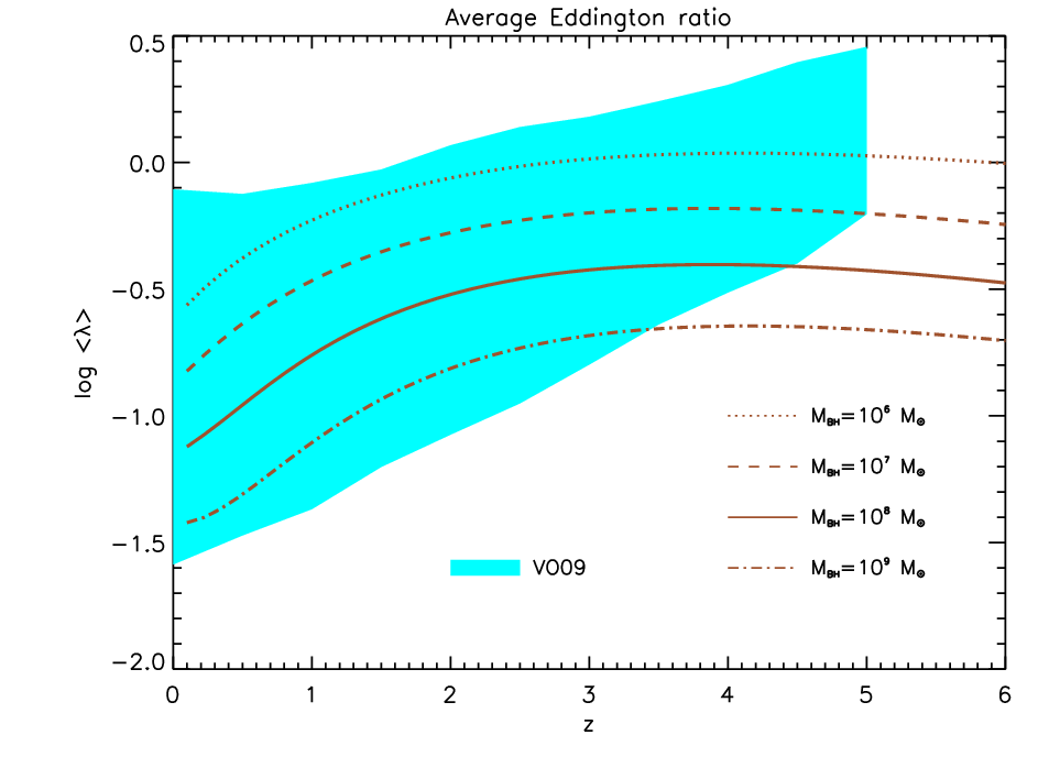


| function | ||||||||||||||||||||
|---|---|---|---|---|---|---|---|---|---|---|---|---|---|---|---|---|---|---|---|---|
| AGN LF | -3.80 | 0.45 | -1.00 | 0.00 | 10.90 | 1.10 | 6.94 | -11.55 | 1.40 | -1.70 | 3.40 | -1.75 | 0.36 | 0.62 | -1.59 | 0.8 | ||||
| SFR LF | -2.40 | -2.30 | 6.20 | -4.90 | 10.90 | 3.20 | -1.40 | -2.10 | 1.20 | 0.50 | -0.50 | 0.20 | 0.70 | -0.15 | 0.16 | 0.00 | ||||
| BH MF | -2.30 | -0.40 | -1.80 | -1.50 | 8.07 | -0.80 | 7.30 | -9.20 | 1.35 | -0.10 | 0.40 | 0.30 | 0.46 | 0.05 | 0.18 | -0.55 | ||||
| Stellar MF | -2.10 | -0.80 | 1.65 | -3.10 | 10.85 | 0.00 | 0.00 | -1.90 | 1.20 | 0.00 | -0.40 | 0.55 | 0.65 | 0.00 | -0.40 | 0.55 | ||||
| HMF | -3.97 | 0.00 | 0.00 | 1.50 | 14.00 | -0.90 | -1.90 | -1.10 | 1.80 | 0.50 | 0.10 | 0.70 | 0.47 | 0.45 | -0.10 | -0.45 | ||||
| GHMF | -3.35 | 0.50 | 0.1 | -1.50 | 13.05 | -0.80 | 0.00 | -1.30 | 1.88 | 0.30 | -0.40 | 1.30 | 1.10 | -0.10 | 0.00 | -0.43 | ||||
Note. — Typical tolerance on the parameters is less than . See Sect. II.1.1 for details on the redshift evolution of the parameters.
| function | ||||||||||||||||||||
|---|---|---|---|---|---|---|---|---|---|---|---|---|---|---|---|---|---|---|---|---|
| (1to1) | 12.25 | -1.90 | 1.45 | 1.10 | 12.30 | 0.00 | 0.00 | 0.00 | -1.65 | 1.20 | -4.50 | 0.60 | -0.65 | -3.50 | -0.40 | 0.80 | ||||
| (aver.) | 12.33 | -2.00 | 2.70 | -1.30 | 12.50 | 0.00 | 0.00 | 0.00 | -1.60 | 0.00 | -3.30 | 1.30 | -0.50 | -2.10 | -1.60 | 2.60 | ||||
| (aver.) | 11.25 | 0.00 | 0.00 | 0.00 | 12.20 | -1.20 | 0.00 | 0.00 | -1.30 | -3.00 | -0.50 | 1.20 | -0.50 | -1.50 | 0.00 | 1.50 | ||||
| (1to1) | 8.00 | -0.40 | 0.70 | -0.80 | 11.90 | 0.00 | 0.00 | 0.00 | -1.10 | -0.80 | -1.50 | 0.10 | -1.10 | -0.80 | -1.50 | 0.10 | ||||
| (aver.) | 8.20 | -0.20 | 0.80 | -1.50 | 12.20 | 0.00 | 0.00 | 0.00 | -1.40 | -1.30 | -0.30 | 0.10 | -0.80 | -0.40 | -1.10 | 0.10 | ||||
| (aver.) | 10.40 | -0.80 | 0.80 | -0.20 | 11.50 | 0.00 | 0.00 | 0.00 | -2.20 | -1.90 | -1.60 | 4.70 | -0.75 | -0.30 | -1.80 | 2.60 | ||||
| SFR (aver.) | 1.90 | 0.00 | 0.00 | 0.00 | 11.60 | -1.90 | -2.50 | 1.70 | -1.60 | 0.00 | 1.50 | -0.20 | -0.50 | -1.70 | 3.50 | -2.00 | ||||
| (1to1) | 7.33 | 0.10 | -0.70 | 1.00 | 10.60 | 0.00 | 0.00 | 0.00 | 1.60 | 0.00 | -0.20 | 2.80 | 0.60 | 0.40 | -0.40 | 2.20 | ||||
| (aver.) | 7.15 | 0.00 | -0.60 | 0.00 | 10.50 | 0.00 | 0.00 | 0.00 | 1.30 | 0.30 | 0.00 | 0.90 | 0.60 | 0.20 | 0.40 | 0.90 | ||||
Note. — Typical tolerance on the parameters is less than . See Appendix D for details on the redshift evolution of the parameters.
| Results | Sections | Figures | ||
|---|---|---|---|---|
| AGN luminosity function | II.1.1 | 1 | ||
| BH mass function | II.1 | 4 | ||
| SFR luminosity function | II.2.1 | 9 | ||
| Stellar mass function | II.2 | 10 | ||
| Galaxy halo mass function | III | 14 | ||
| relationship | III.1.1 | 15 | ||
| relationship | III.1.1 | 16 | ||
| AGN/BH bias | III.1.1 | 17 | ||
| relationship | III.1.2 | 18,19 | ||
| relationship | III.1.2 | 20 | ||
| Galaxy bias | III.1.2 | 21 | ||
| Cosmic sSFR vs. z | III.1.3 | 22 | ||
| sSFR vs. | III.1.3 | 23 | ||
| relationship | III.1.4 | 24 |