Implementing Scalable Boson Sampling with Time-Bin Encoding:
Analysis of Loss, Mode Mismatch, and Time Jitter

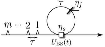
We will model loss inside of the inner fiber-loop with a beamsplitter of reflectivity $\eta_{f}$ and loss in the switch as $\eta_{s}$ as shown in Fig. 2. When $\eta_{f}=\eta_{s}=1$ the device has perfect efficiency. Before and after the inner loop the loss experienced by each mode in the fiber is negligible, since it may be arbitrarily short. Taking these losses into account, the implemented map of Eq. 5 becomes,

for a given loop, where $\eta=\eta_{f}\eta_{s}$. Note that this mapping is no longer a unitary matrix when $\eta_{f}<1$ or $\eta_{s}<1$. This uneven distribution of losses in the input-to-output mapping causes a skew in the matrix which prevents it from implementing the desired unitary transformation, even after post-selection.

In the full fiber-loop architecture $L$ inner loops are implemented via $L-1$ round-trips of the outer loop, before being coupled out to the detector. This architecture can implement an arbitrary unitary transformation when $L=m-1$ if there are no errors present. The outer loop and outer switches cause a uniform loss on the entire pulse-train, since every path through the interferometer passes through these elements the same number of times. Hence, these factor out of $\hat{U}$. The full lossy transformation that occurs is then,

where $L=m-1$ if an arbitrary transformation is desired, and $\hat{V}^{\prime}$ is given by Eq. 9. The ${\eta_{f}}^{m(L-1)}$ occurs because the pulse-train traverses an $m\tau$ length of fiber in the outer loop $L-1$ times (i.e $\eta_{f}$ can be regarded as the efficiency per unit of fiber of length $\tau$), and the ${\eta_{s}}^{2(L-1)}$ occurs because the pulse-train passes through the two outer switches $L-1$ times. Fig. 3 shows the entire architecture with these loss errors. For an example of loop bias due to loss see App. A. Extending from this loop bias example we generalize the loss matrix denoted as $\hat{\mathcal{L}}$, which represents the accumulation of losses in the fiber-loop architecture, as a function of the number of loops $L$ for an arbitrarily sized $m\times m$ transformation,

again where $\eta=\eta_{f}\eta_{s}$. Now the lossy map $\hat{U}^{\prime}$ may be written as an element wise product of the ideal unitary $\hat{U}$ and the loss matrix $\hat{\mathcal{L}}$,

Elements of $\hat{\mathcal{L}}$ that have no losses in them due to input modes not reaching output modes when $L<m-1$ will be accounted for appropriately when $\hat{\mathcal{L}}$ is multiplied by $\hat{U}$ by making the cooresponding matrix element in $\hat{U}^{\prime}$ go to zero.

In Fig. 4a we show how the optimised similarity with the uniform distribution varies with $\eta_{f}$ and $m$ for $L=m-1$ inner loops, one photon in all $m$ modes, and $\eta_{s}=1$. With low loss rates ($\eta_{f}\approx 1$) the implemented unitary remains highly uniform. However, with several loops the success probability of detecting all $n$ photons at the output decays exponentially as shown is Fig. 4b. For these plots the randomly generated $\hat{U}^{\prime}$ that maximises $\mathcal{S}$ for each $\eta_{f}$ and $m$ is used to calculate the corresponding $\mathcal{P}_{\mathrm{S}}$.

Now we consider how $\mathcal{S}$ and $\mathcal{P}_{\mathrm{S}}$ are affected in Fig. 5 with both the fiber loss and switch loss. We show this for the case of $m=3$ and one photon per input mode, which is in the regime of present-day demonstrations.

The temporal structure of a photon can be represented using a mode operator,

where $\psi(t-\Delta)$ is the temporal density function centered at time $t$, $\Delta$ is a shift of the temporal centre of the photon, and $\hat{a}^{{\dagger}}(t)$ is the time-dependent photon creation operator. This operator $\hat{\mathcal{A}}^{{\dagger}}(t,\Delta)$ acts on the vacuum $|0\rangle$ to create a photon with normalised Gaussian spectral density function,

where $c/\sqrt{2}$ is the standard deviation. We assume that $\tau\gg\Delta$, in which case $t$ denotes a time-bin, and $\Delta$ denotes a small mismatch within the respective time-bin, not large enough to cause a photon to ‘jump’ from one time-bin to the next. Thus, both $t$ and $\Delta$ represent shifts in the centre of the photon’s wavepacket, but the former is of the order of the time-bin separation, while the latter is of much smaller order than the time-bin separation.

To analyse mode-mismatch we will consider three regions of the architecture we label as $\mathcal{A}$, $\mathcal{B}$, and $\mathcal{C}$ as shown in Fig. 6. Region $\mathcal{A}$ corresponds to the modes that are input into the architecture from the source, region $\mathcal{B}$ corresponds to pulses inside the inner loop, and region $\mathcal{C}$ corresponds to pulses that exit the dynamic beamsplitter towards the detector. We introduce mode operators associated with each of these distinct regions — $\hat{\mathcal{A}}^{{\dagger}}(t,\Delta)$, $\hat{\mathcal{B}}^{{\dagger}}(t,\Delta)$, and $\hat{\mathcal{C}}^{{\dagger}}(t,\Delta)$ — each of the form of Eq. 13.

Since every pulse begins in region $\mathcal{A}$ the input state is a tensor product of pure states of the form,

where the tensor product is taken over all $m$ modes, $\{k\}$ is a known string representing the input photon-number configuration, and $k_{i}$ is number of photons in the $i$th input mode.

Next, the input state is transformed by the dynamic beamsplitter, which takes the mode-operators from region $\mathcal{A}$ into superpositions of regions $\mathcal{B}$ and $\mathcal{C}$,

and pulses from region $\mathcal{B}$ to superpositions of regions $\mathcal{B}$ and $\mathcal{C}$,

where we have used Eq. II for the elements of the dynamic beamsplitter at time $t$. $\hat{U}_{\mathrm{BS}}(t)$ only acts on photons arriving at the beamsplitter at time $t\pm\Delta$ since $\tau\gg\Delta$. When a photon enters the loop $t\to t+1$ as it advances to the next time-bin and will interfere with the next temporal mode. After this evolution, the entire pulse-train is coupled out of the loop such that the entire output state is a superposition of all possible output configurations.

Now we model the state of the pulse train after $t$ beam-splitters have been implemented,

where the integer values of $t$ denote the distinct time-bins. We note that there are $m+1$ total beam-splitters in a single implementation of the inner loop since there are $m-1$ beamsplitters to interfere the modes and another two beamsplitters to account for the initial and final boundary conditions of the MGDR protocol. Given how we modelled how the mode operators are transformed by $\hat{U}_{\mathrm{BS}}(t)$ in Eqs. 16 and 17 the $t$th beam-splitter acts on the mode operators only in modal position $t$. Since a pulse coming out of the inner loop exits at beam-splitter $t$ its modal position is $m=t-1$ which accounts for there being $m+1$ beam-splitters and $m$ modes.

In general the final evaluated form of $|\Psi_{\mathrm{out}}\rangle$ may be expressed as a superposition of all possible output photon-number configurations $S$, and their associated temporal configurations $T(S)$,

where $\gamma_{S,T}$ is the probability amplitude associated with photon time-bin configuration $S$ and temporal shift configuration $T(S)$, $t_{S_{i}}$ denotes the time-bin of the $i$th photon, $T(S)$ denotes a configuration of temporal shifts associated with the configuration $S$, and $\Delta_{T(S_{i})}$ is the temporal shift of the $i$th photon associated with configurations $S$ and $T$. This is the most general representation of a configuration of photons across time-bins with associated shifts. The probability of measuring a particular configuration is $|\gamma_{S,T}|^{2}$, and to evaluate these probabilities we must fully characterise spectrum of time-bin and temporal shift configurations, $S$ and $T$. Finding analytic forms for these expressions is largely prohibitive, and we calculate the $\gamma_{S,T}$ via brute-force simulation of the evolution of the mode-operators through the network as described earlier.

We analyse the results of this section by calculating the fidelity $\mathcal{F}$ between the ideal output state and the actual output state, given by,

where $|\Psi_{\mathrm{i}}\rangle$ is the ideal output state with no mode-mismatch ($\Delta\to 0$) and $|\Psi_{\mathrm{a}}\rangle$ is the actual output state obtained with mode-mismatch. $|\Psi_{\mathrm{a}}\rangle$ reduces to $|\Psi_{\mathrm{i}}\rangle$ in the limit of no errors yielding $\mathcal{F}=1$. Calculating this overlap but letting $|\Psi_{\mathrm{i}}\rangle$ have general temporal mode mismatch until the end of the calculation we obtain,

To simplify this expression further we use the formalism of second quantisation [24], which describes how the indistinguishability of particles in quantum mechanics undergo symmetrisation. Here we use the exchange symmetry of the bosonic Fock states, which accounts for how each temporal photon annihilation operator $\hat{\mathcal{C}}\big(t_{S^{\prime}_{i^{\prime}}},\Delta_{T^{\prime}(S_{i^{\prime}}^{\prime})}\big)$ overlaps with each temporal photon creation operator $\hat{\mathcal{C}}^{{\dagger}}\big(t_{S_{i}},\Delta_{T(S_{i})}\big)$. Using bosonic exchange symmetry we sum over all $m!$ permutations of $\bigotimes_{i^{\prime}=1}^{m}\hat{\mathcal{C}}\big(t_{S^{\prime}_{i^{\prime}}},\Delta_{S_{i^{\prime}}^{\prime}}\big)\bigotimes_{i=1}^{m}\hat{\mathcal{C}}^{{\dagger}}\big(t_{S_{i}},\Delta_{S_{i}}\big)$. Then Eq. 21 becomes,

where $\sigma$ are the permutations over $m$ elements.

Finally, to calculate $\mathcal{F}$ we must find the wave packet simplification for $\langle 0|\hat{\mathcal{C}}\big(t_{S^{\prime}_{\sigma_{i^{\prime}}}},\Delta_{T^{\prime}(S_{\sigma_{i^{\prime}}}^{\prime})}\big)\hat{\mathcal{C}}^{{\dagger}}\big(t_{S_{i}},\Delta_{T(S_{i})}|0\rangle$, which we perform in App. B. Using this result we obtain,

Letting the ideal state $|\Psi_{\mathrm{i}}\rangle$ have no temporal shifts, $\Delta\to 0$, this reduces to,

This derivation assumes the width of all wave-packets remain the same, i.e the photons are identical up to a temporal displacement. The width of the wave-packets may broaden due to dispersion but under the relatively short lengths of fiber-loop required for small $m$ the effect of dispersion may be neglected; however this formalism may be easily modified to include dispersion by creating an operator that broadens the wave-packet width $c$ as a function of the length of the fiber the wave-packet has traversed.

Next we consider two types of mode-mismatch: non-ideal lengths of the inner loop, and time-jitter at the input source.

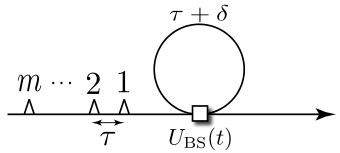
Here we analyse errors in the MGDR fiber-loop architecture caused by a non-ideal length of inner fiber-loop as shown in Fig. 7. We let the length of the inner loop have some length $\tau+\delta$, where $\delta$ is the error in the intended length $\tau$ and may be positive or negative. Thus every photon that traverses the inner loop acquires a temporal shift of $\delta$ from its expected centre. We ignore imperfect lengths of the outer loop because every mode will traverse the outer loop an equal number of times creating a global temporal shift with no impact on interference at the central beamsplitter.

The input state is given by Eq. 15 where $\Delta_{i}=0\ \forall\ i$. This models an ideal input state with no time-jitter or other errors in the source. To account for the unwanted time-delay $\delta$ we introduce the time-delay operator $\hat{\mathrm{T}}(\delta)$,

which acts only in region $\mathcal{B}$ – the region inside the inner loop. This adds a small temporal displacement, not enough to confuse time-bins. Thus it affects $\Delta$ but not $t$. It has no effect on the mode-operators $\hat{\mathcal{A}}$ and $\hat{\mathcal{C}}$. Using the boundary conditions shown in the MGDR protocol, the first photon is coupled completely into the loop so it picks up a time-delay of $\delta$. Afterwards the pulse-train interacts at the beamsplitter described in Eqs. 16 and 17, where it is sent into a superposition of regions $\mathcal{B}$ and $\mathcal{C}$. As the state evolves all amplitudes entering the inner loop (region $\mathcal{B}$) will acquire a time-shift of $\delta$. After the last mode traverses the inner loop the state is coupled completely out as per the MGDR protocol. The output state is given by,

where we have inserted the time-delay operator appropriately in Eq. 18. Fig. 8a shows how the fidelity $\mathcal{F}$ scales with $m$, $n$, and $\delta$ and Fig. 9b shows the worst- and best-case fidelities, where we have searched over switching sequences.

A major source of error in the time-bin architecture is time-jitter of the input source. Ideally each mode will be separated by time $\tau$ but in reality non-ideal sources will randomly shift modes from their desired centre of time $t_{i}$ in mode $i$. To model time-jitter we let the temporal shift of input mode $i$ be a Gaussian random variable $\epsilon_{i}$ drawn from the normal distribution,

centered in mode $i$ at time $t_{i}$ and with a standard deviation of $\sigma$. The input state of Eq. 15 becomes,

We assume that the shifts caused by time-jitter are much less than the time-bin separation $\tau$, such that the probability of time-bin confusion remains negligible, i.e. $\mathcal{N}(\epsilon_{i})\ll\tau$. Fig. 9a shows how the fidelity $\mathcal{F}$ scales with $m$, $n$, and $\sigma$. Fig. 9b shows the worst- and best-case $\mathcal{F}$, searching over many switching sequences.