跳到论文正文
W Papers独立论文阅读器 arXiv:1507.07145 论文正文 计算阅读时间 · 0%
引用这篇论文根据当前论文元数据生成,正式投稿前建议核对。


License: arXiv.org perpetual non-exclusive license
arXiv:1507.07145v1 [math.OC] 25 Jul 2015

Nearly convex sets: fine properties and domains or ranges of subdifferentials of convex functions

Sarah M. Moffat ††thanks: Mathematics, Irving K. Barber School, University of British Columbia Okanagan, Kelowna, British Columbia V1V 1V7, Canada. E-mail: sarah.moffat@ubc.ca.    Walaa M. Moursi ††thanks: Mathematics, Irving K. Barber School, University of British Columbia Okanagan, Kelowna, British Columbia V1V 1V7, Canada. E-mail: walaa.moursi@ubc.ca.    Xianfu Wang ††thanks: Mathematics, Irving K. Barber School, University of British Columbia Okanagan, Kelowna, British Columbia V1V 1V7, Canada. E-mail: shawn.wang@ubc.ca. Affiliation: Dedicated to R.T. Rockafellar on the occasion of his 80th birthday.
August 24, 2026
Abstract

Nearly convex sets play important roles in convex analysis, optimization and theory of monotone operators. We give a systematic study of nearly convex sets, and construct examples of subdifferentials of lower semicontinuous convex functions whose domain or ranges are nonconvex.

2000 Mathematics Subject Classification: Primary 52A41, 26A51, 47H05; Secondary 47H04, 52A30, 52A25.

Keywords: Maximally monotone operator, nearly convex set, nearly equal, relative interior, recession cone, subdifferential with nonconvex domain or range.

1 Introduction

In 1960s Minty and Rockafellar coined nearly convex sets [22, 25]. Being a generalization of convex sets, the notion of near convexity or almost convexity has been gaining popularity in the optimization community, see [6, 11, 12, 13, 16]. This can be attributed to the applications of generalized convexity in economics problems, see for example, [19, 21]. One reason to study nearly convex sets is that for a proper lower semicontinuous convex function its subdifferential domain is always nearly convex [24, Theorem 23.4, Theorem 6.1], and the same is true for the domain of each maximally monotone operator [26, Theorem 12.41]. Maximally monotone operators are extensively studies recently [1, 2, 3, 4, 27]. Another reason is that to study possibly nonconvex functions, a first endeavor perhaps should be to study functions whose epigraphs are nearly convex, see, e.g., [13].

All these motivate our systematic study of nearly convex sets. Some properties of nearly convex sets have been partially studied in [6, 11, 12, 13] from different perspectives. The purpose of this paper is to give new proofs to some known results, provide further characterizations, and extend known results on calculus, relative interiors, recession cones, and applications. Although nearly convex sets need not be convex, many results on convex sets do extend. We also construct proper lower semicontinuous convex functions whose subdifferential mappings have domains being neither closed nor open; or highly nonconvex.

We remark that nearly convex was called almost convex in [11, 12, 13]. Here, we adopt the term nearly convex rather than almost convex because of the relationship with nearly equal sets which was noted in [6]. Note that this definition of nearly convex does not coincide with the one provided in [11, Definition 2] and [12], where nearly convex is a generalization of midpoint convexity.

The remainder of the paper is organized as follows. Some basic notations and facts about convex sets and nearly convex sets are given in Section 2. Section 3 gives new characterizations of nearly convex sets. In Section 4, we give calculus of nearly convex sets and relative interiors. In Section 5, we study recessions of nearly convex sets. Section 6 is devoted to apply results in Section 4 and Section 5 to study maximality of sum of several maximally monotone operators and closedness of nearly convex sets under a linear mapping. In Section 7, we construct examples of proper lower semicontinuous convex functions with prescribed nearly convex sets being their subdifferential domain. As early as 1970s, Rockafellar provided a convex function whose subdifferential domain is not convex [24]. We give a detailed analysis of his classical example and use it to generate new examples with pathological subdifferential domains. Open problems appear in Section 8. Appendix A contains some proofs of Section 7.

2 Preliminaries

2.1 Notation and terminology

Throughout this paper, we work in the Euclidean space ℝn\mathbb{R}^{n} with norm ∥⋅∥\|\cdot\| and inner product ⟨⋅,⋅⟩\langle\cdot,\cdot\rangle. For a set C⊆ℝnC\subseteq\mathbb{R}^{n} let cl⁡C\operatorname{cl}{C} denote the closure of CC, and aff⁡C\operatorname{aff}C the affine hull of CC; that is, the smallest affine set containing CC. The key object we shall study is:

Definition 2.1 (near convexity)

A set E⊆ℝnE\subseteq\mathbb{R}^{n} is nearly convex if there exists a convex set C⊆ℝnC\subseteq\mathbb{R}^{n} such that

C⊆E⊆cl⁡C.C\subseteq E\subseteq\operatorname{cl}{C}.

Obviously, every convex set is nearly convex, but they are many nearly convex sets which are not convex. See Figure 1 for two nearly convex sets.

Refer to caption Refer to caption
Figure 1: A GeoGebra [17] snapshot. Left: Neither open nor closed convex set. Right: Nearly convex but not convex set

Note that nearly convex sets do not have nice algebra as convex sets do [24, Section 3], as the following two simple examples illustrate.

Example 2.2

The nearly convex set C⊆ℝ2C\subseteq\mathbb{R}^{2} given by

C:={(x1,x2)∣−1<x1​<1,x2>​0}∪{(−1,0),(1,0)}.C:=\big\{{(x_{1},x_{2})}\mid{-1<x_{1}<1,x_{2}>0}\big\}\cup\{(-1,0),(1,0)\}.

has 2​C≠C+C2C\neq C+C, since

2​C\displaystyle 2C ={(x1,x2)∣−2<x1​<2,x2>​0}∪{(−2,0),(2,0)},\displaystyle=\big\{{(x_{1},x_{2})}\mid{-2<x_{1}<2,x_{2}>0}\big\}\cup\{(-2,0),(2,0)\},
C+C\displaystyle C+C =2​C∪(0,0).\displaystyle=2C\cup{(0,0)}.

On the contrary, 2​C=C+C2C=C+C whenever CC is a convex set [24, Theorem 3.2].

Example 2.3

Define

E1:={(x1,x2)∣x1≥0,x2∈ℝ}∖{(0,x2)∣|x2|<1},E_{1}:=\big\{{(x_{1},x_{2})}\mid{x_{1}\geq 0,x_{2}\in\mathbb{R}}\big\}\setminus\big\{{(0,x_{2})}\mid{|x_{2}|<1}\big\},
E2:={(x1,x2)∣x1≤0,x2∈ℝ}∖{(0,x2)∣|x2|<1}.E_{2}:=\big\{{(x_{1},x_{2})}\mid{x_{1}\leq 0,x_{2}\in\mathbb{R}}\big\}\setminus\big\{{(0,x_{2})}\mid{|x_{2}|<1}\big\}.

The set E1∩E2={(0,x2)∣|x2|≥1}E_{1}\cap E_{2}=\big\{{(0,x_{2})}\mid{|x_{2}|\geq 1}\big\} is not nearly convex. On the contrary, E1∩E2E_{1}\cap E_{2} is convex if both E1,E2E_{1},E_{2} are convex.

Let B⁡(x,ε)⊂ℝnB(x,\varepsilon)\subset\mathbb{R}^{n} be the closed ball with radius ε>0\varepsilon>0 and centered at xx, and let II be an index set I:={1,2,…,m}I:=\{1,2,\dots,m\} for some integer mm. We use conv⁡C\operatorname{conv}C for the convex hull of CC. The interior of CC is int⁡C\operatorname{int}C, the core is

core⁡C:={x∈C|(∀y∈ℝn)​(∃ε>0)​[x−ε​y,x+ε​y]⊆C},\operatorname{core}C:=\{x\in C\;|\;(\forall y\in\mathbb{R}^{n})(\exists\varepsilon>0)\left[x-\varepsilon y,x+\varepsilon y\right]\subseteq C\},

and the relative interior is

riC:={x∈affC|∃ε>0,(x+εB(0,1))∩(affC)⊆C}.\operatorname{ri}C:=\{x\in\operatorname{aff}C\;|\;\exists\varepsilon>0,(x+\varepsilon B(0,1))\cap(\operatorname{aff}C)\subseteq C\}.

The recession cone of CC is

rec⁡C:={y∈ℝn|(∀λ≥0)​λ​y+C⊆C}.\operatorname{rec}C:=\{y\in\mathbb{R}^{n}\;|\;(\forall\lambda\geq 0)~\lambda y+C\subseteq C\}. (1)

The lineality space of CC is the largest subspace contained in rec⁡C\operatorname{rec}C, see [24, page 65] for more on lineality spaces. We denote the projection operator onto the set C⊆ℝnC\subseteq\mathbb{R}^{n} by PCP_{C} and the normal cone operator by NCN_{C}.

For a set-valued mapping A:ℝn⇉ℝnA:\mathbb{R}^{n}\rightrightarrows\mathbb{R}^{n}, the domain is dom⁡A:={x∈ℝn|A​x≠∅}\operatorname{dom}A:=\{x\in\mathbb{R}^{n}\;|\;Ax\neq\varnothing\}, the range is ran⁡A:=⋃x∈ℝnA​x,\operatorname{ran}A:=\bigcup_{x\in\mathbb{R}^{n}}Ax, and the graph is gra⁡A:={(x,u)∈ℝn×ℝn|u∈A​x}.\operatorname{gra}A:=\{(x,u)\in\mathbb{R}^{n}\times\mathbb{R}^{n}\;|\;u\in Ax\}. AA is monotone if (∀(x,u)∈gra⁡A)​(∀(y,v)∈gra⁡A)⟨x−y,u−v⟩≥0(\forall(x,u)\in\operatorname{gra}A)(\forall(y,v)\in\operatorname{gra}A)\quad\langle{{x-y},{u-v}}\rangle\geq 0, and maximally monotone if there exists no monotone operator BB such that gra⁡A\operatorname{gra}A is a proper subset of gra⁡B\operatorname{gra}B.

2.2 Auxiliary results on convex sets

Properties of convex sets play a prominent role in the paper, we need to review some key results.

Fact 2.4 (Rockafellar)

Let CC and DD be convex subsets of ℝn\mathbb{R}^{n}, and let λ∈ℝ\lambda\in\mathbb{R}. Then the following hold:

  1. (i)

    ri⁡C\operatorname{ri}C and cl⁡C\operatorname{cl}{C} are convex.

  2. (ii)

    C≠∅C\neq\varnothing ⇒\Rightarrow ri⁡C≠∅\operatorname{ri}C\neq\varnothing.

  3. (iii)

    cl⁡(ri⁡C)=cl⁡C\operatorname{cl}{(\operatorname{ri}C)}=\operatorname{cl}{C}.

  4. (iv)

    ri⁡C=ri⁡(cl⁡C)\operatorname{ri}C=\operatorname{ri}(\operatorname{cl}{C}).

  5. (v)

    aff⁡(ri⁡C)=aff⁡C=aff⁡(cl⁡C)\operatorname{aff}(\operatorname{ri}C)=\operatorname{aff}C=\operatorname{aff}(\operatorname{cl}{C}).

  6. (vi)

    ri⁡C=ri⁡D\operatorname{ri}C=\operatorname{ri}D ⇔\Leftrightarrow cl⁡C=cl⁡D\operatorname{cl}{C}=\operatorname{cl}{D} ⇔\Leftrightarrow ri⁡C⊆D⊆cl⁡C\operatorname{ri}C\subseteq D\subseteq\operatorname{cl}{C}.

  7. (vii)

    ri⁡λ​C=λ​ri⁡C\operatorname{ri}\lambda C=\lambda\operatorname{ri}C.

  8. (viii)

    ri⁡(C+D)=ri⁡C+ri⁡D.\operatorname{ri}(C+D)=\operatorname{ri}C+\operatorname{ri}D.

Proof. (i)&(ii): See [24, Theorem 6.2]. (iii)&(iv): See [24, Theorem 6.3]. (v): See [24, Theorem 6.2]. (vi): See [24, Corollary 6.3.1]. (vii): See [24, Corollary 6.6.1]. (viii): See [24, Corollary 6.6.2]. ■\quad\hfill\blacksquare

Fact 2.5

[24, Theorem 6.5] Let CiC_{i} be a convex set in ℝn\mathbb{R}^{n} for i=1,…,mi=1,\ldots,m such that ⋂i=1mri⁡Ci≠∅\bigcap\limits_{i=1}^{m}\operatorname{ri}C_{i}\neq\varnothing. Then

cl⁡(⋂i=1mCi)=⋂i=1mcl⁡Ci,\operatorname{cl}{\big(\bigcap\limits_{i=1}^{m}C_{i}\big)}=\bigcap\limits_{i=1}^{m}\operatorname{cl}{C_{i}},

and

ri⁡(⋂i=1mCi)=⋂i=1mri⁡Ci.\operatorname{ri}\big(\bigcap\limits_{i=1}^{m}C_{i}\big)=\bigcap\limits_{i=1}^{m}\operatorname{ri}C_{i}.
Fact 2.6

[24, Theorem 6.1] Let CC be a convex set in ℝn\mathbb{R}^{n}, x∈ri⁡Cx\in\operatorname{ri}C, and y∈cl⁡Cy\in\operatorname{cl}{C}. Then

[x,y[⊆riC.[x,y[\subseteq\operatorname{ri}C.
Fact 2.7

[24, Theorem 6.6] Let CC be a convex set in ℝn\mathbb{R}^{n} and let AA be a linear transformation from ℝn\mathbb{R}^{n} to ℝm\mathbb{R}^{m}. Then

ri⁡(A​C)=A⁡(ri⁡C),\operatorname{ri}(AC)=A(\operatorname{ri}C),

and

A⁡(cl⁡C)⊆cl⁡(A​C).A(\operatorname{cl}{C})\subseteq\operatorname{cl}{(AC)}.
Fact 2.8

[24, Theorem 6.7] Let CC be a convex set in ℝn\mathbb{R}^{n} and let AA be a linear transformation from ℝn\mathbb{R}^{n} to ℝm\mathbb{R}^{m} such that A−1​(ri⁡C)≠∅A^{-1}(\operatorname{ri}C)\neq\varnothing. Then

ri⁡(A−1​C)=A−1​(ri⁡C),\operatorname{ri}(A^{-1}C)=A^{-1}(\operatorname{ri}C),

and

cl⁡(A−1​C)=A−1​(cl⁡C).\operatorname{cl}{({A^{-1}C})}=A^{-1}(\operatorname{cl}{C}).
Fact 2.9

[24, Theorem 8.1 & Theorem 8.2] Let CC be a nonempty convex subset in ℝn\mathbb{R}^{n}. Then rec⁡C\operatorname{rec}C is a convex cone and 0∈rec⁡C0\in\operatorname{rec}C. If in addition CC is closed then rec⁡C\operatorname{rec}C is closed.

Fact 2.10

[24, Theorem 8.3] Let CC be a nonempty convex subset in ℝn\mathbb{R}^{n}. Then rec⁡(ri⁡C)=rec⁡(cl⁡C)\operatorname{rec}(\operatorname{ri}C)=\operatorname{rec}(\operatorname{cl}{C}).

Fact 2.11

[24, Theorem 9.1] Let CC be a nonempty convex subset in ℝn\mathbb{R}^{n} and let AA be a linear transformation from ℝn\mathbb{R}^{n} to ℝm\mathbb{R}^{m}. Suppose that (∀z∈rec⁡(cl⁡C)∖{0})(\forall z\in\operatorname{rec}(\operatorname{cl}{C})\setminus\left\{0\right\}) with A​z=0Az=0 we have that zz belongs to the lineality space of cl⁡C\operatorname{cl}{C}. Then

cl⁡(A​C)=A⁡(cl⁡C),\operatorname{cl}{(AC)}=A(\operatorname{cl}{C}),

and

rec⁡A⁡(cl⁡C)=A⁡[rec⁡(cl⁡C)].\operatorname{rec}A(\operatorname{cl}{C})=A[\operatorname{rec}(\operatorname{cl}{C})].
Fact 2.12

[24, Corollary 9.1.1] Let (Ei)i∈I(E_{i})_{i\in I}, be a family of nonempty convex subsets in ℝn\mathbb{R}^{n} satisfying the following condition: if (∀i∈I)​(∃zi∈rec⁡(cl⁡Ei))(\forall i\in I)(\exists z_{i}\in\operatorname{rec}(\operatorname{cl}{E_{i}})) and ∑i∈Izi=0\sum_{i\in I}z_{i}=0 then (∀i∈I)​zi(\forall i\in I)z_{i} belongs to the lineality space of cl⁡Ei\operatorname{cl}{E_{i}}. Then

cl⁡(E1+⋯+Em)\displaystyle\operatorname{cl}{(E_{1}+\cdots+E_{m})} =cl⁡E1+⋯+cl⁡Em,\displaystyle=\operatorname{cl}{E_{1}}+\cdots+\operatorname{cl}{E_{m}}, (2)
rec⁡[cl⁡(E1+⋯+Em)]\displaystyle\operatorname{rec}[\operatorname{cl}{(E_{1}+\cdots+E_{m})}] =rec⁡(cl⁡E1)+⋯+rec⁡(cl⁡Em).\displaystyle=\operatorname{rec}(\operatorname{cl}{E_{1}})+\cdots+\operatorname{rec}(\operatorname{cl}{E_{m}}). (3)

2.3 Auxiliary results on nearly convex sets

Near equality introduced in [6] provides a convenient tool to study nearly convex sets and ranges of maximally monotone operators.

Definition 2.13 (near equality)

Let CC and DD be subsets of ℝn\mathbb{R}^{n}. We say that CC and DD are nearly equal, if

cl⁡C=cl⁡D​ and ​ri⁡C=ri⁡D.\operatorname{cl}{C}=\operatorname{cl}{D}\text{ and }\operatorname{ri}C=\operatorname{ri}D. (4)

and denote this by C≈DC\approx D.

Fact 2.14

[6, Lemma 2.7] Let EE be a nearly convex subset of ℝn\mathbb{R}^{n}, say C⊆E⊆cl⁡CC\subseteq E\subseteq\operatorname{cl}{C}, where CC is a convex subset of ℝn\mathbb{R}^{n}. Then

E≈cl⁡E≈ri⁡E≈conv⁡E≈ri⁡conv⁡E≈C.E\approx\operatorname{cl}{E}\approx\operatorname{ri}E\approx\operatorname{conv}E\approx\operatorname{ri}\operatorname{conv}E\approx C. (5)

In particular, the following hold.

  1. (i)

    cl⁡E\operatorname{cl}{E} and ri⁡E\operatorname{ri}E are convex.

  2. (ii)

    If E≠∅E\neq\varnothing, then ri⁡E≠∅\operatorname{ri}E\neq\varnothing.

Fact 2.15

[6, Proposition 2.12(i),(ii),(iii)] Let E1E_{1} and E2E_{2} be nearly convex subsets of ℝn\mathbb{R}^{n}. Then

E1≈E2⇔ri⁡E1=ri⁡E2⇔cl⁡E1=cl⁡E2.E_{1}\approx E_{2}\Leftrightarrow\operatorname{ri}E_{1}=\operatorname{ri}E_{2}\Leftrightarrow\operatorname{cl}{E_{1}}=\operatorname{cl}{E_{2}}. (6)
Fact 2.16

[6, Proposition 2.5] Let AA, BB and CC be subsets of ℝn\mathbb{R}^{n} such that A≈CA\approx C and A⊆B⊆CA\subseteq B\subseteq C. Then A≈B≈CA\approx B\approx C.

Fact 2.17

(See [26, Theorem 12.41].) Let A:ℝn⇉ℝnA:\mathbb{R}^{n}\rightrightarrows\mathbb{R}^{n} be maximally monotone. Then dom⁡A\operatorname{dom}A and ran⁡A\operatorname{ran}A are nearly convex.

Remark 2.18

Fact 2.17 can not be localized. Suppose that A:=PB⁡(0,1)A:=P_{B(0,1)} is the projection onto the unit ball in ℝ2\mathbb{R}^{2}, which is a gradient mapping of the continuous differentiable convex function f:ℝ2→ℝf:\mathbb{R}^{2}\rightarrow\mathbb{R} given by

f⁡(x):={‖x‖2/2 if ‖x‖≤1,‖x‖−1/2 if ‖x‖>1.f(x):=\begin{cases}\|x\|^{2}/2&\text{ if $\|x\|\leq 1$,}\\ \|x\|-1/2&\text{ if $\|x\|>1$.}\end{cases}
  1. (i)

    Let S:={(x,y)∈ℝ2∣x+y>2,x>0,y>0}S:=\big\{{(x,y)\in\mathbb{R}^{2}}\mid{x+y>2,x>0,y>0}\big\} be open convex. The set ranPB⁡(0,1)(S)={(x,y)∈ℝ2∣x2+y2=1,x>0,y>0}\operatorname{ran}P_{B(0,1)}(S)=\big\{{(x,y)\in\mathbb{R}^{2}}\mid{x^{2}+y^{2}=1,x>0,y>0}\big\} is not nearly convex.

  2. (ii)

    Let S:={(x,y)∈ℝ2∣x+y≥2,x≥0,y≥0}S:=\big\{{(x,y)\in\mathbb{R}^{2}}\mid{x+y\geq 2,x\geq 0,y\geq 0}\big\} be closed convex. The set ranPB⁡(0,1)(S)={(x,y)∈ℝ2∣x2+y2=1,x≥0,y≥0}\operatorname{ran}P_{B(0,1)}(S)=\big\{{(x,y)\in\mathbb{R}^{2}}\mid{x^{2}+y^{2}=1,x\geq 0,y\geq 0}\big\} is not nearly convex.

We refer readers to [9, 10, 4, 24, 27] for more materials on convex analysis and monotone operators.

3 Characterizations and basic properties of nearly convex sets

Utilizing near equality, in [6] the authors provide the following characterizations of nearly convex sets.

Fact 3.1 (characterization of near convexity)

[6, Lemma 2.9] Let E⊆ℝnE\subseteq\mathbb{R}^{n}. Then the following are equivalent:

  1. (i)

    EE is nearly convex.

  2. (ii)

    E≈conv⁡EE\approx\operatorname{conv}E.

  3. (iii)

    EE is nearly equal to a convex set.

  4. (iv)

    EE is nearly equal to a nearly convex set.

  5. (v)

    ri⁡conv⁡E⊆E\operatorname{ri}\operatorname{conv}E\subseteq E.

We now provide further characterizations of nearly convex sets.

Theorem 3.2

Let EE be a nonempty subset of ℝn\mathbb{R}^{n}. Then the following are equivalent:

  1. (i)

    EE is nearly convex.

  2. (ii)

    ri⁡E\operatorname{ri}E is convex and cl⁡(ri⁡E)=cl⁡E\operatorname{cl}{(\operatorname{ri}E)}=\operatorname{cl}{E}.

  3. (iii)

    (∀x∈ri⁡E)(\forall x\in\operatorname{ri}E) (∀y∈E)(\forall y\in E) [x,y[⊆riE[x,y[\subseteq\operatorname{ri}E.

  4. (iv)

    cl⁡E\operatorname{cl}{E} is convex and ri⁡(cl⁡E)⊆ri⁡E\operatorname{ri}(\operatorname{cl}{E})\subseteq\operatorname{ri}{E}.

Proof. (i)⇒\Rightarrow(ii): This follows from Fact 2.14. (ii)⇒\Rightarrow(i): We have ri⁡E⊆E⊆E¯=cl⁡(ri⁡E)\operatorname{ri}E\subseteq E\subseteq\overline{E}=\operatorname{cl}{(\operatorname{ri}E)}. Since ri⁡E\operatorname{ri}E is convex, EE is nearly convex. (ii)⇒\Rightarrow(iii): Since EE is nearly convex, by Fact 2.14(i) cl⁡E\operatorname{cl}{E} is convex. Using Fact 2.6 applied to the convex set cl⁡E\operatorname{cl}{E} we conclude that (∀x∈ri⁡E)(\forall x\in\operatorname{ri}E) (∀y∈cl⁡E)(\forall y\in\operatorname{cl}{E}) [x,y[⊆ri(clE)=riE[x,y[\subseteq\operatorname{ri}(\operatorname{cl}{E})=\operatorname{ri}E. In particular, (∀x∈ri⁡E)(\forall x\in\operatorname{ri}E) (∀y∈E)(\forall y\in E) [x,y[⊆riE[x,y[\subseteq\operatorname{ri}E. (iii)⇒\Rightarrow(ii): Let x∈ri⁡Ex\in\operatorname{ri}E and y∈ri⁡Ey\in\operatorname{ri}E. Then [x,y]=[x,y[∪{y}⊆riE∪riE=riE[x,y]=[x,y[~\cup\left\{y\right\}\subseteq\operatorname{ri}E\cup\operatorname{ri}E=\operatorname{ri}E, that is ri⁡E\operatorname{ri}E is convex. It is obvious that cl⁡(ri⁡E)⊆cl⁡E\operatorname{cl}{(\operatorname{ri}E)}\subseteq\operatorname{cl}{E}. Now we show that cl⁡E⊆cl⁡(ri⁡E)\operatorname{cl}{E}\subseteq\operatorname{cl}{(\operatorname{ri}E)}. Indeed, let y∈cl⁡Ey\in\operatorname{cl}{E}. Then (∃(yn)n∈ℕ)⊆E(\exists(y_{n})_{n\in\mathbb{N}})\subseteq E such that yn→yy_{n}\to y. Therefore (∀x∈ri⁡E)(\forall x\in\operatorname{ri}E) [x,yn[⊆riE[x,y_{n}[\subseteq\operatorname{ri}E, and consequently [x,yn]⊆cl⁡(ri⁡E)[x,y_{n}]\subseteq\operatorname{cl}{(\operatorname{ri}E)}. That is, (yn)n∈ℕ⊆cl⁡(ri⁡E)(y_{n})_{n\in\mathbb{N}}\subseteq\operatorname{cl}(\operatorname{ri}E), hence y∈cl⁡(ri⁡E)y\in\operatorname{cl}{(\operatorname{ri}E)}, and therefore cl⁡E⊆cl⁡(ri⁡E)\operatorname{cl}{E}\subseteq\operatorname{cl}{(\operatorname{ri}E)}, as claimed. (i)⇒\Rightarrow(iv): This follows from Fact 2.14. (iv)⇒\Rightarrow(i): Since EE is nonempty we have cl⁡E\operatorname{cl}{E} is nonempty and convex by assumption, hence cl⁡[ri⁡(cl⁡E)]=cl⁡E\operatorname{cl}{[\operatorname{ri}(\operatorname{cl}{E})]}=\operatorname{cl}{E}. Now ri⁡(cl⁡E)⊆ri⁡E⊆E⊆cl⁡E=cl⁡[ri⁡(cl⁡E)]\operatorname{ri}(\operatorname{cl}{E})\subseteq\operatorname{ri}E\subseteq E\subseteq\operatorname{cl}{E}=\operatorname{cl}{[\operatorname{ri}(\operatorname{cl}{E})]}, hence ri⁡(cl⁡E)≈E\operatorname{ri}(\operatorname{cl}{E})\approx E. Since cl⁡E\operatorname{cl}{E} is convex we have ri⁡(cl⁡E)\operatorname{ri}(\operatorname{cl}{E}) is convex. It follows from Fact 3.1(iii) that EE is nearly convex. ■\quad\hfill\blacksquare

Theorem 3.3

Let EE be a nonempty subset in ℝn\mathbb{R}^{n}. Then EE is nearly convex if and only if E=C∪SE=C\cup S where CC is a nonempty convex subset of ℝn\mathbb{R}^{n} and S⊆cl⁡C∖ri⁡CS\subseteq\operatorname{cl}{C}\setminus\operatorname{ri}C.

Proof. (⇒)(\Rightarrow) Suppose that EE is nearly convex, and notice that E=ri⁡E∪(E∖ri⁡E)E=\operatorname{ri}E\cup(E\setminus\operatorname{ri}E). Set

C:=ri⁡E​and​S:=E∖ri⁡E⊆cl⁡E∖ri⁡E.C:=\operatorname{ri}E\;\;\;\text{and}\;\;\;S:=E\setminus\operatorname{ri}E\subseteq\operatorname{cl}{E}\setminus\operatorname{ri}E. (7)

Since EE is nearly convex, it follows from Fact 2.14 that CC is nonempty and convex. Moreover cl⁡E=cl⁡(ri⁡E)=cl⁡C\operatorname{cl}{E}=\operatorname{cl}{(\operatorname{ri}E)}=\operatorname{cl}{C}. Therefore E=C∪SE=C\cup S with CC convex and S⊆cl⁡C∖ri⁡CS\subseteq\operatorname{cl}{C}\setminus\operatorname{ri}C. (⇐)(\Leftarrow) Conversely, assume that E=C∪SE=C\cup S where CC is a nonempty convex subset of ℝn\mathbb{R}^{n} and S⊆cl⁡C∖ri⁡CS\subseteq\operatorname{cl}{C}\setminus\operatorname{ri}C. Clearly, S⊆∂(cl⁡C)S\subseteq{\partial}(\operatorname{cl}{C}), where ∂(cl⁡C){\partial}(\operatorname{cl}{C}) is the relative boundary of cl⁡C\operatorname{cl}{C}. Hence ri⁡E=ri⁡C\operatorname{ri}E=\operatorname{ri}C and consequently ri⁡E\operatorname{ri}E is nonempty and convex. Moreover, since cl⁡S⊆cl⁡C\operatorname{cl}{S}\subseteq\operatorname{cl}{C}, we have cl⁡E=cl⁡(C∪S)=cl⁡C∪cl⁡S=cl⁡C\operatorname{cl}{E}=\operatorname{cl}{(C\cup S)}=\operatorname{cl}{C}\cup\operatorname{cl}{S}=\operatorname{cl}{C} and consequently cl⁡E\operatorname{cl}{E} is convex. Finally notice that

ri⁡C=ri⁡E⊆E⊆cl⁡E=cl⁡C=cl⁡(ri⁡C).\operatorname{ri}C=\operatorname{ri}E\subseteq E\subseteq\operatorname{cl}{E}=\operatorname{cl}{C}=\operatorname{cl}{(\operatorname{ri}C)}. (8)

That is E≈ri⁡CE\approx\operatorname{ri}C and hence EE is nearly convex by Fact 3.1(iii). ■\quad\hfill\blacksquare

To study the relationship among core, interior and relative interior of a nearly convex set, we need two facts.

Fact 3.4

Let CC be a convex set in ℝn\mathbb{R}^{n}. Then int⁡C=core⁡C\operatorname{int}C=\operatorname{core}C. Moreover, if int⁡C≠∅\operatorname{int}C\neq\varnothing then int⁡C=ri⁡C\operatorname{int}C=\operatorname{ri}C.

Proof. For the first part, see [8, Remark 2.73] or [4, Proposition 6.12]. The second part is clear from [24, pg 44]. ■\quad\hfill\blacksquare

Fact 3.5

[6, Proposition 2.20] Let EE be a nearly convex subset of ℝn\mathbb{R}^{n}. Then int⁡E=int⁡(cl⁡E)\operatorname{int}E=\operatorname{int}(\operatorname{cl}{E}).

Theorem 3.6

Let EE be a nonempty nearly convex subset in ℝn\mathbb{R}^{n}. Then the following hold:

  1. (i)

    core⁡E=int⁡E\operatorname{core}E=\operatorname{int}E.

  2. (ii)

    If int⁡E≠∅\operatorname{int}E\neq\varnothing then int⁡E=ri⁡E\operatorname{int}E=\operatorname{ri}E.

  3. (iii)

    aff⁡(ri⁡E)=aff⁡E=aff⁡(cl⁡E)\operatorname{aff}(\operatorname{ri}E)=\operatorname{aff}E=\operatorname{aff}(\operatorname{cl}{E}).

Proof. (i): Since EE is nonempty and nearly convex, cl⁡E\operatorname{cl}{E} is nonempty and convex by Fact 2.14(i). Using Fact 3.5 and Fact 3.4 applied to the convex set cl⁡E\operatorname{cl}{E} we have

int⁡(cl⁡E)=int⁡E⊆core⁡E⊆core⁡(cl⁡E)=int⁡(cl⁡E).\operatorname{int}(\operatorname{cl}{E})=\operatorname{int}E\subseteq\operatorname{core}E\subseteq\operatorname{core}(\operatorname{cl}{E})=\operatorname{int}(\operatorname{cl}{E}). (9)

Hence int⁡E=core⁡E\operatorname{int}E=\operatorname{core}E, as claimed.

(ii): Notice that Fact 3.5 gives ∅≠int⁡E=int⁡(cl⁡E)\varnothing\neq\operatorname{int}E=\operatorname{int}(\operatorname{cl}{E}). Moreover since EE is nearly convex, Fact 2.14 implies that ri⁡E=ri⁡(cl⁡E)\operatorname{ri}E=\operatorname{ri}(\operatorname{cl}{E}). Applying Fact 3.4 to the convex set cl⁡E\operatorname{cl}{E} gives

int⁡E=int⁡(cl⁡E)=ri⁡(cl⁡E)=ri⁡E.\operatorname{int}E=\operatorname{int}(\operatorname{cl}{E})=\operatorname{ri}(\operatorname{cl}{E})=\operatorname{ri}E. (10)

(iii): It follows from Fact 2.14 that

ri⁡E=ri⁡(ri⁡E)​and​cl⁡(ri⁡E)=cl⁡E.\operatorname{ri}E=\operatorname{ri}(\operatorname{ri}E)\;\;\;\text{and}\;\;\;\operatorname{cl}{(\operatorname{ri}E)}=\operatorname{cl}{E}. (11)

Using (11) and Fact 2.4(v) applied to the convex set ri⁡E\operatorname{ri}E we have

aff⁡(ri⁡E)=aff⁡[cl⁡(ri⁡E)]=aff⁡(cl⁡E).\operatorname{aff}(\operatorname{ri}E)=\operatorname{aff}[\operatorname{cl}{(\operatorname{ri}E)}]=\operatorname{aff}(\operatorname{cl}{E}). (12)

■\quad\hfill\blacksquare

Under mild assumptions, a nearly convex set is in fact convex as our next result shows.

Definition 3.7

We say that a set E⊆XE\subseteq X is relatively strictly convex if ]x,y[⊆ri⁡E]x,y[\subseteq\operatorname{ri}E whenever x,y∈Ex,y\in E.

Proposition 3.8

Let E⊆ℝnE\subseteq\mathbb{R}^{n} be nearly convex. Then the following hold:

  1. (i)

    If EE is relatively strictly convex, then EE is convex.

  2. (ii)

    If EE is open, then EE is convex.

  3. (iii)

    If EE is closed, then EE is convex.

  4. (iv)

    If for every x,y∈E∖ri⁡Ex,y\in E\setminus\operatorname{ri}E, we have [x,y]⊆E[x,y]\subseteq E, then EE is convex.

Proof. (i): Let x,y∈Ex,y\in E. As EE is relatively strictly convex, ]x,y[⊆ri⁡E⊆E]x,y[\subseteq\operatorname{ri}E\subseteq E, so [x,y]⊆E[x,y]\subseteq E. Hence EE is convex.

(ii): For a nearly convex set EE, we have ri⁡E=ri⁡C\operatorname{ri}E=\operatorname{ri}C where CC is a convex set. When EE is open and int⁡E≠∅\operatorname{int}E\neq\varnothing, by Theorem 3.6(ii) we have E=ri⁡E=ri⁡C=int⁡CE=\operatorname{ri}E=\operatorname{ri}C=\operatorname{int}C is convex. Hence EE is convex.

(iii): Since there exists a convex set CC such that C⊆E⊂cl⁡CC\subseteq E\subset\operatorname{cl}{C} and EE closed, we have E=cl⁡CE=\operatorname{cl}{C}, so EE is convex.

(iv) Let x,y∈Ex,y\in E. If one of x,yx,y is in ri⁡E\operatorname{ri}E, then [x,y]⊆E[x,y]\subseteq E; if both x,y∈E∖ri⁡Ex,y\in E\setminus\operatorname{ri}E, then the assumption guarantees [x,y]⊆E[x,y]\subseteq E. Hence EE is convex. ■\quad\hfill\blacksquare

4 Calculus and relative interiors of nearly convex sets

In this section we extend the calculus for convex sets provided in [24, Section 6 and Section 8] to nearly convex sets. More precisely, we study the properties of images and pre-images of nearly convex sets under linear transforms. One distinguished feature is that when two nearly convex sets are nearly equal, their linear images or linear inverse images are also nearly equal. We start with

Proposition 4.1
  1. (i)

    Let E⊆ℝnE\subseteq\mathbb{R}^{n} be nearly convex, and λ∈ℝ\lambda\in\mathbb{R}. Then ri⁡(λ​E)=λ​ri⁡E.\operatorname{ri}(\lambda E)=\lambda\operatorname{ri}E.

  2. (ii)

    If (∀i∈I)​Ei⊆ℝn(\forall i\in I)\ E_{i}\subseteq\mathbb{R}^{n} be nearly convex, then

    ri(E1×⋯×Em)=riE1×⋯×riEm,\operatorname{ri}(E_{1}\times\cdots\times E_{m})=\operatorname{ri}E_{1}\times\cdots\times\operatorname{ri}E_{m},

    and cl(E1×⋯×Em)=cl(riE1)×⋯×cl(riEm).\operatorname{cl}{(E_{1}\times\cdots\times E_{m})}=\operatorname{cl}{(\operatorname{ri}E_{1})}\times\cdots\times\operatorname{cl}{(\operatorname{ri}E_{m})}.

Proof. (i) As EE is nearly convex set, there exists a convex set C⊆ℝnC\subseteq\mathbb{R}^{n} such that ri⁡E=ri⁡C\operatorname{ri}E=\operatorname{ri}C. Then ri⁡(λ​E)=ri⁡(λ​C)=λ​ri​C=λ​ri​E\operatorname{ri}(\lambda E)=\operatorname{ri}(\lambda C)=\lambda\operatorname{ri}C=\lambda\operatorname{ri}E by Fact 2.4(vii).

(ii) By Fact 2.14, we have

ri(E1×⋯×Em)\displaystyle\operatorname{ri}(E_{1}\times\cdots\times E_{m}) =ri[cl(E1×⋯×Em)]=ri(clE1×⋯×clEm)\displaystyle=\operatorname{ri}[\operatorname{cl}({E_{1}\times\cdots\times E_{m}})]=\operatorname{ri}(\operatorname{cl}{E_{1}}\times\cdots\times\operatorname{cl}{E_{m}})
=ri(clE1)×⋯×ri(clEm)=riE1×⋯×riEm.\displaystyle=\operatorname{ri}(\operatorname{cl}{E_{1}})\times\cdots\times\operatorname{ri}(\operatorname{cl}{E_{m}})=\operatorname{ri}E_{1}\times\cdots\times\operatorname{ri}E_{m}.

Also by Fact 2.14, cl(E1×⋯×Em)=clE1×⋯×clEm=cl(riE1)×⋯×cl(riEm).\operatorname{cl}(E_{1}\times\cdots\times E_{m})=\operatorname{cl}{E_{1}}\times\cdots\times\operatorname{cl}{E_{m}}=\operatorname{cl}{(\operatorname{ri}E_{1})}\times\cdots\times\operatorname{cl}{(\operatorname{ri}E_{m})}. ■\quad\hfill\blacksquare

Theorem 4.2

Let EE be a nearly convex set in ℝn\mathbb{R}^{n} and let A:ℝn→ℝmA:\mathbb{R}^{n}\to\mathbb{R}^{m} be a linear transformation. Then the following hold:

  1. (i)

    A⁡(E)A(E) is nearly convex.

  2. (ii)

    A​E≈A⁡(ri⁡E)≈A⁡(cl⁡E)AE\approx A(\operatorname{ri}E)\approx A(\operatorname{cl}{E}).

  3. (iii)

    ri⁡(A​E)=A​ri⁡E.\operatorname{ri}(AE)=A\operatorname{ri}E.

Proof. (i): Since EE is nearly convex we have ri⁡E\operatorname{ri}E is convex. It follows from Fact 2.14 that cl⁡E=cl⁡ri⁡E\operatorname{cl}{E}=\operatorname{cl}{\operatorname{ri}E}. Moreover Fact 2.7 applied to the convex set ri⁡E\operatorname{ri}E implies that A⁡(cl⁡(ri⁡E))⊆cl⁡A⁡(ri⁡E)A(\operatorname{cl}{(\operatorname{ri}E)})\subseteq\operatorname{cl}{A(\operatorname{ri}E)}. Therefore,

A⁡(ri⁡E)⊆A⁡(E)⊆A⁡(cl⁡E)=A⁡(cl⁡(ri⁡E))⊆cl⁡A⁡(ri⁡E).A(\operatorname{ri}E)\subseteq A(E)\subseteq A(\operatorname{cl}{E})=A(\operatorname{cl}{(\operatorname{ri}E)})\subseteq\operatorname{cl}{A(\operatorname{ri}E)}. (13)

Since AA is linear and ri⁡E\operatorname{ri}E is convex, we conclude that A⁡(ri⁡E)A(\operatorname{ri}E) is convex, hence by (13) A⁡(E)A(E) is nearly convex.

(ii): It follows from Fact 2.14, (13) and the fact that A⁡(ri⁡E)A(\operatorname{ri}E) is convex that

A​E≈A⁡(ri⁡E).AE\approx A(\operatorname{ri}E). (14)

To show A⁡(ri⁡E)≈A⁡(cl⁡E)A(\operatorname{ri}E)\approx A(\operatorname{cl}{E}), applying (14) to the convex set cl⁡E\operatorname{cl}{E} we obtain A⁡(cl⁡E)≈A⁡(ri⁡(cl⁡E))A(\operatorname{cl}{E})\approx A(\operatorname{ri}(\operatorname{cl}{E})). Since EE is nearly convex, we have ri⁡E=ri⁡(cl⁡E)\operatorname{ri}E=\operatorname{ri}(\operatorname{cl}{E}) by Fact 2.14, hence A⁡(cl⁡E)≈A⁡(ri⁡E)A(\operatorname{cl}{E})\approx A(\operatorname{ri}{E}), and (ii) holds.

(iii): By (ii) and Fact 2.7, we have

ri⁡(A​E)=ri⁡[A⁡(cl⁡E)]=A⁡(ri⁡(cl⁡E))=A⁡(ri⁡E).\operatorname{ri}(AE)=\operatorname{ri}[A(\operatorname{cl}E)]=A(\operatorname{ri}(\operatorname{cl}{E}))=A(\operatorname{ri}E).

■\quad\hfill\blacksquare

Remark 4.3

Theorem 4.2(i)&(iii) was proved in [13, Lemmas 2.3, 2.4], our proof is different from theirs.

Corollary 4.4

Let (∀i∈I)​Ei(\forall i\in I)\ E_{i} be nearly convex sets in ℝn\mathbb{R}^{n}. Then

ri⁡(E1+⋯+Em)=ri⁡E1+⋯+ri⁡Em.\operatorname{ri}(E_{1}+\cdots+E_{m})=\operatorname{ri}E_{1}+\cdots+\operatorname{ri}E_{m}.

Proof. Apply Theorem 4.2(iii) and Proposition 4.1(ii) with A:(𝐱1,…,𝐱m)↦∑i∈I𝐱iA:(\mathbf{x}_{1},\ldots,\mathbf{x}_{m})\mapsto\sum_{i\in I}\mathbf{x}_{i} where 𝐱i∈ℝn\mathbf{x}_{i}\in\mathbb{R}^{n}, and E:=E1×⋯×EmE:=E_{1}\times\cdots\times E_{m}. ■\quad\hfill\blacksquare

Theorem 4.5

Let A:ℝn→ℝmA:\mathbb{R}^{n}\to\mathbb{R}^{m} be a linear transformation and let E⊆ℝmE\subseteq\mathbb{R}^{m} be a nearly convex set such that A−1​(ri⁡E)≠∅A^{-1}(\operatorname{ri}E)\neq\varnothing. Then

  1. (i)

    A−1​EA^{-1}E is nearly convex,

  2. (ii)

    ri⁡(A−1​E)=A−1​(ri⁡E),\operatorname{ri}(A^{-1}E)=A^{-1}(\operatorname{ri}E),

  3. (iii)

    cl⁡[A−1​(E)]=A−1​(cl⁡E).\operatorname{cl}{[A^{-1}(E)]}=A^{-1}(\operatorname{cl}{E}).

Proof. As EE is nearly convex, there exists a convex set CC such that C⊆E⊆cl⁡CC\subseteq E\subseteq\operatorname{cl}{C} and ri⁡E=ri⁡C\operatorname{ri}E=\operatorname{ri}C. The assumption A−1​(ri⁡E)≠∅A^{-1}(\operatorname{ri}E)\neq\varnothing is equivalent to A−1​(ri⁡C)≠∅A^{-1}(\operatorname{ri}C)\neq\varnothing, so A−1​(ri⁡cl⁡C)≠∅A^{-1}(\operatorname{ri}\operatorname{cl}{C)}\neq\varnothing by Fact 2.4(iv). Because A−1​(ri⁡C)≠∅A^{-1}(\operatorname{ri}C)\neq\varnothing, by Fact 2.8, we have cl⁡[A−1​(C)]=A−1​(cl⁡C)\operatorname{cl}{[A^{-1}(C)]}=A^{-1}(\operatorname{cl}{C}). Then

A−1​(C)⊆A−1​(E)⊆A−1​(cl⁡C)⊆cl⁡[A−1​(cl⁡C)]=cl⁡[A−1​(C)]A^{-1}(C)\subseteq A^{-1}(E)\subseteq A^{-1}(\operatorname{cl}{C})\subseteq\operatorname{cl}{[A^{-1}(\operatorname{cl}{C})]}=\operatorname{cl}{[A^{-1}({C})]}

which gives A−1​(C)⊆A−1​(E)⊆cl⁡[A−1​(C)],A^{-1}(C)\subseteq A^{-1}(E)\subseteq\operatorname{cl}{[A^{-1}(C)]}, so (i) holds. It also follows that ri⁡(A−1​(E))=ri⁡(A−1​(C))\operatorname{ri}(A^{-1}(E))=\operatorname{ri}(A^{-1}(C)). By Fact 2.8,

ri⁡(A−1​(C))=A−1​(ri⁡C)=A−1​(ri⁡E).\operatorname{ri}(A^{-1}(C))=A^{-1}(\operatorname{ri}C)=A^{-1}(\operatorname{ri}E).

Therefore (ii) holds. (iii) follows from

cl⁡[A−1​(E)]=cl⁡[A−1​(C)]=A−1​(cl⁡C)=A−1​(cl⁡E).\operatorname{cl}{[A^{-1}(E)]}=\operatorname{cl}{[A^{-1}(C)]}=A^{-1}(\operatorname{cl}{C})=A^{-1}(\operatorname{cl}{E}).

■\quad\hfill\blacksquare

Remark 4.6

Theorem 4.5 was proven in [13, Theorem 2.2, Corollary 2.1]. However our proof is different.

Theorem 4.7

Let A:ℝn→ℝmA:\mathbb{R}^{n}\to\mathbb{R}^{m} be a linear transformation and let E⊆ℝmE\subseteq\mathbb{R}^{m} be a nearly convex set such that A−1​(ri⁡E)≠∅A^{-1}(\operatorname{ri}E)\neq\varnothing. Then A−1​(E)≈A−1​(ri⁡E)≈A−1​(cl⁡E)A^{-1}(E)\approx A^{-1}(\operatorname{ri}E)\approx A^{-1}(\operatorname{cl}{E}).

Proof. First notice that since EE is nearly convex we have ri⁡E\operatorname{ri}E and cl⁡E\operatorname{cl}{E} are convex and ri⁡E=ri⁡(cl⁡E)\operatorname{ri}E=\operatorname{ri}{(\operatorname{cl}{E})}, hence A−1​(ri⁡(cl⁡E))=A−1​(ri⁡E)≠∅A^{-1}(\operatorname{ri}(\operatorname{cl}{E}))=A^{-1}(\operatorname{ri}E)\neq\varnothing. Using Fact 2.14 we have

ri⁡E=ri⁡(ri⁡E).\operatorname{ri}E=\operatorname{ri}(\operatorname{ri}E). (15)

Applying Fact 2.8 to the convex sets ri⁡E\operatorname{ri}E and cl⁡E\operatorname{cl}{E} we have

A−1​(ri⁡E)\displaystyle A^{-1}(\operatorname{ri}E) =A−1​(ri⁡(ri⁡E))=ri⁡A−1​(ri⁡E)\displaystyle=A^{-1}(\operatorname{ri}(\operatorname{ri}E))=\operatorname{ri}A^{-1}(\operatorname{ri}E) (16)
A−1​(ri⁡E)\displaystyle A^{-1}(\operatorname{ri}E) =A−1​(ri⁡(cl⁡E))=ri⁡A−1​(cl⁡E).\displaystyle=A^{-1}(\operatorname{ri}(\operatorname{cl}{E}))=\operatorname{ri}A^{-1}(\operatorname{cl}{E}). (17)

Since ri⁡E\operatorname{ri}E and cl⁡E\operatorname{cl}{E} are convex we have

A−1​(ri⁡E)andA−1​(cl⁡E)are convex.A^{-1}(\operatorname{ri}E)\quad\text{and}\quad A^{-1}(\operatorname{cl}{E})\quad\text{are convex}. (18)

Moreover, it follows from (16) and (17) that ri⁡A−1​(ri⁡E)=ri⁡A−1​(cl⁡E)\operatorname{ri}A^{-1}(\operatorname{ri}E)=\operatorname{ri}A^{-1}(\operatorname{cl}{E}). Therefore, using Fact 2.15 we conclude that

A−1​(ri⁡E)≈A−1​(cl⁡E).A^{-1}(\operatorname{ri}E)\approx A^{-1}(\operatorname{cl}{E}). (19)

Notice that A−1​(ri⁡E)⊆A−1​(E)⊆A−1​(cl⁡E).A^{-1}(\operatorname{ri}E)\subseteq A^{-1}(E)\subseteq A^{-1}(\operatorname{cl}{E}). Therefore using (19) and Fact 2.16 we conclude that A−1​(E)≈A−1​(ri⁡E)≈A−1​(cl⁡E)A^{-1}(E)\approx A^{-1}(\operatorname{ri}E)\approx A^{-1}(\operatorname{cl}{E}). ■\quad\hfill\blacksquare

The next result generalizes Rockafellar’s Fact 2.5 to nearly convex sets. Our proof is different from the one given in [13, Theorem 2.1].

Corollary 4.8

Let EiE_{i} be nearly convex sets in ℝn\mathbb{R}^{n} for all i∈Ii\in I such that ⋂i=1mri⁡Ei≠∅\bigcap\limits_{i=1}^{m}\operatorname{ri}E_{i}\neq\varnothing. Then the following hold:

  1. (i)

    ⋂i=1mEi\bigcap\limits_{i=1}^{m}E_{i} is nearly convex.

  2. (ii)

    ⋂i=1mriEi=ri⋂i=1mEi.\bigcap\limits_{i=1}^{m}\operatorname{ri}E_{i}=\operatorname{ri}\bigcap\limits_{i=1}^{m}E_{i}.

  3. (iii)

    cl⋂i=1mEi=⋂i=1mclEi.\operatorname{cl}{\bigcap\limits_{i=1}^{m}E_{i}}=\bigcap\limits_{i=1}^{m}\operatorname{cl}{E_{i}}.

Proof. Define A:ℝn→ℝn×⋯×ℝnA:\mathbb{R}^{n}\rightarrow\mathbb{R}^{n}\times\cdots\times\mathbb{R}^{n} by A​𝐱:=(𝐱,…,𝐱)A\mathbf{x}:=(\mathbf{x},\ldots,\mathbf{x}) where 𝐱∈ℝn\mathbf{x}\in\mathbb{R}^{n}. The set E:=E1×⋯×EnE:=E_{1}\times\cdots\times E_{n} is nearly convex. The results follow by combining Theorems 4.5, 4.7. ■\quad\hfill\blacksquare

Corollary 4.9

Let E1E_{1} and E2E_{2} be nearly convex sets in ℝn\mathbb{R}^{n} such that E1≈E2E_{1}\approx E_{2} and let A:ℝn→ℝmA:\mathbb{R}^{n}\to\mathbb{R}^{m} be a linear transformation. The following hold.

  1. (i)

    A​E1≈A​E2AE_{1}\approx AE_{2},

  2. (ii)

    If A−1​(ri⁡E1)≠∅A^{-1}(\operatorname{ri}E_{1})\neq\varnothing, then A−1​E1≈A−1​E2A^{-1}E_{1}\approx A^{-1}E_{2}.

Proof. Indeed, since E1≈E2E_{1}\approx E_{2} we have ri⁡E1=ri⁡E2\operatorname{ri}E_{1}=\operatorname{ri}E_{2}. It follows from Theorem 4.2 that

A​E1≈A⁡(ri⁡E1)=A⁡(ri⁡E2)≈A​E2.AE_{1}\approx A(\operatorname{ri}E_{1})=A(\operatorname{ri}E_{2})\approx AE_{2}. (20)

This gives (i). For (ii), apply Theorem 4.7. ■\quad\hfill\blacksquare

5 Recession cones of nearly convex sets

In this section we extend several of the results for the calculus of recession cones in [24, Chapter 8] to nearly convex sets. Intuitively, it would seem that most recession cone results on convex sets should hold for nearly convex sets. Unfortunately, this is not the case. On the positive side, we establish that rec⁡E\operatorname{rec}E of a nearly convex set EE is nearly convex provided that span⁡(E−E)=rec⁡(cl⁡E)−rec⁡(cl⁡E).\operatorname{span}(E-E)=\operatorname{rec}(\operatorname{cl}E)-\operatorname{rec}(\operatorname{cl}E).

Fact 5.1

[24, Theorem 8.1] Let CC be a nonempty convex subset of ℝn\mathbb{R}^{n}. Then rec⁡C\operatorname{rec}C is a convex cone and 0∈rec⁡C0\in\operatorname{rec}C. Moreover,

rec⁡C={y∈ℝn|y+C⊆C}.\operatorname{rec}C=\left\{y\in\mathbb{R}^{n}\;|\;y+C\subseteq C\right\}. (21)

When EE is nonempty nearly convex subset of ℝn\mathbb{R}^{n}, the characterization (21) may fail to be equivalent to (1) as illustrated in the following example. Let ℕ\mathbb{N} denote the set of natural numbers.

Example 5.2

Suppose that E:={(x,y)|y≥x2,x≥0}∖({0}×ℕ)⊆ℝ2E:=\left\{(x,y)~|~y\geq x^{2},x\geq 0\right\}\setminus\big(\left\{0\right\}\times\mathbb{N}\big)\subseteq\mathbb{R}^{2}. Notice that the set E~={(x,y)|y≥x2,x≥0}\tilde{E}=\left\{(x,y)~|~y\geq x^{2},x\geq 0\right\} is convex and E≈E~E\approx\tilde{E} and therefore EE is nearly convex by Fact 3.1(iii). Clearly (∀y∈{0}×ℕ)(\forall y\in\left\{0\right\}\times\mathbb{N}) y+E⊆Ey+E\subseteq E, however y∉rec⁡E={0}y\not\in\operatorname{rec}{E}=\left\{0\right\}, since (∀λ∈R+∖ℕ)(\forall\lambda\in R_{+}\setminus\mathbb{N}) λ​y+E⊈E\lambda y+E\not\subseteq E.

Lemma 5.3

Let EE be a nonempty nearly convex subset in ℝn\mathbb{R}^{n}. Then rec⁡(ri⁡E)=rec⁡(cl⁡E)\operatorname{rec}(\operatorname{ri}E)=\operatorname{rec}(\operatorname{cl}{E}), in particular, a closed convex cone.

Proof. Since EE is nearly convex, it follows that ri⁡E\operatorname{ri}E and cl⁡E\operatorname{cl}{E} are convex sets. Fact 2.14 gives ri⁡(ri⁡E)=ri⁡E\operatorname{ri}(\operatorname{ri}E)=\operatorname{ri}E and cl⁡(ri⁡E)=cl⁡E\operatorname{cl}{(\operatorname{ri}E)}=\operatorname{cl}{E}. Applying Fact 2.10 to the convex set ri⁡E\operatorname{ri}E we conclude that

rec⁡(ri⁡E)=rec⁡[ri⁡(ri⁡E)]=rec⁡[cl⁡(ri⁡E)]=rec⁡(cl⁡E).\operatorname{rec}(\operatorname{ri}E)=\operatorname{rec}[\operatorname{ri}(\operatorname{ri}E)]=\operatorname{rec}[\operatorname{cl}{(\operatorname{ri}E)}]=\operatorname{rec}(\operatorname{cl}{E}). (22)

As cl⁡E\operatorname{cl}{E} is closed convex, Fact 2.9 completes the proof. ■\quad\hfill\blacksquare

Proposition 5.4

Given (∀i∈I)(\forall i\in I) Ei⊆ℝnE_{i}\subseteq\mathbb{R}^{n}. Then the following hold:

  1. (i)

    rec(E1×⋯×Em)=recE1×⋯×recEm\operatorname{rec}(E_{1}\times\cdots\times E_{m})=\operatorname{rec}E_{1}\times\cdots\times\operatorname{rec}E_{m}.

  2. (ii)

    If, in addition, each EiE_{i} is nearly convex, then

    rec[cl(E1×⋯×Em)]=rec(clE1)×⋯×rec(clEm)=rec(riE1)×⋯×rec(riEm).\operatorname{rec}[\operatorname{cl}(E_{1}\times\cdots\times E_{m})]=\operatorname{rec}(\operatorname{cl}{E_{1}})\times\cdots\times\operatorname{rec}(\operatorname{cl}{E_{m}})=\operatorname{rec}(\operatorname{ri}{E_{1}})\times\cdots\times\operatorname{rec}(\operatorname{ri}{E_{m}}).

Proof. (i): This follows from the definition recession cone (1).

(ii): By (i) and Lemma 5.3, we have

rec[cl(E1×⋯×Em)]\displaystyle\operatorname{rec}[\operatorname{cl}(E_{1}\times\cdots\times E_{m})] =rec(clE1×⋯×clEm)\displaystyle=\operatorname{rec}(\operatorname{cl}E_{1}\times\cdots\times\operatorname{cl}E_{m})
=rec(clE1)×⋯×rec(clEm)\displaystyle=\operatorname{rec}(\operatorname{cl}{E_{1}})\times\cdots\times\operatorname{rec}(\operatorname{cl}{E_{m}})
=rec(riE1)×⋯×rec(riEm).\displaystyle=\operatorname{rec}(\operatorname{ri}{E_{1}})\times\cdots\times\operatorname{rec}(\operatorname{ri}{E_{m}}).

■\quad\hfill\blacksquare

The following result is folklore, and we omit its proof.

Fact 5.5

Let S⊆ℝnS\subseteq\mathbb{R}^{n} be nonempty, and K⊆ℝnK\subseteq\mathbb{R}^{n} be a convex cone. Then the following hold:

  1. (i)

    The set SS is bounded if and only if cl⁡S\operatorname{cl}{S} is bounded.

  2. (ii)

    For every x∈Sx\in S,

    aff⁡(S)={x}+span⁡(S−S).{\operatorname{aff}}(S)=\left\{x\right\}+{\operatorname{span}(S-S)}. (23)

    In addition, if 0∈S0\in S, then span⁡S=aff⁡S=span⁡(S−S).\operatorname{span}S=\operatorname{aff}S=\operatorname{span}(S-S).

  3. (iii)

    span⁡(S−S)=span⁡(cl⁡S−cl⁡S)\operatorname{span}(S-S)=\operatorname{span}(\operatorname{cl}S-\operatorname{cl}S).

  4. (iv)

    K−K=span⁡KK-K=\operatorname{span}K.

Fact 5.6

[24, Theorem 8.4] Let CC be a nonempty closed convex subset in ℝn\mathbb{R}^{n}. Then CC is bounded if and only if rec⁡C={0}\operatorname{rec}C=\left\{0\right\}.

Proposition 5.7

Let EE be a nonempty nearly convex subset in ℝn\mathbb{R}^{n}. Then EE is bounded if and only if rec⁡(cl⁡E)={0}\operatorname{rec}(\operatorname{cl}{E})=\left\{0\right\}.

Proof. Since EE is nearly convex, cl⁡E\operatorname{cl}{E} is a nonempty closed convex. Using Fact5.5(i) and Fact 5.6 applied to cl⁡E\operatorname{cl}{E} we conclude that

E​ is bounded ⇔cl⁡E​ is bounded ⇔rec⁡(cl⁡E)={0}.E\text{\;\; is bounded\;\;}\Leftrightarrow\operatorname{cl}{E}\text{\;\; is bounded\;\;}\Leftrightarrow\operatorname{rec}(\operatorname{cl}{E})=\left\{0\right\}. (24)

■\quad\hfill\blacksquare

The following example shows that rec⁡(cl⁡E)={0}\operatorname{rec}(\operatorname{cl}{E})=\{0\} cannot be replaced by rec⁡E={0}\operatorname{rec}E=\{0\}.

Example 5.8

The almost convex set

E:={(x1,x2)∣−1≤x1≤1,x2∈ℝ}∖{(x1,x2)∣x1=±1,−1<x2<1}E:=\big\{{(x_{1},x_{2})}\mid{-1\leq x_{1}\leq 1,x_{2}\in\mathbb{R}}\big\}\setminus\big\{{(x_{1},x_{2})}\mid{x_{1}=\pm 1,-1<x_{2}<1}\big\}

has rec⁡E={(0,0)}\operatorname{rec}E=\{(0,0)\}, but EE is unbounded.

Lemma 5.9

Let SS be a nonempty subset of ℝn\mathbb{R}^{n}. Then rec⁡S⊆rec⁡(cl⁡S)\operatorname{rec}S\subseteq\operatorname{rec}(\operatorname{cl}{S}).

Proof. Let y∈rec⁡Sy\in\operatorname{rec}S and let s∈cl⁡Ss\in\operatorname{cl}{S}. Then (∃(sn)n∈ℕ)⊆S(\exists(s_{n})_{n\in\mathbb{N}})\subseteq S such that sn→ss_{n}\to s. Since (∀n∈ℕ)(\forall n\in\mathbb{N}) sn∈Ss_{n}\in S, it follows from that definition of rec⁡S\operatorname{rec}S that (∀n∈ℕ)(\forall n\in\mathbb{N}) (∀λ≥0)(\forall\lambda\geq 0) λ​y+sn∈S\lambda y+s_{n}\in S, hence λ​y+sn→λ​y+s∈cl⁡S\lambda y+s_{n}\to\lambda y+s\in\operatorname{cl}{S}. That is y∈rec⁡(cl⁡S)y\in\operatorname{rec}(\operatorname{cl}{S}), which completes the proof. ■\quad\hfill\blacksquare

We are now ready for the main result of this section.

Proposition 5.10

Let EE be a nonempty nearly convex subset of ℝn\mathbb{R}^{n}. Suppose that

span⁡[rec⁡(cl⁡E)]=span⁡(cl⁡E−cl⁡E),\operatorname{span}[\operatorname{rec}(\operatorname{cl}{E})]=\operatorname{span}(\operatorname{cl}{E}-\operatorname{cl}{E}), (25)

equivalently,

rec⁡(cl⁡E)−rec⁡(cl⁡E)=span⁡(E−E).\operatorname{rec}(\operatorname{cl}E)-\operatorname{rec}(\operatorname{cl}E)=\operatorname{span}(E-E). (26)

Then the following hold:

  1. (i)

    ri⁡[rec⁡(cl⁡E)]⊆rec⁡E\operatorname{ri}[\operatorname{rec}(\operatorname{cl}{E})]\subseteq\operatorname{rec}E.

  2. (ii)

    rec⁡E\operatorname{rec}E is nearly convex.

  3. (iii)

    rec⁡E≈ri⁡[rec⁡(cl⁡E)]\operatorname{rec}E\approx\operatorname{ri}[\operatorname{rec}(\operatorname{cl}{E})].

  4. (iv)

    rec⁡(ri⁡E)≈rec⁡E≈rec⁡(cl⁡E)\operatorname{rec}(\operatorname{ri}E)\approx\operatorname{rec}E\approx\operatorname{rec}(\operatorname{cl}{E}).

Proof. Observe that (25) and (26) are equivalent because of Fact 5.5(iii)&(iv).

(i): Let y∈ri⁡[rec⁡(cl⁡E)]⊆rec⁡(cl⁡E)y\in\operatorname{ri}[\operatorname{rec}(\operatorname{cl}{E})]\subseteq\operatorname{rec}(\operatorname{cl}{E}). Then (∃ϵ>0)(\exists\epsilon>0) such that

B⁡(y,ϵ)∩aff⁡[rec⁡(cl⁡E)]⊆rec⁡(cl⁡E).B(y,\epsilon)\cap\operatorname{aff}[\operatorname{rec}(\operatorname{cl}{E})]\subseteq\operatorname{rec}(\operatorname{cl}{E}). (27)

Therefore (∀x∈cl⁡E)(\forall x\in\operatorname{cl}{E}), x+y∈cl⁡Ex+y\in\operatorname{cl}{E}, and

x+(B⁡(y,ϵ)∩aff⁡[rec⁡(cl⁡E)])⊆cl⁡E.x+\big(B(y,\epsilon)\cap\operatorname{aff}[\operatorname{rec}(\operatorname{cl}{E})]\big)\subseteq\operatorname{cl}{E}. (28)

Using Fact 5.5(ii), (25) and (28) we have

B⁡(x+y,ϵ)∩aff⁡(E¯)\displaystyle B(x+y,\epsilon)\cap\operatorname{aff}(\overline{E}) =B⁡(x+y,ϵ)∩(x+span⁡(E¯−E¯))\displaystyle=B(x+y,\epsilon)\cap(x+\operatorname{span}(\overline{E}-\overline{E}))
=x+(B⁡(y,ϵ)∩(span⁡(E¯−E¯)))\displaystyle=x+(B(y,\epsilon)\cap(\operatorname{span}(\overline{E}-\overline{E})))
=x+(B⁡(y,ϵ)∩aff⁡[rec⁡(cl⁡E)])\displaystyle=x+\big(B(y,\epsilon)\cap\operatorname{aff}[\operatorname{rec}(\operatorname{cl}{E})]\big)
⊆cl⁡E.\displaystyle\subseteq\operatorname{cl}{E}. (29)

That is, x+y∈ri⁡(cl⁡E){x+y}\in\operatorname{ri}(\operatorname{cl}{E}). Since EE is nearly convex we have ri⁡(cl⁡E)=ri⁡E\operatorname{ri}(\operatorname{cl}{E})=\operatorname{ri}E, hence x+y∈ri⁡E⊆E{x+y}\in\operatorname{ri}{E}\subseteq E. In particular, it follows from (29) that (∀z∈E)​z+y∈E(\forall z\in{E})\ z+y\in E. Note that rec⁡(cl⁡E)\operatorname{rec}(\operatorname{cl}{E}) is a cone, and aff⁡[rec⁡(cl⁡E)]\operatorname{aff}[\operatorname{rec}(\operatorname{cl}{E})] is a subspace. For every λ>0\lambda>0, λ​y∈ri⁡[rec⁡(cl⁡E)]\lambda y\in\operatorname{ri}[\operatorname{rec}(\operatorname{cl}{E})], multiplying (27) by λ>0\lambda>0 gives

B⁡(λ​y,λ​ϵ)∩aff⁡[rec⁡(cl⁡E)]⊆rec⁡(cl⁡E).B(\lambda y,\lambda\epsilon)\cap\operatorname{aff}[\operatorname{rec}(\operatorname{cl}{E})]\subseteq\operatorname{rec}(\operatorname{cl}{E}).

The above arguments show that (∀z∈E)​z+λ​y∈E(\forall z\in{E})\ z+\lambda y\in E. Consequently y∈rec⁡Ey\in\operatorname{rec}E, as claimed.

(ii)&(iii): Since EE is nearly convex we have cl⁡E\operatorname{cl}{E} is a nonempty closed convex set. Therefore by Fact 2.9 and Fact 2.4(i)&(iii) applied to the convex set rec⁡(cl⁡E)\operatorname{rec}(\operatorname{cl}{E}) we have rec⁡(cl⁡E)\operatorname{rec}(\operatorname{cl}{E}) is a nonempty closed convex cone, ri⁡[rec⁡(cl⁡E)]\operatorname{ri}[\operatorname{rec}(\operatorname{cl}{E})] is a nonempty convex set and

rec⁡(cl⁡E)=cl⁡[rec⁡(cl⁡E)]=cl⁡(ri⁡[rec⁡(cl⁡E)]).\operatorname{rec}(\operatorname{cl}{E})=\operatorname{cl}{[\operatorname{rec}(\operatorname{cl}{E})]}=\operatorname{cl}{\big(\operatorname{ri}[\operatorname{rec}(\operatorname{cl}{E})]\big)}.

It follows from Lemma 5.9 that rec⁡E⊆rec⁡(cl⁡E)\operatorname{rec}E\subseteq\operatorname{rec}(\operatorname{cl}{E}). Therefore using (i) we have

ri⁡[rec⁡(cl⁡E)]⊆rec⁡E⊆rec⁡(cl⁡E)=cl⁡[rec⁡(cl⁡E)]=cl⁡(ri⁡[rec⁡(cl⁡E)]).\operatorname{ri}[\operatorname{rec}(\operatorname{cl}{E})]\subseteq\operatorname{rec}E\subseteq\operatorname{rec}(\operatorname{cl}{E})=\operatorname{cl}{[\operatorname{rec}(\operatorname{cl}{E})]}=\operatorname{cl}{\big(\operatorname{ri}[\operatorname{rec}(\operatorname{cl}{E})]\big)}. (30)

Using Fact 2.14 we conclude that rec⁡E\operatorname{rec}E is nearly convex and rec⁡E≈ri⁡[rec⁡(cl⁡E)]\operatorname{rec}E\approx\operatorname{ri}[\operatorname{rec}(\operatorname{cl}{E})], as claimed. (iv): It follows from (30) that

cl⁡(rec⁡E)=cl⁡[rec⁡(cl⁡E)].\operatorname{cl}{(\operatorname{rec}E)}=\operatorname{cl}{[\operatorname{rec}(\operatorname{cl}{E})]}. (31)

Since rec⁡E\operatorname{rec}E is nearly convex by (ii), and rec⁡(cl⁡E)\operatorname{rec}(\operatorname{cl}{E}) is convex by Fact 2.9, it follows from (31) and Fact 2.15 that rec⁡E≈rec⁡(cl⁡E)\operatorname{rec}E\approx\operatorname{rec}(\operatorname{cl}{E}). Now combine with Lemma 5.3. ■\quad\hfill\blacksquare

The following example shows that in Theorem 5.10, condition (25) cannot be removed.

Example 5.11

Suppose that EE is as defined in Example 5.2. Then {0}=rec⁡E≉rec⁡E¯=R+⋅(0,1)\left\{0\right\}=\operatorname{rec}E\not\approx\operatorname{rec}\overline{E}=R_{+}\cdot(0,1). Note that (25) fails because span⁡(E−E)=ℝ2≠{0}×ℝ=span⁡[rec⁡(cl⁡E)].\operatorname{span}(E-E)=\mathbb{R}^{2}\neq\{0\}\times\mathbb{R}=\operatorname{span}[\operatorname{rec}(\operatorname{cl}{E})].

Unfortunately, in general we do not know whether the recession cone of a nearly convex set is nearly convex. We leave this as an open question.

6 Applications

In this section, we apply results in Section 5 and Section 4 to study the maximality of a sum of maximally monotone operators and the closedness of linear images of nearly convex sets.

6.1 Maximality of a sum of maximally monotone operators

Fact 6.1

(See, e.g., [26, Corollary 12.44].) Let A:ℝn⇉ℝnA:\mathbb{R}^{n}\rightrightarrows\mathbb{R}^{n} and B:ℝn⇉ℝnB:\mathbb{R}^{n}\rightrightarrows\mathbb{R}^{n} be maximally monotone such that ri⁡dom⁡A∩ri⁡dom⁡B≠∅\operatorname{ri}\operatorname{dom}A\cap\operatorname{ri}\operatorname{dom}B\neq\varnothing. Then A+BA+B is maximally monotone.

One can apply Fact 6.1 and Corollary 4.8 to show the following well-known result.

Theorem 6.2

Let {Ai}i∈I\left\{A_{i}\right\}_{i\in I} be finite family of maximally monotone operators from ℝn⇉ℝn\mathbb{R}^{n}\rightrightarrows\mathbb{R}^{n} such that ∩i=1mri(domAi)≠∅\cap_{i=1}^{m}\operatorname{ri}(\operatorname{dom}A_{i})\neq\varnothing. Then A1+⋯+AmA_{1}+\cdots+A_{m} is maximally monotone.

Proof. We proceed via induction. When m=2m=2, the proof follows from Fact 6.1. Next, assume that for m∈ℕm\in\mathbb{N} with m≥2m\geq 2 we have ∩i=1mri(domAi)≠∅\cap_{i=1}^{m}\operatorname{ri}(\operatorname{dom}A_{i})\neq\varnothing implies that A1+⋯+AmA_{1}+\cdots+A_{m} is maximally monotone. Now suppose that ∩i=1m+1ri(domAi)≠∅\cap_{i=1}^{m+1}\operatorname{ri}(\operatorname{dom}A_{i})\neq\varnothing. By Fact 2.17, for all i∈{1,…,m+1}i\in\left\{1,\ldots,m+1\right\}, dom⁡Ai\operatorname{dom}A_{i} is nearly convex set. Moreover, by Corollary 4.8(ii),

∩i=1m+1ridomAi\displaystyle\cap_{i=1}^{m+1}\operatorname{ri}\operatorname{dom}A_{i} =∩i=1mridomAi∩ridomAm+1\displaystyle=\cap_{i=1}^{m}\operatorname{ri}\operatorname{dom}A_{i}\cap\operatorname{ri}\operatorname{dom}A_{m+1}
=ri(∩i=1mdomAi)∩ridomAm+1\displaystyle=\operatorname{ri}\big(\cap_{i=1}^{m}\operatorname{dom}A_{i}\big)\cap\operatorname{ri}\operatorname{dom}A_{m+1}
=ri⁡dom⁡(A1+⋯+Am)∩ri⁡dom⁡Am+1.\displaystyle=\operatorname{ri}\operatorname{dom}(A_{1}+\cdots+A_{m})\cap\operatorname{ri}\operatorname{dom}A_{m+1}.

Therefore, ∩i=1m+1ridomAi≠∅\cap_{i=1}^{m+1}\operatorname{ri}\operatorname{dom}A_{i}\neq\varnothing implies that ∩i=1mridomAi≠∅\cap_{i=1}^{m}\operatorname{ri}\operatorname{dom}A_{i}\neq\varnothing and that ri⁡dom⁡(A1+⋯+Am)∩ri⁡dom⁡Am+1≠∅\operatorname{ri}\operatorname{dom}(A_{1}+\cdots+A_{m})\cap\operatorname{ri}\operatorname{dom}A_{m+1}\neq\varnothing. By the inductive hypothesis we have A1+⋯+AmA_{1}+\cdots+A_{m} is maximally monotone. The proof then follows from applying Fact 6.1 to the maximally monotone operators A1+⋯+AmA_{1}+\cdots+A_{m} and Am+1A_{m+1}. ■\quad\hfill\blacksquare

6.2 Further closedness results

Theorem 6.3

Let EE be a nonempty nearly convex subset in ℝn\mathbb{R}^{n} and let AA be a linear transformation from ℝn\mathbb{R}^{n} to ℝm\mathbb{R}^{m}. Suppose that (∀z∈rec⁡(cl⁡E)∖{0})(\forall z\in\operatorname{rec}(\operatorname{cl}{E})\setminus\left\{0\right\}) with A​z=0Az=0 we have that zz belongs to the lineality space of cl⁡E\operatorname{cl}{E}. Then

cl⁡A​E=A⁡(cl⁡E),\operatorname{cl}{AE}=A(\operatorname{cl}{E}),

and

rec⁡A⁡(cl⁡E)=A⁡(rec⁡(cl⁡E)).\operatorname{rec}A(\operatorname{cl}{E})=A(\operatorname{rec}(\operatorname{cl}{E})).

Proof. Since EE is nonempty and nearly convex, it follows from Fact 2.14 that ri⁡E\operatorname{ri}E is a nonempty convex subset and cl⁡(ri⁡E)=cl⁡E\operatorname{cl}{(\operatorname{ri}E)}=\operatorname{cl}{E}. Therefore by assumption on EE we have (∀z∈rec⁡(cl⁡(ri⁡E))∖{0}=rec⁡(cl⁡E)∖{0})(\forall z\in\operatorname{rec}(\operatorname{cl}{(\operatorname{ri}E)})\setminus\left\{0\right\}=\operatorname{rec}(\operatorname{cl}{E})\setminus\left\{0\right\}) with A​z=0Az=0 we have that zz belongs to the lineality space of cl⁡(ri⁡E)=cl⁡E\operatorname{cl}{(\operatorname{ri}E)}=\operatorname{cl}{E}. Using Theorem 4.2(ii) we have

cl⁡A​E=cl⁡[A⁡(ri⁡E)].\operatorname{cl}{AE}=\operatorname{cl}{[A(\operatorname{ri}E)]}. (32)

Using (32), Fact 2.11 applied to the nonempty convex set ri⁡E\operatorname{ri}E, and Fact 2.14, we obtain

cl⁡A​E\displaystyle\operatorname{cl}{AE} =cl⁡[A⁡(ri⁡E)]=A⁡(cl⁡(ri⁡E))=A⁡(cl⁡E),\displaystyle=\operatorname{cl}{[A(\operatorname{ri}E)]}=A(\operatorname{cl}{(\operatorname{ri}E)})=A(\operatorname{cl}{E}),
rec⁡A⁡(cl⁡E)\displaystyle\operatorname{rec}A(\operatorname{cl}{E}) =rec⁡A⁡(cl⁡(ri⁡E))=A⁡(rec⁡(cl⁡(ri⁡E)))=A⁡(rec⁡(cl⁡E)),\displaystyle=\operatorname{rec}A(\operatorname{cl}{(\operatorname{ri}E)})=A(\operatorname{rec}(\operatorname{cl}{(\operatorname{ri}E)}))=A(\operatorname{rec}(\operatorname{cl}{E})), (33)

as claimed. ■\quad\hfill\blacksquare

As a consequence, we have:

Corollary 6.4

Let (Ei)i∈I(E_{i})_{i\in I} be a family of nonempty nearly convex subsets in ℝn\mathbb{R}^{n} satisfying the following condition: if (∀i∈I)​(∃zi∈rec⁡(cl⁡Ei))(\forall i\in I)(\exists z_{i}\in\operatorname{rec}(\operatorname{cl}E_{i})) and ∑i∈Izi=0\sum_{i\in I}z_{i}=0 then (∀i∈I)​zi(\forall i\in I)z_{i} belongs to the lineality space of cl⁡Ei\operatorname{cl}{E_{i}}. Then

cl⁡(E1+⋯+Em)=cl⁡E1+⋯+cl⁡Em=cl⁡(ri⁡E1)+⋯+cl⁡(ri⁡Em),\operatorname{cl}{(E_{1}+\cdots+E_{m})}=\operatorname{cl}{E_{1}}+\cdots+\operatorname{cl}{E_{m}}=\operatorname{cl}{(\operatorname{ri}E_{1})}+\cdots+\operatorname{cl}{(\operatorname{ri}E_{m})},

and

rec⁡[cl⁡(E1+⋯+Em)]=rec⁡(cl⁡E1)+⋯+rec⁡(cl⁡Em)=rec⁡(ri⁡E1)+⋯+rec⁡(ri⁡Em).\operatorname{rec}[\operatorname{cl}{(E_{1}+\cdots+E_{m})}]=\operatorname{rec}(\operatorname{cl}{E_{1}})+\cdots+\operatorname{rec}(\operatorname{cl}{E_{m}})=\operatorname{rec}(\operatorname{ri}{E_{1}})+\cdots+\operatorname{rec}(\operatorname{ri}{E_{m}}).

Proof. Define a linear mapping A:ℝn×⋯×ℝn→ℝnA:\mathbb{R}^{n}\times\cdots\times\mathbb{R}^{n}\rightarrow\mathbb{R}^{n} by A⁡(𝐱1,…,𝐱m):=𝐱1+⋯+𝐱mA(\mathbf{x}_{1},\ldots,\mathbf{x}_{m}):=\mathbf{x}_{1}+\cdots+\mathbf{x}_{m} where 𝐱i∈ℝn\mathbf{x}_{i}\in\mathbb{R}^{n}. The set E:=E1×⋯×EmE:=E_{1}\times\cdots\times E_{m} is nearly convex in ℝn×⋯×ℝn\mathbb{R}^{n}\times\cdots\times\mathbb{R}^{n}. It suffices to apply Theorem 6.3, Lemma 5.3, and Proposition 5.4. ■\quad\hfill\blacksquare

Corollary 6.4 generalizes Fact 2.12 from convex sets to nearly convex sets.

7 Examples of nearly convex sets as ranges or domains of subdifferential operators

It is natural to ask: is every nearly convex set a domain or a range of the subdifferential of a lower semicontinuous convex function, or a domain or a range of a maximally monotone operator? While we cannot answer the question, we construct some interesting proper lower semicontinuous convex functions with prescribed domains or ranges of subdifferentials. Our constructions rely on the sum rule of subdifferentials for a sum of convex functions, while each convex function has a subdifferential domain with specific properties.

Recall that for a proper lower semicontinuous convex function f:ℝn→]−∞,+∞]f:\mathbb{R}^{n}\to\,\left]-\infty,+\infty\right], its subdifferential at x∈ℝnx\in\mathbb{R}^{n} is

∂f⁡(x):={u∈ℝn|(∀y∈ℝn)​⟨y−x,u⟩+f⁡(x)≤f⁡(y)}\partial f(x):=\{u\in\mathbb{R}^{n}\;|\;(\forall y\in\mathbb{R}^{n})\;\langle{{y-x},{u}}\rangle+f(x)\leq f(y)\}

when f⁡(x)<+∞f(x)<+\infty; and ∂f⁡(x):=∅\partial f(x):=\varnothing when f⁡(x)=+∞f(x)=+\infty. If ff is continuous at xx (e.g., when x∈int⁡dom⁡fx\in\operatorname{int}\operatorname{dom}f), then ∂f⁡(x)≠∅\partial f(x)\neq\varnothing; if ff is differentiable at xx, then ∂f⁡(x)={∇f​(x)}\partial f(x)=\{\nabla f(x)\}. Fact 8.2 provides a convenient tool to compute ∂f\partial f. A celebrated result due to Rockafellar states that the subdifferential mapping ∂f\partial f is a maximally monotone operator, see, e.g., [26, Theorem 12.17], [28, Theorem 3.1.11]. In [24, page 218], Rockafellar gave a proper lower semicontinuous convex function whose subdifferential domain is not convex. (Rockafellar’s function is Example 7.5 when α=1\alpha=1.) According to Fact 2.17, dom∂f\operatorname{dom}\partial f must be nearly convex. The Fenchel conjugate f∗f^{*} of ff is defined by

(∀x∗∈ℝn)​f∗​(x∗):=sup{⟨x∗,x⟩−f⁡(x)∣x∈ℝn}.(\forall\ x^{*}\in\mathbb{R}^{n})\ f^{*}(x^{*}):=\sup\big\{{\langle{{x^{*}},{x}}\rangle-f(x)}\mid{x\in\mathbb{R}^{n}}\big\}.

The conjugate f∗f^{*} is a proper lower semicontinuous convex function as long as ff is, and ∂f∗=(∂f)−1\partial f^{*}=(\partial f)^{-1}. The indicator function of a set C⊆ℝnC\subseteq\mathbb{R}^{n} is

ιC​(x):={0if ​x∈C;+∞otherwise.\iota_{C}(x):=\begin{cases}0&\text{if }x\in C;\\ +\infty&\text{otherwise.}\end{cases}

A brief orientation about our main achievements in this section is as follows. We show that: Every open or closed convex set in ℝn\mathbb{R}^{n} is a domain of a subdifferential mapping, so are their intersections under a constraint qualification; Every nearly convex set in ℝ\mathbb{R} is a domain of a subdifferential mapping; In ℝ2\mathbb{R}^{2} every polyhedral sets with its edges removed but keeping its vertices is a domain of a subdifferential mapping.

7.1 Some general results

A set A⊆ℝnA\subseteq\mathbb{R}^{n} is absorbing if for every x∈ℝnx\in\mathbb{R}^{n} there exists sxs_{x} such that x∈t​Ax\in tA when t>sxt>s_{x}. Define the gauge function of AA by

ρA(x):=inf{t∣t>0,x∈tA}.\rho_{A}(x):=\inf\big\{{t}\mid{t>0,x\in tA}\big\}.

Then ρA\rho_{A} is finite-valued, nonnegative, and positive homogeneous.

Theorem 7.1

Let C⊆ℝnC\subseteq\mathbb{R}^{n} be open convex set. Then there exists a lower semicontinuous convex function g:ℝn→]−∞,+∞]g:\mathbb{R}^{n}\rightarrow\,\left]-\infty,+\infty\right] such that such that ran∂g=C\operatorname{ran}\partial g=C, equivalently, dom∂g∗=C.\operatorname{dom}\partial g^{*}=C.

Proof. Take x0∈Cx_{0}\in C, and let A:=C−x0A:=C-x_{0}. Define the lower semicontinuous convex function

g⁡(x):={11−ρA​(x) if x∈A,+∞ otherwise.g(x):=\begin{cases}\frac{1}{1-\rho_{A}(x)}&\text{ if $x\in A$,}\\ +\infty&\text{ otherwise}.\end{cases}

The convexity of gg follows from that ρA\rho_{A} is a finite-valued convex function on ℝn\mathbb{R}^{n}, A={x∈ℝn∣ρA​(x)<1}A=\big\{{x\in\mathbb{R}^{n}}\mid{\rho_{A}(x)<1}\big\} by [15, Exercise 2.15], and that t→11−tt\rightarrow\frac{1}{1-t} is increasing and convex on [0,1)[0,1). Since

∂g⁡(x)={∂ρA​(x)(1−ρA​(x))2(∀x∈A),∅otherwise,\partial g(x)=\begin{cases}\frac{\partial\rho_{A}(x)}{(1-\rho_{A}(x))^{2}}&\quad(\forall x\in A),\\ \varnothing&\text{otherwise,}\end{cases}

we have dom∂g=A\operatorname{dom}\partial g=A, so ran∂g∗=ran(∂g)−1=A\operatorname{ran}\partial g^{*}=\operatorname{ran}(\partial g)^{-1}=A. Then ran∂(g∗+⟨x0,⋅⟩)=A+x0=C\operatorname{ran}\partial(g^{*}+\langle{{x_{0}},{\cdot}}\rangle)=A+x_{0}=C. ■\quad\hfill\blacksquare

Theorem 7.2

Every nonempty closed convex set C⊆ℝnC\subseteq\mathbb{R}^{n} is a domain or range of a subdifferential mapping of a proper lower semicontinuous convex function.

Proof. The proper lower semicontinuous convex function ιC\iota_{C} has ∂ιC=NC\partial\iota_{C}=N_{C} so that dom∂ιC=C.\operatorname{dom}\partial\iota_{C}=C. Its Fenchel conjugate σC:=ιC∗\sigma_{C}:=\iota_{C}^{*} has ran∂σC=ran(∂ιC)−1=C.\operatorname{ran}\partial\sigma_{C}=\operatorname{ran}(\partial\iota_{C})^{-1}=C. ■\quad\hfill\blacksquare

Corollary 7.3

Assume that (∀i=1,…,m)Oi⊆ℝn(\forall i=1,\ldots,m)\quad O_{i}\subseteq\mathbb{R}^{n} is open convex, that (∀j=1,…,k)Fj⊆ℝn(\forall j=1,\ldots,k)\quad F_{j}\subseteq\mathbb{R}^{n} is closed convex, and that

(∩i=1mOi)⋂(∩j=1kriFj)≠∅.(\cap_{i=1}^{m}O_{i})\bigcap(\cap_{j=1}^{k}\operatorname{ri}F_{j})\neq\varnothing. (34)

Then there exists a lower semicontinuous convex function f:ℝn→]−∞,+∞]f:\mathbb{R}^{n}\rightarrow\,\left]-\infty,+\infty\right] such that dom∂f=(∩i=1mOi)⋂(∩j=1kFj)\operatorname{dom}\partial f=(\cap_{i=1}^{m}O_{i})\bigcap(\cap_{j=1}^{k}F_{j}), equivalently, ran∂f∗=(∩i=1mOi)⋂(∩j=1kFj)\operatorname{ran}\partial f^{*}=(\cap_{i=1}^{m}O_{i})\bigcap(\cap_{j=1}^{k}F_{j}).

Proof. Without loss of generality, we can assume 0∈(∩i=1mOi)⋂ri(∩j=1kFj)0\in(\cap_{i=1}^{m}O_{i})\bigcap\operatorname{ri}(\cap_{j=1}^{k}F_{j}). For each OiO_{i}, as in Theorem 7.1, define a lower semicontinuous convex function

gi​(x):={11−ρOi​(x) if x∈Oi,+∞ otherwise.g_{i}(x):=\begin{cases}\frac{1}{1-\rho_{O_{i}}(x)}&\text{ if $x\in O_{i}$,}\\ +\infty&\text{ otherwise.}\end{cases}

For each FjF_{j}, as in Theorem 7.2, define a lower semicontinuous convex function ιFj\iota_{F_{j}}. For the lower semicontinuous convex function

f:=g1+⋯+gm+ιF1+⋯+ιFk,f:=g_{1}+\cdots+g_{m}+\iota_{F_{1}}+\cdots+\iota_{F_{k}},

the constraint qualification (34) guarantees that the subdifferential sum rule applies, see, e.g., [24, Theorem 23.8] or [4, Corollary 16.39]. This gives

∂f=∂g1+⋯+∂gm+∂ιF1+⋯+∂ιFk.\partial f=\partial g_{1}+\cdots+\partial g_{m}+\partial\iota_{F_{1}}+\cdots+\partial\iota_{F_{k}}.

Therefore, the subdifferential operator ∂f\partial f has

dom∂f=(∩i=1mdom∂gi)⋂(∩j=1kdom∂ιFj)=(∩i=1mOi)⋂(∩j=1kFj).\operatorname{dom}\partial f=(\cap_{i=1}^{m}\operatorname{dom}\partial g_{i})\bigcap(\cap_{j=1}^{k}\operatorname{dom}\partial\iota_{F_{j}})=(\cap_{i=1}^{m}O_{i})\bigcap(\cap_{j=1}^{k}F_{j}).

■\quad\hfill\blacksquare

7.2 Nearly convex sets in ℝ\mathbb{R}

Suppose that CC is a nonempty nearly convex subset of ℝ\mathbb{R}. Then either CC is a singleton or CC is an interval, and consequently CC is convex.

Theorem 7.4

Suppose that CC is a nonempty nearly convex (hence convex) subset of ℝ\mathbb{R}. Then there exists a proper lower semicontinuous convex function f:ℝ→]−∞,+∞]f:\mathbb{R}\rightarrow\,\left]-\infty,+\infty\right] such that dom∂f=C\operatorname{dom}\partial f=C. Consequently, ran∂f∗=C\operatorname{ran}\partial f^{*}=C.

Proof. We argue by cases.
Case (i): CC is closed. This covers C:=(−∞,+∞),(−∞,b],[a,+∞),[a,b]C:=(-\infty,+\infty),(-\infty,b],[a,+\infty),[a,b] where a,b∈ℝa,b\in\mathbb{R}. We let f:=ιCf:=\iota_{C}. Then ∂f=NC\partial f=N_{C} has dom∂f=C\operatorname{dom}\partial f=C.

Case (ii): C:=(a,+∞)C:=(a,+\infty) or (−∞,b)(-\infty,b). We only consider C=(a,+∞)C=(a,+\infty), since the arguments for C:=(−∞,b)C:=(-\infty,b) is similar. Let

f⁡(x):={1x−a if x>a,+∞ otherwise.f(x):=\begin{cases}\frac{1}{x-a}&\text{ if $x>a$,}\\ +\infty&\text{ otherwise.}\end{cases}

Then

∂f⁡(x)={−1(x−a)2 if x>a,∅ otherwise,\partial f(x)=\begin{cases}-\frac{1}{(x-a)^{2}}&\text{ if $x>a$,}\\ \varnothing&\text{ otherwise,}\end{cases}

has dom∂f=(a,+∞)\operatorname{dom}\partial f=(a,+\infty).

In the remaining cases, we can and do assume a,b∈ℝa,b\in\mathbb{R}.

Case (iii): If C:=]a,b[C:=]a,b[ with a,b∈ℝa,b\in\mathbb{R} and a<ba<b, we put

f⁡(x):={−b−aπ​ln⁡cos⁡(π⁡(x−a)b−a−π2) if a<x<b,+∞ otherwise.f(x):=\begin{cases}-\frac{b-a}{\pi}\ln\cos\bigg(\frac{\pi(x-a)}{b-a}-\frac{\pi}{2}\bigg)&\text{ if $a<x<b$,}\\ +\infty&\text{ otherwise.}\end{cases}

Then

∂f⁡(x)={tan⁡(πb−a​(x−a)−π2) if a<x<b,∅ otherwise.\partial f(x)=\begin{cases}\tan\bigg(\frac{\pi}{b-a}(x-a)-\frac{\pi}{2}\bigg)&\text{ if $a<x<b$,}\\ \varnothing&\text{ otherwise.}\end{cases}

has dom∂f=(a,b)\operatorname{dom}\partial f=(a,b).

Case (iv): CC is half-open interval. Suppose without loss of generality that C:=]a,b]C:=]a,b] with a,b∈ℝa,b\in\mathbb{R} and a<ba<b. We put

f⁡(x):={−(ln⁡(x−a)−x(b−a)) if a<x≤b,+∞ otherwise.f(x):=\begin{cases}-\big(\ln(x-a)-\frac{x}{(b-a)}\big)&\text{ if $a<x\leq b$},\\ +\infty&\text{ otherwise.}\end{cases}

Then

∂f⁡(x)={1a−x−1a−bif ​a<x<b,[0,+∞[if ​x=b,∅ otherwise.\partial f(x)=\begin{cases}\frac{1}{a-x}-\frac{1}{a-b}&\text{if }a<x<b,\\ [0,+\infty[&\text{if }x=b,\\ \varnothing&\text{ otherwise.}\\ \end{cases} (35)

has dom∂f=(a,b]\operatorname{dom}\partial f=(a,b]. ■\quad\hfill\blacksquare

7.3 Nearly convex sets in ℝ2\mathbb{R}^{2}

We start with a complete analysis of the classical example by Rockafellar [24, page 218]. Often in literature, it only gives that dom∂f\operatorname{dom}\partial f is not convex without details. His function is modified for the convenience of our later constructions. The set of nonpositive real numbers is ℝ−:={x∈ℝ∣x≤0}\mathbb{R}_{-}:=\big\{{x\in\mathbb{R}}\mid{x\leq 0}\big\}.

Example 7.5

Let α>0\alpha>0 and define f(ξ1,ξ2):ℝ2→]−∞,+∞]f(\xi_{1},\xi_{2}):\mathbb{R}^{2}\to\,\left]-\infty,+\infty\right] by

f⁡(ξ1,ξ2):={max⁡{α−ξ112,|ξ2|}if ​ξ1≥0,+∞otherwise.f(\xi_{1},\xi_{2}):=\begin{cases}\max\left\{\alpha-{\xi_{1}}^{\tfrac{1}{2}},\lvert\xi_{2}\rvert\right\}&\text{if }\xi_{1}\geq 0,\\ +\infty&\text{otherwise.}\end{cases} (36)

Then ∂f⁡(ξ1,ξ2)={\partial}f(\xi_{1},\xi_{2})=

{∅ if ξ1<0,∅if ξ1=0, and |ξ2|<α,ℝ−×{1}if ξ1=0, and ξ2≥α,ℝ−×{−1}if ξ1=0, and ξ2≤−α,conv{(−12ξ1−1/2,0),(0,1)}if ξ2=α−ξ1, and 0<ξ1<α2,conv{(−12ξ1−1/2,0),(0,−1)}if −ξ2=α−ξ1, and 0<ξ1<α2,(−12​ξ1−12,0)if 0<ξ1<α2, and α−ξ1>|ξ2|,(0,1)if 0<ξ1<α2,  and ​ξ2>α−ξ1,(0,−1)if 0<ξ1<α2,  and −ξ2>α−ξ1,conv⁡{(−12​α,0),(0,1),(0,−1)}if ξ1=α2, and ξ2=0,conv⁡{(0,1),(0,−1)} if ξ1>α2, and ξ2=0,(0,1)if ξ1>α2, and ​ξ2>0,(0,−1)if ξ1>α2, and −ξ2>0.\begin{cases}\varnothing&\text{ if $\xi_{1}<0$,}\\ \varnothing&\text{if }\xi_{1}=0,\text{ and }\lvert\xi_{2}\rvert<\alpha,\\ \mathbb{R}_{-}\times\left\{1\right\}&\text{if }\xi_{1}=0,\text{ and }\xi_{2}\geq\alpha,\\ \mathbb{R}_{-}\times\left\{-1\right\}&\text{if }\xi_{1}=0,\text{ and }\xi_{2}\leq-\alpha,\\ \operatorname{conv}\left\{(-\tfrac{1}{2}{\xi_{1}}^{-{1}/{2}},0),(0,1)\right\}&\text{if }{\xi_{2}}=\alpha-\sqrt{\xi_{1}},\text{ and }0<\xi_{1}<\alpha^{2},\\ \operatorname{conv}\left\{(-\tfrac{1}{2}{\xi_{1}}^{-{1}/{2}},0),(0,-1)\right\}&\text{if }{-\xi_{2}}=\alpha-\sqrt{\xi_{1}},\text{ and }0<\xi_{1}<\alpha^{2},\\ (-\tfrac{1}{2}{\xi_{1}}^{-\tfrac{1}{2}},0)&\text{if }0<\xi_{1}<\alpha^{2},\text{ and }\alpha-\sqrt{\xi_{1}}>\lvert\xi_{2}\rvert,\\ (0,1)&\text{if $0<\xi_{1}<\alpha^{2}$, }\text{ and }\xi_{2}>\alpha-\sqrt{\xi_{1}},\\ (0,-1)&\text{if $0<\xi_{1}<\alpha^{2}$, }\text{ and }-\xi_{2}>\alpha-\sqrt{\xi_{1}},\\ \operatorname{conv}\left\{(-\tfrac{1}{2\alpha},0),(0,1),(0,-1)\right\}&\text{if }\xi_{1}=\alpha^{2},\text{ and }\xi_{2}=0,\\ \operatorname{conv}\left\{(0,1),(0,-1)\right\}&\text{ if }\xi_{1}>\alpha^{2},\text{ and }\xi_{2}=0,\\ (0,1)&\text{if $\xi_{1}>\alpha^{2}$, and }\xi_{2}>0,\\ (0,-1)&\text{if $\xi_{1}>\alpha^{2}$, and }-\xi_{2}>0.\end{cases} (37)

Consequently,

ran∂f={(ξ1,ξ2)|ξ1≤0,|ξ2|≤1},\operatorname{ran}{\partial}f=\left\{(\xi_{1},\xi_{2})~|~\xi_{1}\leq 0,\lvert\xi_{2}\rvert\leq 1\right\}, (38)

and the domain of ∂f\partial f

dom∂f\displaystyle\operatorname{dom}{\partial}f ={(ξ1,ξ2)|ξ1>0,ξ2∈ℝ}∪{(0,ξ2)||ξ2|≥α}\displaystyle=\left\{(\xi_{1},\xi_{2})~|~\xi_{1}>0,\xi_{2}\in\mathbb{R}\right\}\cup\left\{(0,\xi_{2})~|~\lvert\xi_{2}\rvert\geq\alpha\right\} (39)

is almost convex but not convex. Moreover, the Fenchel conjugate of ff is f∗​(x1∗,x2∗)=f^{*}(x_{1}^{*},x_{2}^{*})=

{0if x1∗≤0 and |x2∗|=1, or x1∗=0 and |x2∗|<1,α2​x1∗ if −12​α≤x1∗≤0, and |x2∗|≤1+2​α​x1∗,−(1−|x2∗|)24​x1∗−α⁡(1−|x2∗|)if x1∗<0, and max{0,1+2αx1∗}≤x2∗≤1,−(1−|x2∗|)24​x1∗−α⁡(1−|x2∗|)if x1∗<0, and −1≤x2∗≤min{0,−(1+2αx1∗)},+∞ otherwise.\begin{cases}0&\text{if }x_{1}^{*}\leq 0\text{ and }\lvert x_{2}^{*}\rvert=1,\text{~or~}x_{1}^{*}=0\text{ and }\lvert x_{2}^{*}\rvert<1,\\ \alpha^{2}x_{1}^{*}&\text{ if $\tfrac{-1}{2\alpha}\leq x_{1}^{*}\leq 0$, and $|x_{2}^{*}|\leq 1+2\alpha x_{1}^{*}$,}\\ -\tfrac{(1-\lvert x_{2}^{*}\rvert)^{2}}{4{x_{1}^{*}}}-\alpha(1-\lvert x_{2}^{*}\rvert)&\text{if }x_{1}^{*}<0,\text{~and~}\max\{0,1+2\alpha x_{1}^{*}\}\leq x_{2}^{*}\leq 1,\\ -\tfrac{(1-\lvert x_{2}^{*}\rvert)^{2}}{4{x_{1}^{*}}}-\alpha(1-\lvert x_{2}^{*}\rvert)&\text{if }x_{1}^{*}<0,\text{~and~}-1\leq x_{2}^{*}\leq\min\{0,-(1+2\alpha x_{1}^{*})\},\\ +\infty&\text{ otherwise.}\end{cases} (40)

See Appendix A for its proof. A different example is given in [7].

Refer to caption Refer to caption
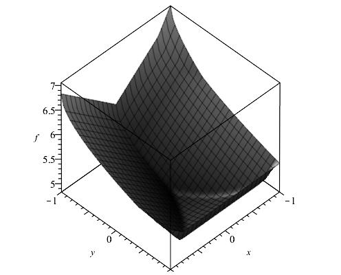
Figure 2: A Maple [20] snapshot. Left: Plot of ff with α=1\alpha=1. Right: Plot of f∗f^{*} with α=1\alpha=1.
Example 7.6

Let α≥0\alpha\geq 0. Define f:ℝ2→]−∞,+∞]f:\mathbb{R}^{2}\rightarrow\,\left]-\infty,+\infty\right] by

f⁡(x1,x2):={max⁡{α−x1,x2} if x1≥0,+∞ otherwise.f(x_{1},x_{2}):=\begin{cases}\max\{\alpha-\sqrt{x_{1}},x_{2}\}&\text{ if $x_{1}\geq 0$},\\ +\infty&\text{ otherwise.}\end{cases}

Then

∂f⁡(x1,x2)={(−1/2x1−1/2,0) if x1>0, and x2<α−x1,conv{(0,1),(−1/2x1−1/2,0)} if x1>0, and x2=α−x1,{(0,1)} if x1>0, and x2>α−x1,∅ if x1=0, and x2<α,ℝ−×{1} if x1=0, and x2≥α,∅ if x1<0.\partial f(x_{1},x_{2})=\begin{cases}(-1/2x_{1}^{-1/2},0)&\text{ if $x_{1}>0$, and $x_{2}<\alpha-\sqrt{x_{1}}$,}\\ \operatorname{conv}\{(0,1),(-1/2x_{1}^{-1/2},0)\}&\text{ if $x_{1}>0$, and $x_{2}=\alpha-\sqrt{x_{1}}$,}\\ \{(0,1)\}&\text{ if $x_{1}>0$, and $x_{2}>\alpha-\sqrt{x_{1}}$,}\\ \varnothing&\text{ if $x_{1}=0$, and $x_{2}<\alpha$,}\\ \mathbb{R}_{-}\times\{1\}&\text{ if $x_{1}=0$, and $x_{2}\geq\alpha$,}\\ \varnothing&\text{ if $x_{1}<0$.}\end{cases}

In particular, dom∂f={(x1,x2)∣x1≥0}∖{(0,x2)∣x2<α}\operatorname{dom}\partial f=\big\{{(x_{1},x_{2})}\mid{x_{1}\geq 0}\big\}\setminus\big\{{(0,x_{2})}\mid{x_{2}<\alpha}\big\} is neither open nor closed, but it is convex. The same holds for the range

ran∂f={(x1,x2)∣x1≤0,0≤x2≤1}∖{(0,x2)∣0≤x2<1}.\operatorname{ran}\partial f=\big\{{(x_{1},x_{2})}\mid{x_{1}\leq 0,0\leq x_{2}\leq 1}\big\}\setminus\big\{{(0,x_{2})}\mid{0\leq x_{2}<1}\big\}.

See Appendix A for its proof.

We are finally positioned to construct proper lower semicontinuous convex functions on ℝ2\mathbb{R}^{2} whose subdifferential domains are nearly polyhedral sets but nonconvex. Recall that C⊆ℝnC\subseteq\mathbb{R}^{n} is said to be polyhedral if it can be expressed as the intersection of a finite family closed half spaces or hyperplanes, i.e.,

C=(∩i=1m{x∈ℝn∣fi(x)≤0})⋂(∩j=1k{x∈ℝn∣fj(x)=0})C=\big(\cap_{i=1}^{m}\big\{{x\in\mathbb{R}^{n}}\mid{f_{i}(x)\leq 0}\big\}\big)\bigcap\big(\cap_{j=1}^{k}\big\{{x\in\mathbb{R}^{n}}\mid{f_{j}(x)=0}\big\}\big)

where each fif_{i} is affine.

Theorem 7.7

In ℝ2\mathbb{R}^{2}, every polyhedral set CC having a nonempty interior and having edges removed but keeping all its vertices is a domain of a subdifferential mapping of a proper lower semicontinuous convex function on ℝ2\mathbb{R}^{2}.

Proof. Each polyhedral set is closed and convex [26, Example 2.10]. Associated each edge [xi,xi+1][x_{i},x_{i+1}] of CC, one can find a closed half space Hi⊆ℝ2H_{i}\subseteq\mathbb{R}^{2} contains CC and has [xi,xi+1][x_{i},x_{i+1}] in its boundary. By using translation, rotation and dilation for the convex function in Example 7.5, we can get a lower semicontinuous convex function fi:ℝ2→]−∞,+∞]f_{i}:\mathbb{R}^{2}\rightarrow\,\left]-\infty,+\infty\right] such that dom∂fi=Hi∖]xi,xi+1[\operatorname{dom}\partial f_{i}=H_{i}\setminus]x_{i},x_{i+1}[. For each edge of the form emanating from xjx_{j} in the direction vjv_{j}: Rj={xj+τ​vj∣τ≥0}R_{j}=\big\{{x_{j}+\tau v_{j}}\mid{\tau\geq 0}\big\}, one can find a closed half space Hj⊆ℝ2H_{j}\subseteq\mathbb{R}^{2} containing CC and has RjR_{j} in its boundary. Again, by using translation, rotation, and dilation for the convex function in Example 7.6, we get a lower semicontinuous convex function fj:ℝ2→]−∞,+∞]f_{j}:\mathbb{R}^{2}\rightarrow\,\left]-\infty,+\infty\right] such that dom∂fj=Hj∖{xj+τvj∣τ>0}\operatorname{dom}\partial f_{j}=H_{j}\setminus\big\{{x_{j}+\tau v_{j}}\mid{\tau>0}\big\}. Define the lower semcontinuous convex function f:ℝ2→]−∞,+∞]f:\mathbb{R}^{2}\rightarrow\,\left]-\infty,+\infty\right] by

f:=ιcl⁡C+∑i∈Ifi+∑i∈Jfj.f:=\iota_{\operatorname{cl}{C}}+\sum_{i\in I}f_{i}+\sum_{i\in J}f_{j}.

As int⁡C≠∅\operatorname{int}C\neq\varnothing, by the subdifferential sum rule we have ∂f=∂ιcl⁡C+∑i∈I∂fi+∑i∈J∂fj.\partial f=\partial\iota_{\operatorname{cl}{C}}+\sum_{i\in I}\partial f_{i}+\sum_{i\in J}\partial f_{j}. The maximally monotone operator ∂f\partial f has dom∂f=C\operatorname{dom}\partial f=C. ■\quad\hfill\blacksquare

Immediately from Theorem 7.7, we see that each set in Figure 3 is the subdifferential domain of a proper lower semicontinuous convex function on ℝ2\mathbb{R}^{2}.

Refer to caption Refer to caption
Figure 3: A GeoGebra [17] snapshot. Nearly convex but not convex sets

As a concrete example, we have

Example 7.8

Suppose that f:ℝ2→]−∞,+∞]f:\mathbb{R}^{2}\to\,\left]-\infty,+\infty\right] is defined as f:=∑i∈Ifif:=\sum_{i\in I}f_{i}, where I:={1,2,3,4}I:=\{1,2,3,4\} and (∀i∈I)(\forall i\in I) fif_{i} are defined as

f1\displaystyle f_{1} :ℝ2→ℝ:(x,y)↦max⁡{2−12​(2+x−y),|12​(2+x+y)|},\displaystyle:\mathbb{R}^{2}\to\mathbb{R}:(x,y)\mapsto\max\left\{\sqrt{2}-\sqrt{\tfrac{1}{\sqrt{2}}(2+x-y)},\lvert\tfrac{1}{\sqrt{2}}(2+x+y)\rvert\right\}, (41)
f2\displaystyle f_{2} :ℝ2→ℝ:(x,y)↦max⁡{3−1+y,|x|},\displaystyle:\mathbb{R}^{2}\to\mathbb{R}:(x,y)\mapsto\max\left\{3-\sqrt{1+y},\lvert x\rvert\right\}, (42)
f3\displaystyle f_{3} :ℝ2→ℝ:(x,y)↦max⁡{1−1−y,|x|},\displaystyle:\mathbb{R}^{2}\to\mathbb{R}:(x,y)\mapsto\max\left\{1-\sqrt{1-y},\lvert x\rvert\right\}, (43)
f4\displaystyle f_{4} :ℝ2→ℝ:(x,y)↦max⁡{2−12​(2−x−y),|12​(−2+x−y)|}.\displaystyle:\mathbb{R}^{2}\to\mathbb{R}:(x,y)\mapsto\max\left\{\sqrt{2}-\sqrt{\tfrac{1}{\sqrt{2}}(2-x-y)},\lvert\tfrac{1}{\sqrt{2}}(-2+x-y)\rvert\right\}. (44)

Then ff is a proper, convex, lower semicontinuous function and

dom∂f=ran(∂f)−1=ran∂f∗\displaystyle\operatorname{dom}{\partial}f=\operatorname{ran}({\partial}f)^{-1}=\operatorname{ran}{\partial}f^{*}
={(x,y)||x|<3,|y|<1,2+x−y>0,2−x−y>0}∪{(1,1),(−1,1),(3,−1),(−3,−1)},\displaystyle=\left\{(x,y)~|~\lvert x\rvert<3,\lvert y\rvert<1,2+x-y>0,2-x-y>0\right\}\cup\left\{(1,1),(-1,1),(3,-1),(-3,-1)\right\},

as shown in Figure 4.

Refer to caption
(a) f⁡(ξ1,ξ2)f(\xi_{1},\xi_{2})
Refer to caption
(b) dom∂f\operatorname{dom}{\partial}f
Figure 4: The function ff and dom∂f\operatorname{dom}{\partial}f of Example 7.8.

Proof. Let

gα:ℝ2→ℝ:(x,y)↦{max⁡{α−x,|y|}, if ​x≥0;+∞,otherwise,g_{\alpha}:\mathbb{R}^{2}\to\mathbb{R}:(x,y)\mapsto\begin{cases}\max\left\{\alpha-\sqrt{x},\lvert y\rvert\right\},&\text{ if }x\geq 0;\\ +\infty,&\text{otherwise,}\end{cases}

and

Rθ=(cos⁡θ−sin⁡θsin⁡θcos⁡θ).R_{\theta}=\begin{pmatrix}\cos\theta&-\sin\theta\\ \sin\theta&\cos\theta\end{pmatrix}.

Then (∀(x,y)∈ℝ2)(\forall(x,y)\in\mathbb{R}^{2}) we have,

f1​(x,y)\displaystyle f_{1}(x,y) =g2​(Rπ/4​((x,y)−(−2,0))),\displaystyle=g_{\sqrt{2}}(R_{\pi/4}((x,y)-(-2,0))),
f2​(x,y)\displaystyle f_{2}(x,y) =g3(R−π/2((x,y)−(0,−1))),\displaystyle=g_{3}(R_{-\pi/2}((x,y)-(0,-1))),
f3​(x,y)\displaystyle f_{3}(x,y) =g1​(Rπ/2​((x,y)−(0,1))),\displaystyle=g_{1}(R_{\pi/2}((x,y)-(0,1))),
f4​(x,y)\displaystyle f_{4}(x,y) =g2​(R5​π/4​((x,y)−(2,0))).\displaystyle=g_{\sqrt{2}}(R_{5\pi/4}((x,y)-(2,0))).

As ∂f=∑i∈I∂fi{\partial}f=\sum_{i\in I}{\partial}f_{i}, using Example 7.5, and particularly (39), we see that

dom∂f=∩i∈Idom∂fi\displaystyle\operatorname{dom}{\partial}f=\cap_{i\in I}\operatorname{dom}{\partial}f_{i}
={(x,y)||x|<3,|y|<1,2+x−y>0,2−x−y>0}∪{(1,1),(−1,1),(3,−1),(−3,−1)}.\displaystyle=\left\{(x,y)~|~\lvert x\rvert<3,\lvert y\rvert<1,2+x-y>0,2-x-y>0\right\}\cup\left\{(1,1),(-1,1),(3,-1),(-3,-1)\right\}.

Using [4, Proposition 16.24] we have (∂f)−1=∂f∗({\partial}f)^{-1}={\partial}f^{*}, which completes the proof. ■\quad\hfill\blacksquare

We finish this section by remarking that each set in Figure 1 is a subdifferential domain of a proper lower semicontinuous convex function. For the first set, use f:=ιB⁡(0,1)+g1+g2f:=\iota_{B(0,1)}+g_{1}+g_{2} where each gig_{i} has dom∂gi\operatorname{dom}\partial g_{i} being an open convex set whose boundary consists of one dotted line part of the unit circle and two dotted rays tangent to the circle. For the second set, use f:=ιB⁡(0,1)+g1+g2f:=\iota_{B(0,1)}+g_{1}+g_{2} where each gig_{i} is obtained by rotation and translation of Rockafellar’s function, and dom∂gi\operatorname{dom}\partial g_{i} is a closed half space with an open line segment on its boundary removed.

8 Discussions and open problems

In this paper we systematically study nearly convex sets: criteria for near convexity; topological properties such as relative interior, interior, recession cone of nearly convex sets; formulas for the relative interiors and closures of nearly convex sets, which are linear image or inverse image of other nearly convex sets. Rockafellar provided the first convex function whose subdifferential domain is not convex. To build more examples, we compute the subdifferential and the Fenchel conjugate of an modified Rockafellar’s function. It turns out every polyhedral set in ℝ2\mathbb{R}^{2} with edges removed but keeping its vertices is a domain of the subdifferential mapping of a proper lower semicontinuous convex function.

Although we have constructed some proper lower semicontinuous convex functions whose subdifferential mappings have prescribed domain or ranges, the general problem is still unsolved. Let us note that

Theorem 8.1

Let C⊆ℝnC\subseteq\mathbb{R}^{n} (not necessarily convex). Then there exists a monotone operator (not necessarily maximal monotone) A:ℝn⇉ℝnA:\mathbb{R}^{n}\rightrightarrows\mathbb{R}^{n} such that ran⁡A=C\operatorname{ran}A=C.

Proof. Consider the projection operator PC:ℝn⇉ℝnP_{C}:\mathbb{R}^{n}\rightrightarrows\mathbb{R}^{n}. Then PCP_{C} is monotone because gra⁡PC⊆gra⁡Pcl⁡C\operatorname{gra}P_{C}\subseteq\operatorname{gra}P_{\operatorname{cl}{C}}, and Pcl⁡CP_{\operatorname{cl}{C}} is monotone by [26, Proposition 12.19]. Clearly ran⁡PC=C\operatorname{ran}P_{C}=C. ■\quad\hfill\blacksquare

According to [26, Theorem 12.20], a closed set C⊆ℝnC\subseteq\mathbb{R}^{n} is convex if and only if PCP_{C} is maximally monotone. Therefore, it is the maximality to force CC having more structural properties.

We finish the paper with three open questions:

  1. (i)

    Is every convex set a domain or range of a subdifferential mapping of a proper lower semicontinuous convex function (or a maximally monotone operator) in ℝn\mathbb{R}^{n} with n≥2n\geq 2?

  2. (ii)

    Is every nearly convex set a domain or range of a subdifferential mapping of a proper lower semicontinuous convex function (or a maximally monotone operator) in ℝn\mathbb{R}^{n} with n≥2n\geq 2?

  3. (iii)

    What is the intrinsic difference between the ranges of subdifferentials of proper lower semicontinuous convex functions and the ranges of maximally monotone operators?

Acknowledgments

Sarah Moffat was partially supported by the Natural Sciences and Engineering Research Council of Canada. Walaa Moursi was supported by NSERC grants of Drs. Heinz Bauschke and Warren Hare. Xianfu Wang was partially supported by the Natural Sciences and Engineering Research Council of Canada.

Appendix A

We shall need two facts. The first one is a structural characterization of ∂f\partial f when a convex function ff is lower semicontinuous, and ∇f\nabla f is not empty. (See also [26, Theorem 12.67] for the structure of maximally monotone operators.) The second one concerns the domain of the Fenchel conjugate of convex functions.

Fact 8.2

([24, Theorem 25.6]) Let ff be a closed proper convex function such that dom⁡f\operatorname{dom}f has a non-empty interior. Then

∂f⁡(x)=cl⁡(conv⁡S⁡(x))+K⁡(x),∀x,\partial f(x)=\operatorname{cl}(\operatorname{conv}S(x))+K(x),\quad\forall x,

where K⁡(x)K(x) is the normal cone to dom⁡f\operatorname{dom}f at xx (empty if x∉dom⁡fx\not\in\operatorname{dom}f) and S⁡(x)S(x) is the set of all limits of sequence of the form ∇f​(x1),∇f​(x2),…,\nabla f(x_{1}),\nabla f(x_{2}),\ldots, such that ff is differentiable at xix_{i}, and xix_{i} tends to xx.

Lemma 8.3

Assume that f:ℝn→]−∞,+∞]f:\mathbb{R}^{n}\rightarrow\,\left]-\infty,+\infty\right] is proper lower semicontinuous convex function. If ran∂f\operatorname{ran}\partial f is closed, then domf∗=ran∂f\operatorname{dom}f^{*}=\operatorname{ran}\partial f.

Proof. As ran∂f=dom∂f∗\operatorname{ran}\partial f=\operatorname{dom}\partial f^{*}, by the Bronsted-Rockafellar’s theorem [23, Theorem 3.17] or [4, Proposition 16.28], we obtain ran∂f⊆domf∗⊆cl(ran∂f).\operatorname{ran}\partial f\subseteq\operatorname{dom}f^{*}\subseteq\operatorname{cl}(\operatorname{ran}\partial f). Therefore, the result holds. ■\quad\hfill\blacksquare

I. Proof of Example 7.5

Proof. First, we calculate ∂f\partial f. We argue by cases:

  1. (i)

    α−ξ1>|ξ2|\alpha-\sqrt{\xi_{1}}>\lvert\xi_{2}\rvert, 0<ξ1<α20<\xi_{1}<\alpha^{2}: ∇f(ξ1,ξ2)={(−12ξ1−1/2,0)}\nabla f(\xi_{1},\xi_{2})=\left\{(-\tfrac{1}{2}{\xi_{1}}^{-1/2},0)\right\} because f⁡(ξ1,ξ2)=α−ξ11/2f(\xi_{1},\xi_{2})=\alpha-{\xi_{1}}^{1/2}.

  2. (ii)

    ξ1=0\xi_{1}=0, |ξ2|<α\lvert\xi_{2}\rvert<\alpha: ∂f⁡(0,ξ2)=∅{\partial}f(0,\xi_{2})=\varnothing. Indeed, by (i), lim(x1,x2)→(0,ξ2)∇f(x1,x2)=lim(x1,x2)→(0,ξ2)(−12x1−1/2,0)\lim_{(x_{1},x_{2})\rightarrow(0,\xi_{2})}\nabla f(x_{1},x_{2})=\lim_{(x_{1},x_{2})\rightarrow(0,\xi_{2})}(-\tfrac{1}{2}{x_{1}}^{-1/2},0) does not exists. Apply Fact 8.2.

  3. (iii)

    ξ1=0\xi_{1}=0, ξ2≥α\xi_{2}\geq\alpha: ∂f⁡(0,ξ2)=ℝ−×{1}{\partial}f(0,\xi_{2})=\mathbb{R}_{-}\times\left\{1\right\}. Note that Ndom⁡f​(0,ξ2)=ℝ−×{0}N_{\operatorname{dom}f}(0,\xi_{2})=\mathbb{R}_{-}\times\{0\}. When x2>α−x1x_{2}>\alpha-\sqrt{x_{1}}, α2>x1>0\alpha^{2}>x_{1}>0, we have f⁡(x1,x2)=x2f(x_{1},x_{2})=x_{2}, so

    lim(x1,x2)→(0,ξ2)∇f​(x1,x2)={(0,1)};\lim_{(x_{1},x_{2})\rightarrow(0,\xi_{2})}\nabla f(x_{1},x_{2})=\{(0,1)\};

    When α−x1>x2\alpha-\sqrt{x_{1}}>x_{2}, 0<x1<α20<x_{1}<\alpha^{2}, x2>0x_{2}>0, we have f⁡(x1,x2)=α−x11/2f(x_{1},x_{2})=\alpha-{x_{1}}^{1/2}, so

    lim(x1,x2)→(0,ξ2)∇f(x1,x2)=lim(x1,x2)→(0,ξ2)(−12x1−1/2,0)\lim_{(x_{1},x_{2})\rightarrow(0,\xi_{2})}\nabla f(x_{1},x_{2})=\lim_{(x_{1},x_{2})\rightarrow(0,\xi_{2})}(-\tfrac{1}{2}{x_{1}}^{-1/2},0)

    does not exist. Apply Fact 8.2 to obtain ∂f⁡(0,ξ2)\partial f(0,\xi_{2}).

  4. (iv)

    ξ1=0\xi_{1}=0, ξ2≤−α\xi_{2}\leq-\alpha: ∂f⁡(0,ξ2)=ℝ−×{−1}{\partial}f(0,\xi_{2})=\mathbb{R}_{-}\times\left\{-1\right\}. The arguments are similar to (iii).

  5. (v)

    ξ2>α−ξ1\xi_{2}>\alpha-\sqrt{\xi_{1}}, α2>ξ1>0\alpha^{2}>\xi_{1}>0: ∂f⁡(ξ1,ξ2)={(0,1)}\partial f(\xi_{1},\xi_{2})=\{(0,1)\} because f⁡(ξ1,ξ2)=ξ2f(\xi_{1},\xi_{2})=\xi_{2}.

  6. (vi)

    ξ2=α−ξ1\xi_{2}=\alpha-\sqrt{\xi_{1}}, α2>ξ1>0\alpha^{2}>\xi_{1}>0: Notice that f⁡(ξ1,ξ2)=max⁡{f1​(ξ1,ξ2),f2​(ξ1,ξ2)}f(\xi_{1},\xi_{2})=\max\left\{f_{1}(\xi_{1},\xi_{2}),f_{2}(\xi_{1},\xi_{2})\right\}, where f1​(ξ1,ξ2)=α−ξ1f_{1}(\xi_{1},\xi_{2})=\alpha-\sqrt{\xi_{1}} and f2​(ξ1,ξ2)=ξ2f_{2}(\xi_{1},\xi_{2})=\xi_{2}. When |ξ2|=α−ξ1\lvert\xi_{2}\rvert=\alpha-\sqrt{\xi_{1}}, ξ1>0\xi_{1}>0, and ξ2>0\xi_{2}>0, we have f1​(ξ1,ξ2)=f2​(ξ1,ξ2)f_{1}(\xi_{1},\xi_{2})=f_{2}(\xi_{1},\xi_{2}), hence it follows from [26, Theorem 10.31] that

    ∂f⁡(ξ1,ξ2)=conv⁡{∇f1​(ξ1,ξ2),∇f1​(ξ1,ξ2)}=conv⁡{(−12​ξ1−12,0),(0,1)}.{\partial}{f(\xi_{1},\xi_{2})}=\operatorname{conv}\left\{\nabla f_{1}(\xi_{1},\xi_{2}),\nabla f_{1}(\xi_{1},\xi_{2})\right\}=\operatorname{conv}\left\{(-\tfrac{1}{2}{\xi_{1}}^{-\tfrac{1}{2}},0),(0,1)\right\}.
  7. (vii)

    −ξ2=α−ξ1-\xi_{2}=\alpha-\sqrt{\xi_{1}}, α2>ξ1>0\alpha^{2}>\xi_{1}>0: The proof is similar to the previous case with f⁡(ξ1,ξ2)=max⁡{f1​(ξ1,ξ2),f2​(ξ1,ξ2)}f(\xi_{1},\xi_{2})=\max\left\{f_{1}(\xi_{1},\xi_{2}),f_{2}(\xi_{1},\xi_{2})\right\}, where f1​(ξ1,ξ2)=α−ξ1,f_{1}(\xi_{1},\xi_{2})=\alpha-\sqrt{\xi_{1}}, and f2​(ξ1,ξ2)=−ξ2f_{2}(\xi_{1},\xi_{2})=-\xi_{2}, thus

    ∂f(ξ1,ξ2)=conv{(−12ξ1−1/2,0),(0,−1)}.{\partial}{f(\xi_{1},\xi_{2})}=\operatorname{conv}\left\{(-\tfrac{1}{2}{\xi_{1}}^{-{1}/{2}},0),(0,-1)\right\}.
  8. (viii)

    ξ1=α2\xi_{1}=\alpha^{2}, ξ2=0\xi_{2}=0: We have f⁡(ξ1,ξ2)=max⁡{f1​(ξ1,ξ2),f2​(ξ1,ξ2),f3​(ξ1,ξ2)}f(\xi_{1},\xi_{2})=\max\left\{f_{1}(\xi_{1},\xi_{2}),f_{2}(\xi_{1},\xi_{2}),f_{3}(\xi_{1},\xi_{2})\right\}, where f1​(ξ1,ξ2)=α−ξ1,f_{1}(\xi_{1},\xi_{2})=\alpha-\sqrt{\xi_{1}}, f2​(ξ1,ξ2)=ξ2f_{2}(\xi_{1},\xi_{2})=\xi_{2} and f3​(ξ1,ξ2)=−ξ2f_{3}(\xi_{1},\xi_{2})=-\xi_{2}, thus

    ∂f⁡(ξ1,ξ2)=conv⁡{(−12​α,0),(0,1),(0,−1)}.{\partial}{f(\xi_{1},\xi_{2})}=\operatorname{conv}\left\{(-\tfrac{1}{2\alpha},0),(0,1),(0,-1)\right\}.
  9. (ix)

    When ξ1>α2\xi_{1}>\alpha^{2}, f⁡(ξ1,ξ2)=|ξ2|=max⁡{ξ2,−ξ2}f(\xi_{1},\xi_{2})=\lvert\xi_{2}\rvert=\max\left\{\xi_{2},-\xi_{2}\right\}. If ξ2>0\xi_{2}>0, then f⁡(ξ1,ξ2)=ξ2f(\xi_{1},\xi_{2})=\xi_{2}, so ∂f⁡(ξ1,ξ2)={(0,1)}{\partial}f(\xi_{1},\xi_{2})=\left\{(0,1)\right\}. If ξ2<0\xi_{2}<0, then f⁡(ξ1,ξ2)=−ξ2f(\xi_{1},\xi_{2})=-\xi_{2}, so ∂f⁡(ξ1,ξ2)={(0,−1)}{\partial}f(\xi_{1},\xi_{2})=\left\{(0,-1)\right\}. If ξ2=0\xi_{2}=0, then ∂f⁡(ξ1,0)=conv⁡{(0,1),(0,−1)}={0}×[−1,1]\partial f(\xi_{1},0)=\operatorname{conv}\{(0,1),(0,-1)\}=\{0\}\times[-1,1].

Next, we calculate the Fenchel conjugate of ff.

In view of (38), ran∂f\operatorname{ran}\partial f is closed, so domf∗=ran∂f\operatorname{dom}f^{*}=\operatorname{ran}\partial f by Lemma 8.3. Recall that

f∗​(x1∗,x2∗)=x1​x1∗+x2​x2∗−f⁡(x1,x2)f^{*}(x_{1}^{*},x_{2}^{*})=x_{1}x_{1}^{*}+x_{2}x_{2}^{*}-f(x_{1},x_{2}) (45)

We proceed by cases using (37).

  1. (i)

    x1∗≤0x_{1}^{*}\leq 0 and x2∗=1x_{2}^{*}=1: In this case x1=0x_{1}=0 and |x2|=x2≥α\lvert x_{2}\rvert=x_{2}\geq\alpha, hence f⁡(x1,x2)=x2f(x_{1},x_{2})=x_{2}. Therefore (45) implies that f∗​(x1∗,x2∗)=x2−x2=0f^{*}(x_{1}^{*},x_{2}^{*})=x_{2}-x_{2}=0.

  2. (ii)

    x1∗≤0x_{1}^{*}\leq 0 and x2∗=−1x_{2}^{*}=-1: In this case x1=0x_{1}=0 and |x2|=−x2≥α\lvert x_{2}\rvert=-x_{2}\geq\alpha, hence f⁡(x1,x2)=−x2f(x_{1},x_{2})=-x_{2}. Therefore (45) implies that f∗​(x1∗,x2∗)=−x2+x2=0f^{*}(x_{1}^{*},x_{2}^{*})=-x_{2}+x_{2}=0.

  3. (iii)

    −1/(2α)≤x1∗≤0-1/(2\alpha)\leq x_{1}^{*}\leq 0 and |x2∗|≤1+2​α​x1∗|x_{2}^{*}|\leq 1+2\alpha x_{1}^{*}: In this case, this is exactly the region given by the set conv⁡{(−12​α,0),(0,1),(0,−1)}=∂f⁡(α2,0)\operatorname{conv}\left\{(-\tfrac{1}{2\alpha},0),(0,1),(0,-1)\right\}=\partial f(\alpha^{2},0). Hence, by (37) we have (x1∗,x2∗)∈∂f⁡(α2,0)(x_{1}^{*},x_{2}^{*})\in\partial f(\alpha^{2},0) so that x1=α2x_{1}=\alpha^{2}, x2=0x_{2}=0 and f⁡(x1,x2)=0f(x_{1},x_{2})=0. Therefore,

    f∗​(x1∗,x2∗)\displaystyle f^{*}(x_{1}^{*},x_{2}^{*}) =x1​x1∗+x2​x2∗−f⁡(x1,x2)\displaystyle=x_{1}x_{1}^{*}+x_{2}x_{2}^{*}-f(x_{1},x_{2})
    =α2⋅x1∗+0⋅x2∗−0=α2​x1∗.\displaystyle=\alpha^{2}\cdot x_{1}^{*}+0\cdot x_{2}^{*}-0=\alpha^{2}x_{1}^{*}. (46)
  4. (iv)

    x1∗<0x_{1}^{*}<0 and max⁡{0,1+2​α​x1∗}≤x2∗<1\max\{0,1+2\alpha x_{1}^{*}\}\leq x_{2}^{*}<1: In this case, this is the region given by

    ⋃{conv{(−1/2x1−1/2,0),(0,1)}:0<x1<α2,x2=α−x11/2}∖{(0,1)}.\bigcup\left\{\operatorname{conv}\{(-1/2x_{1}^{-1/2},0),(0,1)\}:0<x_{1}<\alpha^{2},x_{2}=\alpha-x_{1}^{1/2}\right\}\setminus\{(0,1)\}.

    Then each (x1∗,x2∗)∈conv⁡{(−12​x1,0),(0,1)}(x_{1}^{*},x_{2}^{*})\in\operatorname{conv}\left\{(-\tfrac{1}{2\sqrt{x_{1}}},0),(0,1)\right\} for some (x1,x2)(x_{1},x_{2}) satisfying 0<x1<α2,x2=α−x11/20<x_{1}<\alpha^{2},x_{2}=\alpha-x_{1}^{1/2}. Thus, there exists λ∈]0,1]\lambda\in\left]0,1\right] such that x1∗=−λ2​x1x_{1}^{*}=-\tfrac{\lambda}{2\sqrt{x_{1}}} and x2∗=1−λx_{2}^{*}=1-\lambda. Therefore we have 1x1=−2λ​x1∗=−21−x2∗​x1∗\tfrac{1}{\sqrt{x_{1}}}=-\tfrac{2}{\lambda}x_{1}^{*}=-\tfrac{2}{1-x_{2}^{*}}x_{1}^{*}, x1=−1−x2∗2​x1∗\sqrt{x_{1}}=-\tfrac{1-x_{2}^{*}}{2x_{1}^{*}}, x2=α−x1=α+1−x2∗2​x1∗x_{2}=\alpha-\sqrt{x_{1}}=\alpha+\tfrac{1-x_{2}^{*}}{2x_{1}^{*}}, and f⁡(x1,x2)=α−x1=x2f(x_{1},x_{2})=\alpha-\sqrt{x_{1}}=x_{2}. Now (45) implies that

    f∗​(x1∗,x2∗)\displaystyle f^{*}(x_{1}^{*},x_{2}^{*}) =x1​x1∗+x2​x2∗−f⁡(x1,x2)\displaystyle=x_{1}x_{1}^{*}+x_{2}x_{2}^{*}-f(x_{1},x_{2})
    =(1−x2∗)24​x1∗2​x1∗+(α+1−x2∗2​x1∗)​x2∗−(α+1−x2∗2​x1∗)\displaystyle=\tfrac{(1-x_{2}^{*})^{2}}{4{x_{1}^{*}}^{2}}x_{1}^{*}+(\alpha+\tfrac{1-x_{2}^{*}}{2x_{1}^{*}})x_{2}^{*}-(\alpha+\tfrac{1-x_{2}^{*}}{2x_{1}^{*}})
    =(1−x2∗)24​x1∗+(α+1−x2∗2​x1∗)​(x2∗−1)=(1−x2∗)24​x1∗−(1−x2∗)22​x1∗−α⁡(1−x2∗)\displaystyle=\tfrac{(1-x_{2}^{*})^{2}}{4{x_{1}^{*}}}+(\alpha+\tfrac{1-x_{2}^{*}}{2x_{1}^{*}})(x_{2}^{*}-1)=\tfrac{(1-x_{2}^{*})^{2}}{4{x_{1}^{*}}}-\tfrac{(1-x_{2}^{*})^{2}}{2{x_{1}^{*}}}-\alpha(1-x_{2}^{*})
    =−(1−x2∗)24​x1∗−α⁡(1−x2∗).\displaystyle=-\tfrac{(1-x_{2}^{*})^{2}}{4{x_{1}^{*}}}-\alpha(1-x_{2}^{*}).
  5. (v)

    x1∗<0x_{1}^{*}<0 and −1<x2∗≤min⁡{0,−(1+2​α​x1∗)}-1<x_{2}^{*}\leq\min\{0,-(1+2\alpha x_{1}^{*})\}: In this case, this is the region given by

    ⋃{conv{(−1/2x1−1/2,0),(0,−1)}:0<x1<α2,−x2=α−x11/2}∖{(0,−1)}.\bigcup\left\{\operatorname{conv}\{(-1/2x_{1}^{-1/2},0),(0,-1)\}:0<x_{1}<\alpha^{2},-x_{2}=\alpha-x_{1}^{1/2}\right\}\setminus\{(0,-1)\}.

    Then each (x1∗,x2∗)∈conv⁡{(−12​x1,0),(0,−1)}(x_{1}^{*},x_{2}^{*})\in\operatorname{conv}\left\{(-\tfrac{1}{2\sqrt{x_{1}}},0),(0,-1)\right\} for some (x1,x2)(x_{1},x_{2}) satisfying 0<x1<α2,−x2=α−x11/20<x_{1}<\alpha^{2},-x_{2}=\alpha-x_{1}^{1/2}. As before, let λ∈]0,1]\lambda\in\left]0,1\right]. Then x1∗=−λ2​x1x_{1}^{*}=-\tfrac{\lambda}{2\sqrt{x_{1}}} and x2∗=−(1−λ)=λ−1x_{2}^{*}=-(1-\lambda)=\lambda-1. Therefore we have 1x1=−2λ​x1∗=−21+x2∗​x1∗\tfrac{1}{\sqrt{x_{1}}}=-\tfrac{2}{\lambda}x_{1}^{*}=-\tfrac{2}{1+x_{2}^{*}}x_{1}^{*}, x1=−1+x2∗2​x1∗\sqrt{x_{1}}=-\tfrac{1+x_{2}^{*}}{2x_{1}^{*}}, x2=−(α−x1)=−α−1+x2∗2​x1∗x_{2}=-(\alpha-\sqrt{x_{1}})=-\alpha-\tfrac{1+x_{2}^{*}}{2x_{1}^{*}}, and f⁡(x1,x2)=α−x1=−x2f(x_{1},x_{2})=\alpha-\sqrt{x_{1}}=-x_{2}. Now (45) implies that

    f∗​(x1∗,x2∗)\displaystyle f^{*}(x_{1}^{*},x_{2}^{*}) =x1​x1∗+x2​x2∗−f⁡(x1,x2)\displaystyle=x_{1}x_{1}^{*}+x_{2}x_{2}^{*}-f(x_{1},x_{2})
    =(1+x2∗)24​x1∗2​x1∗−(α+1+x2∗2​x1∗)​x2∗−(α+1+x2∗2​x1∗)\displaystyle=\tfrac{(1+x_{2}^{*})^{2}}{4{x_{1}^{*}}^{2}}x_{1}^{*}-(\alpha+\tfrac{1+x_{2}^{*}}{2x_{1}^{*}})x_{2}^{*}-(\alpha+\tfrac{1+x_{2}^{*}}{2x_{1}^{*}})
    =(1+x2∗)24​x1∗−(α+1+x2∗2​x1∗)​(x2∗+1)=(1+x2∗)24​x1∗−(1+x2∗)22​x1∗−α⁡(1+x2∗)\displaystyle=\tfrac{(1+x_{2}^{*})^{2}}{4{x_{1}^{*}}}-(\alpha+\tfrac{1+x_{2}^{*}}{2x_{1}^{*}})(x_{2}^{*}+1)=\tfrac{(1+x_{2}^{*})^{2}}{4{x_{1}^{*}}}-\tfrac{(1+x_{2}^{*})^{2}}{2{x_{1}^{*}}}-\alpha(1+x_{2}^{*})
    =−(1+x2∗)24​x1∗−α⁡(1+x2∗)=−(1−|x2∗|)24​x1∗−α⁡(1−|x2∗|).\displaystyle=-\tfrac{(1+x_{2}^{*})^{2}}{4{x_{1}^{*}}}-\alpha(1+x_{2}^{*})=-\tfrac{(1-\lvert x_{2}^{*}\rvert)^{2}}{4{x_{1}^{*}}}-\alpha(1-\lvert x_{2}^{*}\rvert). (47)

    (i)-(v) together finish the computation of f∗f^{*}.

Altogether, the proof is complete. ■\quad\hfill\blacksquare

II. Proof of Example 7.6

Proof. We argue by cases.

Case 1: x2<α−x1x_{2}<\alpha-\sqrt{x_{1}} and x1≥0x_{1}\geq 0. We have f⁡(x1,x2):=α−x1f(x_{1},x_{2}):=\alpha-\sqrt{x_{1}}. When x1>0x_{1}>0, f⁡(x1,x2)=α−x1f(x_{1},x_{2})=\alpha-\sqrt{x_{1}} so ∂f(x1,x2)=(−1/2x1−1/2,0)\partial f(x_{1},x_{2})=(-1/2x_{1}^{-1/2},0); When x1=0x_{1}=0 and x2<αx_{2}<\alpha, f⁡(0,x2)=αf(0,x_{2})=\alpha, f⁡(x1,x2)=α−x1f(x_{1},x_{2})=\alpha-\sqrt{x_{1}} when x1>0x_{1}>0, so ∂f⁡(0,x2)=∅\partial f(0,x_{2})=\varnothing.

Case 2: x2>α−x1x_{2}>\alpha-\sqrt{x_{1}} and x1≥0x_{1}\geq 0. When x1>0x_{1}>0, f⁡(x1,x2)=x2f(x_{1},x_{2})=x_{2}, ∂f⁡(x1,x2)={(0,1)}\partial f(x_{1},x_{2})=\{(0,1)\}; When x1=0x_{1}=0, ∂f⁡(0,x2)=(0,1)+ℝ−×{0}\partial f(0,x_{2})=(0,1)+\mathbb{R}_{-}\times\{0\}.

Case 3: x2=α−x1x_{2}=\alpha-\sqrt{x_{1}}. When x1>0x_{1}>0, ∂f(x1,x2)=conv{(0,1),(−1/2x1−1/2,0)}\partial f(x_{1},x_{2})=\operatorname{conv}\{(0,1),(-1/2x_{1}^{-1/2},0)\}; When x1=0,x2=αx_{1}=0,x_{2}=\alpha, ∂f⁡(0,α)=(0,1)+ℝ−×{0}\partial f(0,\alpha)=(0,1)+\mathbb{R}_{-}\times\{0\}. ■\quad\hfill\blacksquare

References

  • [1] S. Bartz, H.H. Bauschke, J.M. Borwein, S. Reich, and X. Wang, “ Fitzpatrick functions, cyclic monotonicity and Rockafellar’s antiderivative,” Nonlinear Anal. 66, pp. 1198–1223, 2007.
  • [2] H.H. Bauschke, J.M. Borwein and X. Wang, “Fitzpatrick functions and continuous linear monotone operators,” SIAM J. Optim. 18, pp. 789–809, 2007.
  • [3] H.H. Bauschke, X. Wang and L. Yao, “On paramonotone monotone operators and rectangular monotone operators,” Optimization, pp. 1–18, 2012.
  • [4] H.H. Bauschke and P.L. Combettes, Convex Analysis and Monotone Operator Theory in Hilbert Spaces, Springer, 2011.
  • [5] H.H. Bauschke, S. Moffat and X. Wang, “Firmly nonexpansive mappings and maximally monotone operators: correspondence and duality,” Set-Valued Var. Anal. 20, pp. 131–153, 2012.
  • [6] H.H. Bauschke, S.M. Moffat, and X. Wang, “Near equality, near convexity, sums of maximally monotone operators, and averages of firmly nonexpansive mappings,” Mathematical Programming 139, pp. 55–70, 2013.
  • [7] Sedi Bartz, H.H. Bauschke, S.M. Moffat, and X. Wang, “The resolvent average of monotone operators: dominant and recessive properties,” http://arxiv.org/pdf/1505.02718.pdf
  • [8] J.F. Bonnans and A. Shapiro, Perturbation Analysis of Optimization Problems, Springer Series in Operations Research, Springer-Verlag, 2000.
  • [9] J.M. Borwein and A.S. Lewis, Convex Analysis and Nonlinear Optimization, second edition, Springer, New York, 2006.
  • [10] J.M. Borwein and Q. Zhu, Techniques of Variational Analysis, Springer-Verlag, New York, 2005.
  • [11] R.I. Boţ, S.M. Grad, and G. Wanka, “Almost convex functions: conjugacy and duality,” Lecture Notes in Economics and Mathematical Systems 583, pp. 101–114, 2006.
  • [12] R.I. Boţ, S.M. Grad, and G. Wanka, “Fenchel’s duality theorem for nearly convex functions,” J. Optim. Theory Appl. 132, pp. 509–515, 2007.
  • [13] R.I. Boţ, G. Kassay, G. Wanka, “Duality for almost convex optimization problema via the perturbation approach,” J. Glob. Optim. 42, pp. 385–399, 2008.
  • [14] H. Brezis, A. Haraux, Image d’une Somme d’opérateurs Monotones et Applications, Israel J. Math. 23, pp. 165–186, 1976.
  • [15] M. Fabian, P. Habala, P. Hájek, V. Montesinos Santalucía, J. Pelant, and V. Zizler, Functional Analysis and Infinite-dimensional Geometry, CMS Books in Mathematics/Ouvrages de Mathématiques de la SMC, 8. Springer-Verlag, New York, 2001.
  • [16] J.B.G. Frenk, G. Kassay, “Lagrangian duality and cone convexlike functions,” J. Optim. Theor. Appl. 132(3), pp. 207–222, 2007.
  • [17] http://www.geogebra.org/.
  • [18] N. Hadjisavvas, S. Komlósi, and S. Schaible, “Handbook of generalized convexity and generalized monotonicity, nonconvex optimization and its applications,” Springer-Verlag, New York, 2005.
  • [19] R. John, “Uses of generalized convexity and generalized monotonicity in economics,” In [18], pp. 619–666.
  • [20] http://www.maplesoft.com/.
  • [21] J.E. Martinez-Legaz, “Generalized convex duality and its economic applications,” In [18], pp. 237–292.
  • [22] G.J. Minty, “On the maximal domain of a ”monotone” function,” Michigan Math. J. 8, pp. 135–137, 1961.
  • [23] R.R. Phelps, Convex Functions, Monotone Operators and Differentiability, 2nd Edition, Springer-Verlag, 1993.
  • [24] R.T. Rockafellar, Convex Analysis, Princeton University Press, 1970.
  • [25] R.T. Rockafellar, “On the virtual convexity of the domain and range of a nonlinear maximal monotone operator,” Math. Ann. 185, pp. 81–90, 1970.
  • [26] R.T. Rockafellar and R. J-B Wets, Variational Analysis, Springer-Verlag, corrected 3rd printing, 2009.
  • [27] S. Simons, From Hahn-Banach to Monotonicity, Springer-Verlag, 2008.
  • [28] C. Zălinescu, Convex Analysis in General Vector Spaces, World Scientific Publishing, 2002.