Computation of Linear Comparison Equations for Stability Analysis of Interconnected Systems

Let us consider the dynamical system

with an equilibrium at the origin²² 2 Note that this is not a restrictive assumption, since by shifting of state variables, the origin can always be made an equilibrium point., and $f:\mathbb{R}^{n}\rightarrow\mathbb{R}^{n}$ is locally Lipschitz. The important notions of stability are:

The Lyapunov stability theorem [1, 21], also called Lyapunov’s first or direct method, presents a sufficient condition of stability through the construction of a certain positive definite function.

Here $\dot{\tilde{V}}(x)=\nabla{\tilde{V}}^{T}f(x)$. When there exists such a function $\tilde{V}\left(x\right)$, the region of attraction (ROA) of the stable equilibrium point at origin can be (conservatively) estimated as

The Lyapunov function can be scaled by $\gamma^{max}$, so that,

Henceforth, for simplicity, we would assume, without any serious loss of generality, that the ROA is estimated to be sub-level set of ${V}(x)=1$.

Relatively recent studies have shown that sum-of-squares based optimization techniques can be utilized in finding Lyapunov functions by restricting the search space to sum-of-square polynomials [6, 22, 23, 7]. Let us denote by $\mathbb{R}\left[x\right]$ the set of all polynomials in $x\in\mathbb{R}^{n}$. Then,

Checking if $p\in\mathbb{R}[x]$ is an SOS is a semi-definite problem which can be solved with a MATLAB${}^{\text{\textregistered}}$ toolbox SOSTOOLS [3, 4] along with a semidefinite programming solver such as SeDuMi [5]. SOS technique can be used to search for polynomial Lyapunov functions, by translating (2) to equivalent SOS conditions [3, 24, 6, 25, 26, 4, 27]. An important result from algebraic geometry called Putinar’s Positivstellensatz theorem [28, 29] helps in translating the SOS conditions into SOS feasibility problems. Then the Putinar’s Positivestellensatz theorem⁴⁴ 4 For other versions of the Positivstellensatz theorem please refer to [29]. states,

Often for the $u_{i},\,\forall i,$ used in this work, the existence of $u(x)$ in (2) would be guaranteed [29].

Before finishing this section, let us take a look at a nice result on the ordinary differential equations which helps form the framework of stability analysis of inter-connected systems via vector Lyapunov functions. Noting that all the elements of the vector $e^{At},~t\geq 0$, where $A=\left[a_{ij}\right]\in\mathbb{R}^{m\times m}$, are non-negative if and only if $a_{ij}\geq 0,i\neq j$, the authors in [16, 17] proposed the following result:

This result will henceforth be referred to as the ‘linear comparison principle’ and the differential equation in (9) as the ‘comparison equation’.

The dynamical system in (1) can be expressed in the form of $m$ ($\geq 2$) interacting, and asymptotically stable subsystems

Here $x_{i}$ represents the states that belong to the $i$-th subsystem $\mathcal{S}_{i}$, $f_{i}\in\mathbb{R}[x_{i}]^{n_{i}}$ denotes the isolated subsystem dynamics, and $g_{i}\in\mathbb{R}[x]^{n_{i}}$ represents the neighbor interactions.

Let us assume that the interactions can be expressed as

where $g_{ij}\in\mathbb{R}[x_{i},x_{j}]^{n_{i}}$ quantifies how subsystem $\mathcal{S}_{j}$ affects the dynamics of subsystem $\mathcal{S}_{i}$. Note that (11) is not a very restrictive assumption, since given the choice of states $x_{i}$ of the subsystem $\mathcal{S}_{i}$, the rest of the subsystems can always be chosen in a way such that (11) holds. We denote by

the set of indices of the subsystems in the neighborhood of $\mathcal{S}_{i}$ (including the subsystem itself) and the states that belong to this neighborhood, respectively.

The next step is to characterize the stability properties of the isolated subsystems

by computing a polynomial Lyapunov function $V_{i}\in\mathbb{R}\left[x_{i}\right]$ for each $i$, and the corresponding estimate of the ROA as in (5). An SOS based expanding interior algorithm, [6, 7], is used to iteratively enlarge the estimate of the ROA by finding a ‘better’ Lyapunov function at each step of the algorithm. At the completion of this iterative algorithm, the stability of each isolated subsystem (assuming no interaction) is quantified by its Lyapunov function $V_{i}\in\mathbb{R}[x_{i}]$, with a final estimate of the domain of attraction given by

Let us define the domain

which could be interpreted as the ROA of the ‘free’ interconnected system (10), in absence of the all the interactions. The disturbances coming from the neighbors can be expressed by the subsystem Lyapunov function level-sets. While the equilibrium at origin corresponds to the level sets $V_{i}(0)=0,\forall i$, any disturbance (or initial condition) away from this equilibrium would result in positive level-sets $V_{i}(x_{i}(0))=\gamma_{i}^{0}\in\left(0,1\right]$ for some or all of the subsystems.

A necessary and sufficient condition of asymptotic stability (Definition 1) can then be translated into the condition

where $x_{i}(t),~t>0$, are solutions of the coupled dynamics in (10). Even though (15) reduces the dimensionality of the problem, it still remains a generally non-trivial problem. An attractive, and scalable, alternative approach is to construct a vector Lyapunov function $V:\mathbb{R}^{n}\rightarrow\mathbb{R}^{m}$

and use a comparison equation to certify if the condition (15) holds. Restricting our focus to the linear comparison principle (Lemma 1), the aim is to seek an $A=[a_{ij}]\in\mathbb{R}^{m\times m}$ and a domain $\mathcal{D}\subset\mathcal{R}^{0}$, such that

If there exist a ‘comparison matrix’ $A=[a_{ij}]$ and $\mathcal{D}\subset\mathcal{R}^{0}$ satisfying (17), then any $x(0)\in\mathcal{D}$ would guarantee exponentially convergence of $V(x(t))$ to the origin (Lemma 1),

which also translates into exponential convergence of the states themselves [10]. Note that, $\mathcal{D}\subset\mathcal{R}^{0}$, if exists, presents an estimate of the ROA of the full interconnected system.

In [10, 11, 13, 19], and related works, authors laid out a formulation of the linear comparison equation using certain conditions on the Lyapunov functions and the neighbor interactions. It was observed that if there exists a set of Lyapunov functions, $v_{i}:\mathbb{R}^{n_{i}}\rightarrow\mathbb{R}\,,~\forall\,i=1,2,\dots,m,$ satisfying the following conditions

and if the interaction terms in (11) satisfy

then the following comparison equation can be formed,

If the ‘comparison matrix’ $\tilde{A}=[\tilde{a}_{ij}]$ is Hurwitz, then any invariant domain $\mathcal{R}\subseteq\mathcal{D}$ provides an estimate of a region of exponential stability of the full system [11, 19].

While this approach provides very useful analytical insights into the construction of the comparison matrix $\tilde{A}=[\tilde{a}_{ij}]$, it has certain computational issues. This requires finding the bounds in (19) and (20), and also the Lyapunov functions $v_{i},\,\forall\,i,$ that satisfy those. Clearly the polynomial Lyapunov functions, $V_{i}\,\forall\,i,$ cannot satisfy the linear bounds in (19).

Assuming that the polynomial Lyapunov functions, $V_{i}\,\forall\,i$, we found using the expanding interior algorithm (Sec. III-A) are quadratic, we can define $v_{i}:=\sqrt{V_{i}}\,,\,\forall\,i$, which would satisfy the conditions in (19) [11, 19]. In such a case, one needs to find the following bounds,

for some positive scalars ${\eta}_{i1},{\eta}_{i2},{\eta}_{i3},{\zeta}_{ij}$. Then using simple algebra the bounds in (19) and (20) can be obtained as

Thus the computation of each element of the comparison matrix $\tilde{A}$ in (21) requires multiple optimization steps.

We may also note that some of the bounds in (19) and (20), while convenient for analytical insights, need not be optimal for computing a Hurwitz comparison matrix. For example, in (20), $\left\|\nabla v_{i}^{T}g_{ij}\right\|_{2}$ is function of both $x_{i}$ and $x_{j}$ but is bounded by using only the norm on $x_{j}$.

We propose to use SOS methods to directly compute the comparison equation in (17), in a decentralized way by calculating each row of $A=[a_{ij}]$ directly at each subsystem level. Note that, in (17), we will be using quadratic (or, in general, polynomial) Lyapunov functions which do not satisfy the bounds (19)-(20). But we may observe that,

It will be useful to note here that, an application of Gershgorin’s Circle theorem [31] says that if a matrix with negative diagonal elements is strictly diagonally dominant⁶⁶ 6 $A=[a_{ij}]$ is strictly diagonally dominant if $\sum_{j\neq i}\left|a_{ij}\right|<\left|a_{ii}\right|,\forall i$. then the matrix is Hurwitz. We are now in a position to outline the SOS based procedure to directly compute the matrix $A=[a_{ij}]$ in the comparison equation (17).

In this work, we are interested in $\mathcal{D}_{i}\,,\forall\,i$, of the form,

Note that we exclude the boundary of the isolated subsystem ROA, $\gamma_{i}^{0}=1\,\forall\,i$, for reasons explained later. The comparison equation in (17a) can then be translated into

since we know that $a_{ij}=0~\forall j\notin\mathcal{N}_{i}$. Using the Positivstellensatz theorem (Theorem 2), with $u_{i}:=\left(\gamma_{i}^{0}-V_{i}(x_{i})\right)$ and $\mathcal{K}=\mathcal{D}$, we can cast (25) into an SOS feasibility problem,

where $\bar{x}_{i}$ was defined in (12). The goal is to find the ‘optimal’ scalars $a_{ij}\,\forall i,j\in\mathcal{N}_{i}$ satisfying (26) so as to obtain the tightest possible bound in (17a). We can thus formulate the following SOS optimization problem,

This simple SOS formulation helps us find the comparison equation (17) in a decentralized way, by computing each row of the comparison matrix $A=[a_{ij}]$ in a single optimization problem at each subsystem level. The optimization problem can be easily implemented on a parallel platform, with the complexity of the problem essentially dependent on the size of the largest neighborhood $\mathcal{N}_{i}$.

Further note that, if the minimal values of all the row-sums in (27) are negative, then the matrix $A=[a_{ij}]$ thus found is a strictly diagonally dominant with negative diagonal entries, and hence, Hurwitz [31]. However, if $\sum_{j=1}^{m}a_{ij}\geq 0$ for any $i$, then the eigenvalues of $A=[a_{ij}]$ need to be computed.

Finally a note on invariance of the domain $\mathcal{D}$, which along with the presence of Hurwitz $A=[a_{ij}]$ guarantees that $\mathcal{D}$ is a domain of exponential stability, as noted in (17). According to [11], an estimate of the ROA can be given by

Then it is easy to see that,

We consider a network of nine Van der Pol ‘oscillators’ [20], with parameters of each oscillator chosen to make them individually stable. Each Van der Pol oscillator constitutes a subsystem, with the interconnections shown below

The dynamics of each oscillator, in presence of the neighbor interactions, is given by

where $\mu_{j}\,,\,\forall j$, are chosen randomly from $\left(-3\,,\,-1\right)$ and the interaction coefficients $\beta_{jk}\,,\,\forall j,\forall k\!\!\in\!\!\mathcal{N}_{j}\backslash\left\{j\right\}$, are chosen randomly from $\left(-0.4\,,\,0.4\right)$.

Using the expanding interior algorithm, we find estimates of the ROAs of the isolated, or ‘free’, subsystems via quadratic Lyapunov functions. As an example, Fig. 1 shows a comparison of the true ROA of the isolated subsystem 9 and an estimate using a quadratic Lyapunov function,

Existence of a comparison matrix $A=[a_{ij}]$ requires that the diagonal entries $a_{ii}$ are negative, which necessitates that

where $\mathcal{D}_{i}\,,\,\forall i$, were defined in (24). Note that the condition (35) is a sufficient condition of exponential stability for the isolated subsystems, as in (3). We can use SOS optimization, similar to (26)-(27), to find the maximal $\alpha_{i}\,,\,\forall i$, the ‘self-decay rates’, for a set of given $\gamma_{i}^{0}\,,\,\forall i$. Higher values of $\alpha_{i}$ indicates better chance of finding a Hurwitz comparison matrix. In Fig. 2 we show the variations of $\alpha_{i}$ for each $i$, when the initial level set $\gamma_{i}^{0}$ is varied from 0 to 1. For each subsystem, as $\gamma_{i}^{0}$ approaches 1, $\alpha_{i}$ approaches 0. This shows that it is not possible to obtain a Hurwitz comparison matrix when the initial conditions lie close to the boundary of the estimated ROAs, and hence the exclusion of $\gamma_{i}^{0}=1$ in (24).

We recall that two sufficient criteria for a domain $\mathcal{D}$ to be an estimate of the ROA, are that the comparison matrix in (17) is Hurwitz and $\mathcal{D}$ is an invariant domain under the dynamics (10). To compare the performance of the traditional approach and the direct approach, we need to monitor how well the above mentioned criteria are satisfied for a set of arbitrarily chosen $\mathcal{D}$.

While this would require an exhaustive simulation over all possible domains $\mathcal{D}$ defined in (24), we choose to examine only those $\mathcal{D}$ where $\gamma_{1}^{0}=\gamma_{2}^{0}=\dots=\gamma_{9}^{0}=\gamma^{*}$, i.e.

for some $\gamma^{*}\!\!\in\!\!\left(0,1\right)$. For each $\gamma^{*}$, and domain $\mathcal{D}$, we compute the comparison matrices using the traditional and the direct approach. Denoting by $\text{Re}\left(\lambda\right)$ the real parts of the eigenvalues of a matrix, we note that if the maximum of $\text{Re}(\lambda)$ is negative, then the matrix is Hurwitz. Further, by applying (29), the domain (36) is guaranteed to be invariant if the maximum row-sum of the comparison matrix is negative. Fig. 3 shows an evolution of these two properties (maximum $\text{Re}(\lambda)$ and maximum row-sum) for the comparison matrices, computed using the two approaches, for a range of $\gamma^{*}$.

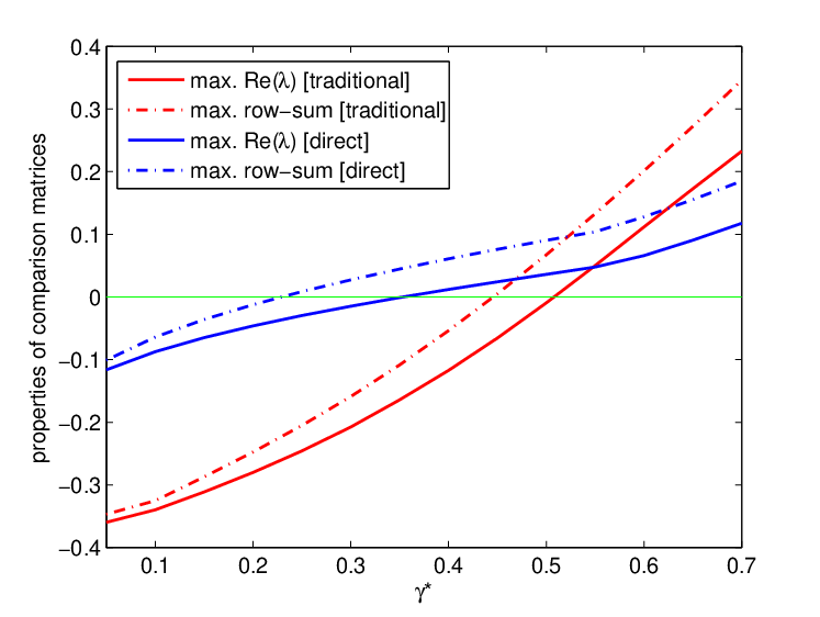
We note that both the maximum row-sum and the maximum $\text{Re}(\lambda)$ generally increases as $\gamma^{*}$ increases from 0 to 1, indicating that as the domain $\mathcal{D}$ ‘expands’, it becomes more difficult to certify stability. We also note that, for both approaches, the maximum row-sum becomes positive before maximum $\text{Re}(\lambda)$, indicating that the ‘invariance’ criterion is lost before the ‘Hurwitz’ criterion. Significantly, we also note that both the Hurwitz and invariance criteria are satisfied for a wider range of $\gamma^{*}$ in case of the direct approach than in the case of the traditional one. Thus, with regards to both the criteria, the direct approach is seen to perform better than the traditional approach.

Let us illustrate how this method can be used to certify exponential convergence of a given initial condition to the origin. The system dynamics is evolved against a randomly generated initial condition, and is found to be converging to the origin. Fig. 4 shows the evolution of the states belonging to subsystems - 2, 6, 7 and 8.

The initial condition yields the following level sets,

which is then used to define the domain $\mathcal{D}$, in (24). Then the SOS-based direct approach is used to compute the comparison matrix, $A\in\mathbb{R}^{9\times 9}$, with maximum $\text{Re}(\lambda)$ as -0.078, and $A\gamma^{0}<0$. The solution, $w(t)\in\mathbb{R}^{9}$, of the corresponding comparison equation $\dot{w}=A\,w\,,\,w(0)=\gamma^{0}$, is plotted against the actual Lyapunov level sets in Fig. 5, for subsystems 2, 6, 7 and 8.

The trajectories $w(t)$ exponentially converge to zero and, from Lemma 1, provide an upper bound on the corresponding subsystem Lyapunov function level sets.

When the same procedure is done with the traditional approach, we obtain a Hurwitz comparison matrix, $\tilde{A}$, with maximum $\text{Re}(\lambda)$ as -0.001, but with $\tilde{A}\left(\gamma^{0}\right)^{1/2}>0$, thus violating the invariance condition.

We have presented an SOS based direct approach to compute the linear comparison principle for stability analysis of interconnected systems. We have also discussed the traditional approach to obtaining the comparison equations, and shown how the direct approach can yield ‘better’, or less conservative, certificates of exponential stability. Using a network of Van der Pol systems we have presented a comparison of the two approaches. The proposed approach can be implemented on a suitable parallel platform where each row of the comparison matrix, corresponding to each subsystem, is computed in parallel.

A decentralized control framework can be visualized where each subsystem computes a local control law that will guarantee satisfaction of the Hurwitz and invariance conditions. SOS methods can be used to extend the stability analysis to higher order, and more general, comparison equations. Also, it would be interesting to see how the use of higher order (for example, quartic) Lyapunov functions in the comparison equation affects the conservativeness of the stability certificates.

References

- [1] A. M. Lyapunov, The General Problem of the Stability of Motion. Khatkov, Russia: Kharkov Math. Soc., 1892.
- [2] W. M. Haddad and V. Chellaboina, Nonlinear Dynamical Systems and Control. Princeton, New Jersey: Princeton University Press, 2008.
- [3] A. Papachristodoulou, J. Anderson, G. Valmorbida, S. Prajna, P. Seiler, and P. A. Parrilo, “SOSTOOLS: Sum of squares optimization toolbox for MATLAB,” 2013, available from http://www.eng.ox.ac.uk/control/sostools.
- [4] S. Prajna, A. Papachristodoulou, P. Seiler, and P. A. Parrilo, Positive Polynomials in Control. Berlin, Heidelberg: Springer-Verlag, 2005, ch. SOSTOOLS and Its Control Applications, pp. 273–292.
- [5] J. F. Sturm, “Using SeDuMi 1.02, a MATLAB toolbox for optimization over symmetric cones,” Optimization Methods and Software, vol. 11-12, pp. 625–653, Dec. 1999, software available at http://fewcal.kub.nl/sturm/software/sedumi.html.
- [6] Z. W. Jarvis-Wloszek, “Lyapunov based analysis and controller synthesis for polynomial systems using sum-of-squares optimization,” Ph.D. dissertation, University of California, Berkeley, CA, 2003.
- [7] M. Anghel, F. Milano, and A. Papachristodoulou, “Algorithmic construction of Lyapunov functions for power system stability analysis,” Circuits and Systems I: Regular Papers, IEEE Transactions on, vol. 60, no. 9, pp. 2533–2546, Sept 2013.
- [8] J. Anderson and A. Papachristodoulou, “A decomposition technique for nonlinear dynamical system analysis,” IEEE Transactions on Automatic Control, vol. 57, pp. 1516–1521, June 2012.
- [9] ——, “A network decomposition approach for efficient sum of squares programming based analysis,” in American Control Conference (ACC), 2010, June 2010, pp. 4492–4497.
- [10] D. Siljak, “Stability of large-scale systems under structural perturbations,” Systems, Man and Cybernetics, IEEE Transactions on, vol. SMC-2, no. 5, pp. 657–663, Nov 1972.
- [11] S. Weissenberger, “Stability regions of large-scale systems,” Automatica, vol. 9, no. 6, pp. 653–663, 1973.
- [12] A. N. Michel, “On the status of stability of interconnected systems,” Automatic Control, IEEE Transactions on, vol. 28, no. 6, pp. 639–653, 1983.
- [13] M. Araki, “Stability of large-scale nonlinear systems � quadratic-order theory of composite-system method using M-matrices,” IEEE Transactions on Automatic Control, vol. 23, no. 2, pp. 129 – 142, 1978.
- [14] R. Conti, “Sulla prolungabilità delle soluzioni di un sistema di equazioni differenziali ordinarie.” Bollettino dell’Unione Matematica Italiana, vol. 11, no. 4, pp. 510–514, 1956.
- [15] F. Brauer, “Global behavior of solutions of ordinary differential equations,” Journal of Mathematical Analysis and Applications, vol. 2, no. 1, pp. 145–158, 1961.
- [16] E. F. Beckenbach and R. Bellman, “Inequalities,” Spring-Verlag, New York/Berlin, 1961.
- [17] R. Bellman, “Vector Lyapunov functions,” Journal of the Society for Industrial & Applied Mathematics, Series A: Control, vol. 1, no. 1, pp. 32–34, 1962.
- [18] F. N. Bailey, “The application of Lyapunov’s second method to interconnected systems,” J. SIAM Control, vol. 3, pp. 443 – 462, 1966.
- [19] L. Jocic, M. Ribbens-Pavella, and D. Siljak, “Multimachine power systems: Stability, decomposition, and aggregation,” Automatic Control, IEEE Transactions on, vol. 23, no. 2, pp. 325–332, Apr 1978.
- [20] B. Van der Pol, “On relaxation-oscillations,” The London, Edinburgh, and Dublin Philosophical Magazine and Journal of Science, vol. 2, no. 11, pp. 978–992, 1926.
- [21] J.-J. E. Slotine, W. Li et al., Applied nonlinear control. Prentice-Hall Englewood Cliffs, NJ, 1991, vol. 199, no. 1.
- [22] P. A. Parrilo, “Structured semidefinite programs and semialgebraic geometry methods in robustness and optimization,” Ph.D. dissertation, Caltech, Pasadena, CA, 2000.
- [23] W. Tan, “Nonlinear control analysis and synthesis using sum-of-squares programming,” Ph.D. dissertation, University of California, Berkeley, CA, 2006.
- [24] A. Papachristodoulou and S. Prajna, “On the construction of Lyapunov functions using the sum of squares decomposition,” in Proceedings of the IEEE Conference on Decision and Control, Dec. 2002, pp. 3482–3487.
- [25] Z. J. Wloszek, R. Feeley, W. Tan, K. Sun, and A. Packard, Positive Polynomials in Control. Berlin, Heidelberg: Springer-Verlag, 2005.
- [26] A. Papachristodoulou and S. Prajna, Positive Polynomials in Control. Berlin Heidelberg: Springer-Verlag, 2005.
- [27] ——, “A tutorial on sum of squares techniques for systems analysis,” in Proceedings of the 2005 American Control Conference, June 2005, pp. 2686–2700.
- [28] M. Putinar, “Positive polynomials on compact semi-algebraic sets,” Indiana University Mathematics Journal, vol. 42, no. 3, pp. 969–984, 1993.
- [29] J.-B. Lasserre, Moments, positive polynomials and their applications. World Scientific, 2009, vol. 1.
- [30] M. Anghel, J. Anderson, and A. Papachristodoulou, “Stability analysis of power systems using network decomposition and local gain analysis,” in Bulk Power System Dynamics and Control-IX Optimization, Security and Control of the Emerging Power Grid (IREP), 2013 IREP Symposium. IEEE, 2013, pp. 1–7.
- [31] H. E. Bell, “Gershgorin’s theorem and the zeros of polynomials,” American Mathematical Monthly, pp. 292–295, 1965.
-C Proof of Lemma 2
Since and , we have