Why the laser linewidth is so narrow: A modern perspective
Abstract
We review and interpret a modern approach to laser theory, steady-state ab initio laser theory (SALT), which treats lasing and amplification in a unified manner as a non-unitary scattering problem described by a non-linear scattering matrix. Within the semiclassical version of the theory the laser line has zero width as the lasing mode corresponds to the existence of an eigenvector of the S-matrix with diverging eigenvalue due to the occurrence of a pole of the scattering matrix on the real axis. In this approach the system is infinite from the outset and no distinction is made between cavity modes and modes of the universe; lasing modes exist both in the cavity and in the external region as solutions satisfying Sommerfeld radiation boundary conditions. We discuss how such solutions can be obtained by a limiting procedure in a finite box with damping according to the limiting absorption principle. When the electromagnetic and matter fields are treated as operators, quantum fluctuations enter the relevant correlation functions and a finite linewidth is obtained, via a generalization of SALT to include noise (N-SALT). N-SALT leads to an analytic formula for the linewidth that is more general than all previous corrected versions of the Schawlow-Townes formula, and can be evaluated simply from knowledge of the semiclassical SALT modes. We derive a simpler version of this formula which emphasizes that the noise is dominated by the fluctuations in the polarization of the gain medium and is controlled by the rate of spontaneous emission.
I Introduction
The laser has been a critical enabler of the modern discipline of quantum optics via its highly monochromatic and intense emission properties. The physical understanding of steady-state laser emission has presented challenges since the early days after its invention, as first semiclassical [1, 2] and then fully quantum laser theories were developed [3, 4, 5, 6]. Although these theories were able to capture most of the relevant physics, they tended to incorporate some phenomenological or approximate steps due to the complexity of dealing with the full non-linear and space-dependent semiclassical or quantum laser equations. Over forty years ago, several pioneers of early laser theory, Lang, Scully and Lamb, addressed some of the weak points in the theory in a classic paper entitled,“Why is the Laser Line so Narrow? A Theory of Single Quasi-mode Laser Operation” [7]. This work was aimed at a fundamental challenge in laser theory, dealing with the openness of the laser system, which invalidated standard Hermitian modal decompositions appropriate for closed systems. Prior to this work essentially all theories were framed in terms of “quasi-modes” of the type studied by Fox and Li and were based on phenomenological modal equations with cavity damping inserted to represent the outcoupling of the modes [8]. The goal of Lang et al. was to go beyond these quasi-mode equations for the laser field amplitudes to a more fundamental description which included both the cavity and exterior regions explicitly (i.e. a model of “the universe”), and then work back from the modes of the universe to the quasi-modes of the cavity region alone. Using this approach the authors (1) “hope[d] to understand the mechanism leading to the extreme monochromaticity of the laser radiation”, and (2) “to investigate the sense in which the present calculation, which does not include the cavity dissipation as a phenomological loss mechanism, still leads to and implies a fluctuation-dissipation theorem” [7].
While this approach to understanding the laser equations was groundbreaking at the time, there has been much progress in laser theory in the subsequent years and it seemed to us a good time to re-examine these questions from a modern perspective. One reason for this is that during the past decade a new theoretical framework has been developed, known as the steady-state ab initio laser theory (SALT), which treats the openness of an arbitrary cavity exactly within the semiclassical theory [9, 10, 11, 12], and thus has provided new insights into lasing phenomena. The resulting non-linear SALT equations for steady-state lasing can be solved efficiently using a non-Hermitian basis set method and have been shown to agree to very high accuracy with brute force simulations of the atomic lasing equations [13, 14], including even N-level models with multiple independent lasing transitions [15]. The theory can also be generalized to treat injected signals (I-SALT), as will be relevant below [16]. Moreover, recently Pick et al. have added Langevin noise to the SALT equations (N-SALT) and, using the SALT steady-state lasing modes as a starting point, calculated the quantum-limited laser linewidth analytically [17]. Their analytic results have very recently been confirmed, again by direct simulations of the lasing equations, but with appropriate noise terms included [18]. It should be said that many aspects of the results obtained through SALT and N-SALT were anticipated by prior theoretical approaches, a partial list of which includes the work by Spencer and Lamb [19], Fu and Haken [20, 21, 22], and Henry [23]; however SALT and N-SALT appear to be the most general, flexible and inclusive formalism yet developed for steady-state lasing. It treats the fields over the entire “universe” from the outset, but in a different manner from Lang et al., and does not arrive at modal equations with damping in the conventional sense. We will now examine the questions raised by Lang et al. from the perspective of SALT and N-SALT.
II Lasers as Scattering Systems
II.1 Motivation and definition of the problem
Most early lasers emitted from lasing modes which were concentrated along some optical axis, e.g. the axis joining the centers of two mirrors or the geometric or index profile defining a waveguide or fiber, and so there was a tendency to develop laser theories focused on one-dimensional or axially symmetric equations, and this is overwhelmingly the type of formulation one finds in text books [24, 25, 26]. However in the past two decades a great variety of laser systems have been developed with complex two or three-dimensional cavities, such as microdisks and microspheres [27, 28, 29], micro-toroids [30], deformed (chaotic) disk cavities [31, 32, 33], photonic crystal defect-based and surface emitting lasers [34, 35, 36] and random lasers [37, 38, 39, 40, 41, 42, 43]. To describe such devices it was necessary to formulate laser theory in a manner that could both describe, and be implemented computationally, for cavities with an arbitrary geometry, and to include the full Maxwell wave equation, not its axial approximation.
Moreover, some of the new lasers (e.g. random lasers) are extremely open systems, not even cavities in the usual sense; nor do they always emit well-behaved narrow beams of light but rather generate complex emission patterns in two and three dimensions. Thus it was crucial to find a description which did not over-simplify the spatial properties of the cavities and emission patterns, and which hence treated the cavity boundary and outcoupling exactly. The solution to this challenge provided by SALT is to describe the laser as a scattering system. Any laser consists of two essential elements: a cavity region, given as a linear dielectric function, , which describes the scattering and confinement of photons, either injected externally or internally generated, and a gain region, containing the medium which will be pumped to provide optical gain (sometimes cavity and gain medium essentially coincide). To include all cases the “cavity” will refer simply to a singly connected region large enough to enclose all the regions in which ; and for simplicity we will assume the gain medium is fully contained within this region as depicted in Fig. 1.

The laser so defined can function both as an amplifier of input radiation (when the gain medium is inverted) and as a self-organized oscillator/source of radiation in the absence of input, above the first threshold for lasing. From this point of view the laser is a scattering system which both scatters and amplifies input radiation, and also, at discrete frequencies, scatters specific internally generated modes of outgoing radiation when sufficiently pumped. However unlike linear scattering systems, the laser is subject to non-linear saturation effects which are fundamental to its stability and must be taken into account.
Other non-linear effects within lasers, such as four-wave mixing, can destabilize their simple harmonic time-response, but these effects are neglected in SALT, and also (typically) in the earlier laser theories which motivated the work by Lang et al. [7]. Leaving out such effects is equivalent to assuming a stationary inversion density, giving rise to a gain susceptibility which does not mix frequencies. This assumption is always valid for single-mode lasing and amplification, which will be the focus of this work; it is also valid under certain rather general conditions for multimode lasing in microlasers, and SALT has been shown to apply quantitatively to such cases [13, 14, 15, 16].
Before proceeding, it should be mentioned that the input/output theory developed by Collett and Gardiner (and others) also considers the cavity to be a scattering element [44, 45] and is able to treat the full quantum operator properties of the scattered fields. This approach has certainly contributed to our understanding of open quantum systems and the role played by the reservoirs and noise processes. However, while there has been substantial effort expended to describe lasing within this framework [46, 47, 48, 49], it remains an open problem how to include the strong non-linearities present in active lasing systems in this formalism; whereas at the semiclassical level this is done quite accurately by SALT.
II.2 Scattering in the SALT formulation
Initially we focus on the single-mode lasing case, as was done by Lang et al., so that the positive frequency component of the electric field will be given by:
| (1) |
where the real number, , is either the input radiation frequency (for the amplifier) or the unknown frequency of the laser oscillator, which must be self-consistently determined. is the unknown spatial lasing (or amplified) mode, not assumed to be equal to any passive cavity mode or quasi-mode and is also self-consistently determined; such lasing/amplifier modes describe the solution over all space, not just inside the cavity.
Assuming stationary inversion and neglecting quantum and thermal fluctuations, we can describe for an arbitrary laser by a non-linear wave equation of the form:
| (2) |
where , and is the complex, frequency-dependent saturable gain susceptibility, which can be calculated for an arbitrary N-level atomic gain medium in steady-state [14]. For the case of a two-level gain medium it takes the form
| (3) |
where is the pump parameter (proportional to the inversion), is the dephasing rate of the polarization, is the atomic resonance frequency, and is a Lorentzian centered at . and are measured here in appropriate dimensionless units [13], and this form assumes that there is only one mode, either lasing or amplified, active in the medium. (This is the only case we will consider explicitly here, but we will review the more general multimode SALT formalism in Appendix A). The non-linear gain susceptibility represents the polarization of the gain medium and is the source of the amplification and (above threshold) of laser emission. The lack of any Langevin force terms in Eq. (2) is a result of the semiclassical approximation, in which the operators for the electromagnetic and polarization fields are replaced by their average values, eliminating the effects of quantum and thermal fluctuations. Such terms are taken into account in N-SALT, which will be discussed briefly in Sec. VII, but were neglected (intentionally) in the work of Lang et al.
Assuming the system is pumped below the first lasing threshold and the inputs are small enough to generate negligible saturation of the gain, this equation defines a linear non-unitary scattering (S-)matrix for input fields. Depending upon the geometry there are different natural basis states describing input and output modes, , , from and to infinity, i.e. sufficiently far away from the cavity region,
| (4) | ||||
| (5) |
If the pump is strong enough to invert the medium and create gain at the input frequency, the S-matrix will be amplifying, with eigenvalues greater than unity. When functioning as an amplifier the boundary conditions are familiar: an input wave from infinity interacts with the cavity plus gain medium, scattering according to the appropriate dielectric or metallic boundary conditions in different regions of the cavity and giving rise to an outgoing wave which differs from passive scattering in that it is amplified and more photon flux emerges from the scattering region than enters it. The case of large inputs leading to a saturated gain and the resulting non-linear S-matrix can be handled by I-SALT and will be included in the discussion below.
As noted, In this formulation there is no distinction between cavity modes and modes of the universe, every amplified mode exists inside and outside the cavity as a steady-state scattering solution. However we now consider to the more challenging and subtle case of laser oscillation in the scattering picture.
III Quasi-modes, Resonances and Quasi-bound States
Any scattering region of finite extent with a real potential or dielectric function, and hence with a unitary S-matrix, will have associated with it resonant solutions; i.e. stationary solutions at discrete complex frequencies which are purely outgoing. It is easiest to think of these as evolving out of the bound states of the system at real frequencies, , which would occur if the region were surrounded by a perfect lossless reflecting barrier. As the reflectivity of the fictitious barrier is reduced from unity to zero these real frequency solutions, corresponding to standing waves, evolve into complex frequency solutions with a substantial outgoing wave component (and no incoming wave from infinity). Due to the purely outgoing boundary conditions it can be shown that the imaginary part of the frequency must be negative, and the S-matrix, continued to complex frequencies, will become infinite with simple poles at . Hence these purely outgoing solutions are discrete and countably infinite, in one to one correspondence with the bound states of the closed cavity.
In the asymptotic region the frequency and wavevector of the solutions are linked by the dispersion relation and the sign of will cause the corresponding spatial solution to grow exponentially at infinity and carry a diverging outgoing photon flux. Hence these solutions are not physically realizable, but have physical significance because the S-matrix will have a resonant response near the real values , with a bandwidth given by (assuming well-separated high finesse resonances). The corresponding spatial solutions are referred to by various terms: quasi-modes, quasi-bound states and resonances. Historically the use of multiple terms seems to have arisen from the transition from 3D confinement, as e.g. in a microwave resonator, where the connection to bound states is more apparent, to open, axial mirror-based resonators, where the resonances perpendicular to the mirror axis are essentially absent, and the Fox-Li method was developed to determine the high resonances. However there is no fundamental difference between the various types of outgoing solutions: they all correspond to poles of the passive cavity S-matrix.
Such states also are very well-known from quantum scattering theory (where they are usually referred to as quasi-bound states), and are often considered to be physical states because if an initial condition is given corresponding to the quasi-bound state truncated to the “cavity region”, it will leak out to infinity with a rate given by (this property was explicitly demonstrated for the one-dimensional cavity treated by Lang et al.). However in this context we would like to emphasize that the true quasi-bound states, including the exponentially growing component at infinity, are not physically realizable steady-state solutions and cannot correspond to the lasing mode. Also, since they occur at the poles of the S-matrix for the passive cavity, they can only describe the properties of the passive cavity, independent of the gain medium and spectrum. Thus using “quasi-mode” also as a term for the lasing mode in the presence of gain can, and in our view often has, led to confusion.
IV Threshold Lasing Modes and Constant Flux States
However, as described above, the properties of the laser/amplifier are not governed by a unitary S-matrix once the complex gain susceptibility is taken into account. This complex susceptibility violates the Hermiticity of the wave equation even for the closed cavity and invalidates the standard modal decomposition. But it makes possible purely outgoing solutions at real frequencies, which hence are physical solutions over all of space. The non-equilibrium steady-state gain susceptibility depends on the pump level, with its imaginary part changing sign from positive (absorbing) to negative (amplifying) at the transparency point, at which the upper and lower lasing levels are equally occupied and the susceptibility vanishes. At this pump value the poles of the cavity with gain coincide again with those of the passive cavity. As the pump is increased beyond the transparency point, all of the passive cavity poles continue to exist, but typically they move up in the complex plane towards the real axis [12, 50, 51], at a rate that depends on their position in the gain spectrum. The S-matrix of the amplifier can be measured for real frequencies as the pump increases, and the height of the resonances corresponding to each pole increases (the transmitted flux is greater than the incident flux due to amplification), while their width decreases (gain narrowing), because the effective loss rate is proportional to the imaginary part of the pole frequency, which is decreasing. If there is no input to the amplifier then there is still no emitted field and no indication within semiclassical theory of the approach to lasing (although when quantum fluctuations are included there will be enhanced noise, amplified spontaneous emission (ASE), near the gain center). If lasing is achieved, one of the poles of the S-matrix reaches the real axis, gain completely balances loss, and we have a zero width resonance on the real axis. This process is demonstrated in Fig. 2 for a non-trivial two-dimensional cavity, a chaotic “D-shaped” dielectric cavity [33], where each pole is seen to move towards the real axis an amount proportional its distance from the center of the gain curve and one of the poles experiences enough gain to reach threshold.

It first may seem that we are back at the familiar situation of true bound states, which correspond to poles on the real axis, but this is not so. In the former case there is no photon gain and one simply has a decaying standing wave pattern, trapped in some region of space. Here we have a different type of object, which we call a “threshold lasing mode” (TLM). This type of solution never occurs in Hermitian theories, a purely outgoing solution at real frequency; it reflects the fundamentally non-Hermitian nature of the electromagnetic wave equations with a complex susceptibility, which is an effective theory in which the matter degrees of freedom are hidden. Such a solution is characterized by a steady-state photon flux out to infinity, but with no unphysical growth of intensity outside the cavity and an emission pattern corresponding to the eigenvector of the S-matrix with a diverging eigenvalue. It is an example of a constant flux (CF) state: photons are generated within the cavity but are conserved outside the cavity, hence corresponding to a true physical lasing solution [9, 11, 12]. In Appendix A we will show that each TLM is just one member of a complete biorthogonal basis set of CF states which forms a natural basis set for describing the non-linear lasing solution above threshold.
However we still have a conceptual problem: the linear S-matrix for this amplifier is now infinite at the lasing frequency. Within linear theory any input would be infinitely amplified, violating conservation of energy. The resolution of this dilemma is that infinitesimally above threshold the saturating non-linearity kicks in and stabilizes the solution. In fact the steady-state lasing amplitude rises smoothly from zero and has no jump at threshold, just a discontinuous derivative. Even though formally the S-matrix has a pole fixed on the real axis above threshold, any input wave at the lasing frequency simply increases the gain saturation and doesn’t lead to a runaway of the output. Strictly speaking, any such input actually forces the pole off the real axis, as we will show with an example in Sec. V. Hence the non-linearity is essential for stablizing the linear CF solution. However, the actual solution near threshold is accurately described by the single TLM calculated from the linear wave equation with gain, since the saturation term is not strong enough to change the spatial form of the solution significantly.
Returning to the fundamental question of modes of the universe vs. quasi-modes of the cavity, we summarize the SALT perspective.
- •
If one treats lasers as unbounded scattering systems from the outset, all solutions are defined both inside and outside the cavity region and there is no distinction between cavity modes and modes of the universe.
- •
If the laser is functioning as an amplifier, the solutions are simply amplified scattering states determined by the boundary conditions in the cavity region and the degree of gain at the input frequency.
- •
If the laser is functioning as a self-organized oscillator the solutions are purely outgoing states corresponding to an eigenvector of the linear scattering matrix with diverging eigenvalue due to the existence of a pole on the real axis. Such solutions require the presence of the saturating non-linearity to be physically stable.
- •
For any given cavity and gain susceptibility such purely outgoing states can only occur at discrete frequencies because they arise from moving the discrete poles of the passive cavity onto the real axis. Within semiclassical theory (neglecting quantum and thermal fluctuations of the fields) these solutions have precisely zero linewidth.
We reserve the term “lasing mode” for these special discrete solutions.
In summary then, our response to the question “why is the laser linewidth so narrow?” is that indeed this is due to the extreme limit of gain narrowing: only at discrete frequencies can the linear gain diverge and generate self-organized oscillation. As we will show in the next section, this zero-width resonance cannot be observed with an input signal, i.e. in amplification mode. However these perfectly monochromatic purely outgoing solutions can be found by SALT and have been verified by brute force FDTD simulations of the laser equations for many examples [12, 14, 15]. Such infinitely sharp lines are not of course obervable in true laser emission due to quantum fluctuations as we will discuss in Sec. VII. However the smallness of these quantum effects lead to the extraordinary narrowness of the resulting lines, often many orders of magnitude narrower than the passive cavity resonance linewidths.
The effects of quantum fluctuations were intentionally not included in the work of Lang et al., who thus also found a delta function laser line within semiclassical theory. In their approach they find that this extreme narrowing of the passive cavity resonance can be regarded as a “mode-locking effect” in which all of the modes of the universe within the passive cavity resonance linewidth contribute to one lasing quasi-mode with a single frequency. This point of view emerges from a limiting procedure in which a finite system with quantized electromagnetic modes is studied and at the end the system size is taken to infinity in the presence of small fictitious absorption to damp out reflections from the boundaries as they tend to infinity. The conditions for this procedure to reproduce the correct infinite system behavior are discussed in Sec. VI below. We note that Lang et al. expressed dissatisfaction with invoking gain narrowing to explain the laser linewidth, because in their view such arguments (at the time) did not take into account the non-linearity of the problem. However the conceptual framework of SALT/I-SALT, outlined here, does take non-linearity into account, essentially exactly, for single-mode lasing. We will now illustrate the previous concepts with a concrete one-dimensional example, very similar to the one studied by Lang et al., in the process making all of our statements above mathematically precise.
V Lasing modes as zero-width resonances: A simple example
The example studied by Lang et al. was a one-dimensional cavity of length , with perfectly reflecting mirrors at and a partially reflecting delta function mirror at , as shown in Fig. 3. The “cavity” is the region and the “universe” is the region, , where in treating lasing a small uniform absorption is added over all space, the limit is taken, and lasing emission is in a single direction towards . For such a system the passive cavity will have a reflection coefficient of modulus unity at all frequencies, and resonant reflection will be distinguished only by a long delay time in reflection and an associated build-up of field intensity in the cavity. We prefer to make a small modification of the Lang et al. example and study a symmetric two sided partially transmitting (Fabry-Perot) cavity with laser emission to , and with passive cavity resonances distinguished by enhanced transmission, reaching unity at the center, and with width, . As with the Lang et al. example, the electromagnetic part of the problem will be described by the scalar Helmoltz equation with gain. However, unlike Lang et al., no limiting procedure is applied; our system is infinite from the start and no fictitious absorption is added to avoid reflections from perfect mirrors far away from the cavity. Hence, consistent with our scattering approach, we start from continuous solutions for the passive cavity “universe”, and will impose outgoing boundary conditions at infinity on the lasing solutions.

We begin by reviewing the properties of such a one-dimensional optical cavity. In Fig. 4 we plot the transmitted intensity of an incident signal through the passive cavity at frequency . As expected we observe a series of resonances of the cavity, spaced by the free spectral range, , with a width given by the passive cavity decay rate , where is the length of the cavity. The incident and reflected waves on the left side of the cavity satisfy a continuity boundary condition, with both incoming and outgoing components, whereas the transmitted wave leaving the right side of the cavity also is continuous but in addition is purely outgoing.
Any purely outgoing monochromatic wave is described mathematically by the Sommerfeld radiation condition [52],
| (6) |
in which , , and is the dimensionality of the system. In one dimension the external waves are simple plane waves (and not e.g. cylindrical or spherical waves) and the Sommerfeld condition can be imposed anywhere outside the boundary; thus at the boundary on the right side of the cavity the field must be an outgoing plane wave, satisfying,
| (7) |

As noted, lasing would correspond to a solution satisfying a purely outgoing boundary condition on both sides of the cavity (or in all directions in higher dimension). If we attempt to impose this boundary condition on the passive cavity we find that no solutions are possible at real frequencies, but there are discrete periodically spaced solutions at
| (8) |
as shown in Fig. 4. The discreteness of the frequencies is a direct consequence of the Sommerfeld condition which can only be satisfied when there is constructive interference in the cavity. The fact that all the resonance frequencies have the same imaginary part is not generic, but is particular to one-dimensional cavities of this type. As noted above, the presence of these purely outgoing (pole) solutions leads to resonant transmission on the real axis centered at with width . Applying the Sommerfeld condition to the outgoing solutions , and the relation implies that at , the unphysical divergence we alluded to above.
In order to find normalizable physical solutions which are purely outgoing (i.e. lasing solutions) we need to add the effect of the gain medium to the cavity dielectric function in the form of as defined in Eq. (3) above. For this simple one dimensional scalar model (similar to Lang et al.), below threshold, the electric field satisfies
| (9) |
with the Sommerfeld boundary condition, where now the index of refraction , and the gain non-linearity is neglected, because we are below threshold and these are not yet physically allowed solutions (they are simply modified active cavity resonances). Note that the solutions inside the cavity here take the form , i.e. they are trigonometric functions of a complex argument. This will remain true at threshold and is a key point which holds more generally: the electric fields for the physical system with gain cannot be purely real; if they were real they would conserve photon flux and describe true standing waves, whereas lasing or amplified modes must have running wave components. Any model which finds real spatial solutions for lasing or amplified modes has made an approximation. Such approximations have often been made in laser theory, including by Lang et al. [7, 53, 54, 55] (see further discussion in Sec. VI).
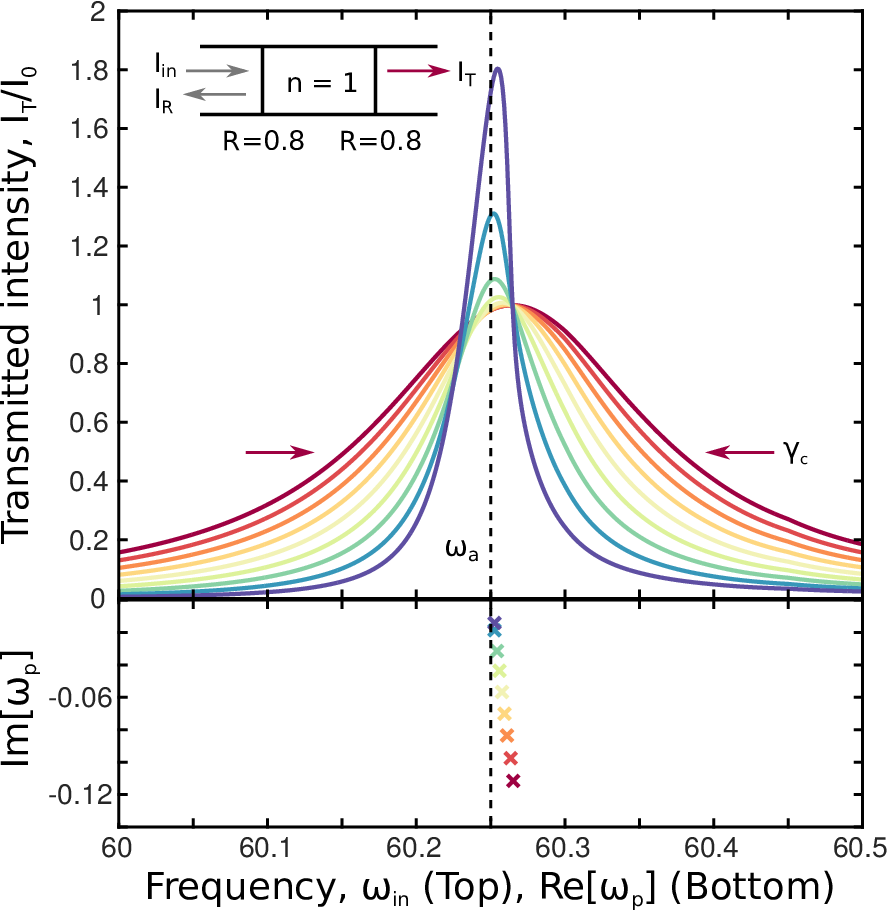
When we add the gain medium to the cavity and pump above the transparency point the imaginary part of corresponds to amplification. This has an immediate effect, causing the poles to move upwards, as discussed earlier and as shown for this specific cavity in Fig. 5. While the pole solutions are still not physically realizable, we can observe a change in the cavity properties via the behavior of the transmission resonances at real frequencies. To calculate this effect accurately with a finite input wave we must now use the full saturable gain susceptibility of Eq. (3). The simulations shown here are performed using I-SALT which provides a nearly exact description of the steady-state single-frequency response of an active optical cavity to injected signals and any self-generated lasing signals [16], including the spatial degrees of freedom. SALT and I-SALT are reviewed in more detail in Appendix A.
As the pole rises towards the real axis the amplified resonance narrows. Due to the frequency-dependent saturation of the gain medium, as already noted, injected signals with different frequencies will induce somewhat different trajectories for the pole in order to maximize the effective gain [16]. These are essentially line-pulling or pushing effects of the gain medium, which for a single frequency are always towards the atomic transition frequency. In the active cavity with dispersion, the precise width of the transmission resonance can no longer be defined as the distance of the pole from the real axis, as probing different frequencies will yield slightly different distances of the pole from the real axis. These line-pulling effects lead to the mild asymmetry in the series of curves shown in Fig. 5.
The bluest (and narrowest) curve shown in Fig. 5 corresponds to a pump value just above the non-interacting first lasing threshold. This may seem initially puzzling; wasn’t the lasing threshold the point at which the pole reaches the real axis? That definition only applies when there is no input signal. With an input signal, even at the lasing frequency, the saturation of the gain medium prevents the pole from reaching the real axis, keeping the response finite, and the amplifed resonance retains a non-zero width.
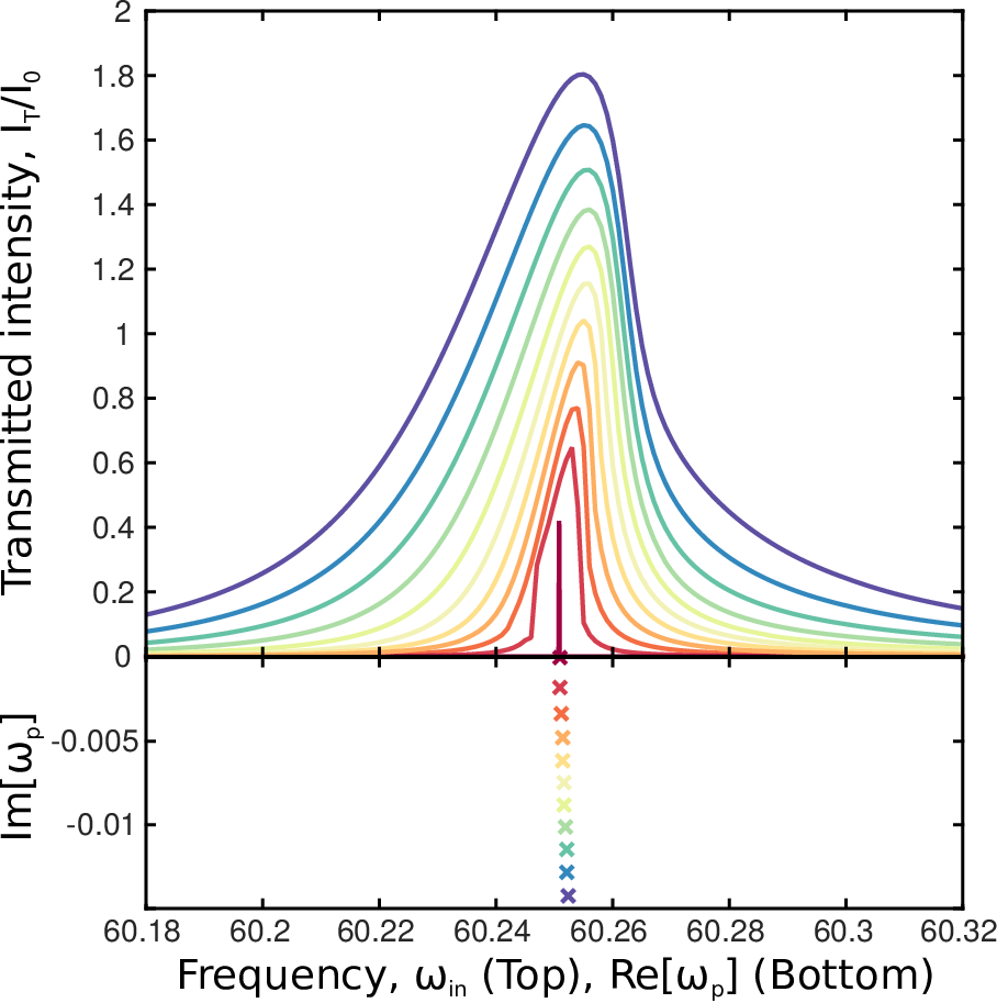
To see the true zero-width semiclassical lasing solution we slowly turn off the incident signal with the pump held above the first lasing threshold. With this protocol we see that the transmission resonance width continues to narrow, as shown in Fig. 6, while the pole continues to move towards the real axis. As the injected signal is turned off, the pole reaches the real axis and the cavity begins to undergo self-organized lasing action, shown as the reddest curve in the top panel of Fig. 6. This curve has precisely zero linewidth; no radiation comes out of the cavity except at this single frequency without input waves (assuming effectively zero temperature in the cavity and neglecting quantum fluctuations until Sec. VII). This effect can never be fully achieved through gain-narrowing of an amplified input signal, for the reasons we described above: gain saturation forces all poles off the real axis. Hence this effect does require correct treatment of the non-linearity as stated by Lang et al. However we have shown here that it is possible to treat the non-linearity exactly at each stage and explain the zero width of the laser line quantitatively.
The model we have treated here is essentially the same as that treated by Lang et al. except for the pedagogical difference of choosing a two-sided cavity in which one can study transmission resonances; in the next section we will study exactly the model of Lang et al. by a different but equivalent method. As noted, in the standard SALT approach the system is infinite from the outset and there is no dissipation outside the cavity, which is in our view the most natural model for a real laser system. In contrast, Lang et al. place their cavity in a much larger box which eventually will be taken to infinite size, and add dissipation external to the cavity, intended to damp unphysical reflections from the boundaries of the larger fictional box. We will discuss the effects of this difference in the next section.
VI Lasing modes and the Limiting Absorption Principle.
While it is clear that lasing modes should satisfy the purely outgoing (Sommerfeld) boundary condition, this leads to a rather unfamiliar description of the spatial behavior of the lasing modes in terms of functions that are not power orthogonal, but instead satisfy a biorthogonality condition [25, 56, 57]. Basis functions of this type, the CF states [9, 10, 11, 12], are central to the standard computational algorithm of SALT. The approach taken by Lang et al. of beginning with a finite system and adding damping to remove the effect of the boundaries of the system is an alternative which has evolved into the well-developed computational technique of surrounding a cavity or region of emitters with a perfectly-matched (damping) layer (PML). When done correctly this can reproduce the imposition of Sommerfeld conditions to arbitrary accuracy. In fact, newer computational methods for solving the SALT equations [58] make use of PMLs and do not impose the Sommerfeld boundary conditions in the straightforward manner of matching to outgoing solutions at a last scattering surface as did the earlier methods of satisfying the SALT equations [11]. The PML approach gives essentially perfect agreement with the Sommerfeld approach to SALT.
However, as noted above, the correct lasing solutions must be complex functions in space, so as to represent the non-zero photon flux, which grows inside the cavity and remains constant outside. For the simple 1D cavities studied here and by Lang et al., this means that the spatial solutions inside a constant index cavity must be trigonometric functions of complex argument, corresponding to exponential growth towards the mirrors as well as oscillation. However in the work of Lang et al. they find a lasing mode of the form for , where is the difference between gain and loss, is the lasing frequency, is a constant, and is the real wavevector corresponding to the passive cavity resonance frequency, . Since the spatial part of this function is real, it does not capture the photon flux through the partially transmitting mirror and is only an approximation to the complex sine wave solution which is correct for this one-sided cavity.
In our view the origin of this problem is the neglect of the Limiting Absorption Principle [59, 60, 61], which gives the correct mathematical procedure for recovering the Sommerfeld radiation condition from a finite system. Lang et al. solved the spatial part of the problem for finite , finding the quantized Hermitian basis states for the whole passive system (“modes of the universe”) and then addressing the lasing problem within this Hermitian basis set. Effectively the spatial part of the problem is fixed at finite , and a small absorption, , is subsequently added everywhere in the universe so as to eliminate the effect of reflection from the fictitious perfect mirror at . For this procedure to work one needs to solve the spatial problem with the finite damping, and carefully take the limit prior to ; this requirement is known as the Limiting Absorption Principle (LAP). From a practical computational point of view the LAP means that one needs to solve the non-Hermitian spatial problem with Dirichlet (or other linear homogeous) boundary conditions and finite damping, while maintaining the condition . The solutions so obtained have only exponentially small sensitivity to the presence of the boundary and reproduce to high accuracy those obtained by actually imposing directly the Sommerfeld conditions. Hence they are significantly different from the Hermitian solutions calculated before the damping is added (or when the limits are taken in the opposite order), which can carry no net flux as they are bound states. The modern PML techniques are a means for introducing non-uniform absorption which is impedance matched so that reflections are negligible even when is not very large and one reproduces the Sommerfeld solutions with a much smaller and manageable computational cell. But the principle is basically the same: in order to get the correct spatial solutions one must treat the non-Hermitian problem with damping from the outset.
To illustrate this explicitly we briefly analyze the Lang et al. system from this point of view. The system is the one-sided cavity between attached to the “universe” between , as shown in Fig. 3, with perfect mirrors (Dirichlet boundary conditions), , where is the electric field of the system. Before adding the gain and considering lasing, we explicitly include the weakly absorbing material uniformly in the universe, and focus on the region external to the cavity. The wave equation in this region is written as,
| (10) |
We expand the field inside of the system in terms of a set of basis functions, , so that , and solve for the form of these basis functions in the universe region as,
| (11) |
where we have expanded the exponent for . The coefficients and and the quantized values of are set by the boundary conditions , , and the matching conditions at , and will vary with , and the transparency of the mirror at the origin.
We first apply the LAP to obtain the Sommerfeld solution for this problem, taking the limit prior to . Performing the limits in this order on the solution of , Eq. (11), one finds that to satisfy the Dirichlet boundary condition, , we must choose , as the term multiplying this coefficient is diverging as for finite . Then, with the spatial limit taken, we can safely reduce the absorption in the problem to zero, recovering
| (12) |
finding that all of the solutions of our problem are purely outgoing from the cavity, consistent with the Sommerfeld radiation condition, Eq. (6). However, if these two limits are taken in the opposite order, setting the absorption to zero before letting the length increase to infinity, we find that
| (13) |
which is exactly the result of Lang et al. (outside the cavity region). With this result the matching to the cavity allows for real sine wave solutions, whereas with the outgoing solutions only complex sine waves are allowed in the cavity. The complex sines provide the outgoing flux at the partially transmitting mirror which is needed for continuity with the field outside the cavity.
These conclusions can be further reinforced by directly solving for the eigenfunctions of the finite system studied by Lang et al., shown in the three panels of Fig. 7. As is increased, the modes of this finite system separate into two sets. One set consists of discrete isolated solutions with smaller imaginary frequency (damping); the number of such solutions does not change with increasing . The second set has larger damping, and gets denser and denser, forming a psuedo-continuum as is increased. The first set corresponds precisely to the complex resonance frequencies of the passive cavity, as can be confirmed by plotting the known resonances of the cavity given by Eq. (8), shown in Fig. 7(c). The spatial functions corresponding to the passive resonances are identical to the resonant solutions of the infinite system without damping inside the cavity, as there is no loss there, and the boundary condition at the mirror is the same. Outside the mirror these solutions experience a damping not present in the infinite system and hence decay slowly as they propagate outwards. On the scale shown in the top panel of Fig. 8 one sees only that the outgoing boundary condition is satisfield and not the weak decay. In contrast, the spatial solutions corresponding to the dense set of damped modes of the universe can be seen in the bottom panel of Fig. 8; they form standing waves outside the cavity, with small leakage into the cavity, and do not satisfy the purely outgoing conditions. Hence simply discarding the latter and keeping the first set is equivalent to finding the Sommerfeld solutions of the passive problem without damping, in the vicinity of the cavity.
Finally, we can make contact with the SALT approach by adding gain (taken to be uniform for convenience) in the cavity region while leaving the damping present outside the cavity. The added gain has a much bigger effect on the cavity resonance solutions which have high amplitude there, than on the external standing wave solutions. For large enough gain one of the cavity resonances can reach the real axis and will then correspond to a threshold lasing mode for uniform gain, as shown in Fig. 7c (green crosses). This is the essence of the method adopted in Ref. [58] except in that work a PML damping layer is used for higher computational efficiency and the saturating non-linearity is taken into account. Thus the Lang et al. method agrees with the SALT approach if care is taken to apply the limits in the right order.


VII Quantum limited laser linewidth: an alternative form
Since this paper is devoted to the “SALT perspective” on the laser linewidth, we include here a section on the finite laser linewidth due to quantum fluctuations, which has recently been addressed within two different generalizations of SALT, one based on input-output theory [50, 51] and another based on non-linear perturbation theory around the SALT solution [17]. The fundamental origin of a finite quantum linewidth for the laser is the presence of spontaneous emission, which leads to random jumps in the time-dependent phase of the output field. The resulting phase diffusion is linear in time and the phase diffusion coefficient determines the intrinsic linewidth. The basic physical understanding of this goes back to the seminal work of Schawlow-Townes [62], which was subsequently substantially extended by Lax, Henry, Petermann and many others.
Traditionally, the Schawlow-Townes (ST) linewidth is written in terms of the cavity decay rate, , as
| (14) |
where is the lasing frequency and is the total output power. Here we have chosen to include in the ST formula the “incomplete” inversion factor, , which is sometimes treated as a correction to it ( measures the degree of inversion of the laser frequency and tends to unity when the lasing transition is completely inverted, the limit assumed by Schawlow and Townes in their original work) [63].
As discussed extensively above, semiclassical laser theory neglects quantum effects such as spontaneous emission and leads to a delta function linewidth. In order to go beyond this one needs to treat all three fields, the electromagnetic field, the polarization, and the inversion as quantum operators and consider their higher moments. The laser linewidth will be obtained from the correlation function of the electric field near the lasing frequency. It is well known that the effects of these quantum fluctuations can be captured by adding appropriate Langevin (random) noise terms to the equations of motion for the three fields [64]. These noise terms will be related to the dissipation and amplification in the system by the appropriate fluctuation-dissipation relations. This was one of the questions raised in the original work by Lang et al. It is now understood that semiclassical theory violates these relations but they are restored by including the Langevin terms. The recent work by Pick et al. [17] provides the most complete treatment of these noise terms and the formalism they develop is referrred to as N-SALT (SALT + noise).
Pick et al. begin with the time-dependent wave equation for the field and add the appropriate noise term
| (15) |
in which is the total effective noise driving the field in the cavity in units of electric field. Since this random drive is broadband, it is no longer possible to assume a monochromatic steady-state exists as we do in semiclassical theory. However only the noise near the lasing frequency is strongly amplified and by expanding the field around the SALT steady-state solution one can derive non-linear coupled mode type equations which permit ab initio calculation of the relevant correlation functions and hence of the most general form of the laser linewidth yet derived [17]. This form includes all of the important corrections to the ST formula: the correction due to relaxation oscillations ( factor) [65, 23], due to openness of the cavity (Petermann) factor [66, 67, 68, 56, 57], due to dispersion (bad-cavity factor) [63, 69, 70, 71, 72], and corrections not previously studied due to the spatial variation of [63]. We will not describe this formalism in any more detail here, but will briefly reproduce the essential result at the end of this section.
However, in this section we would like to make a different conceptual point, not discussed in the earlier papers, relating to the interpretation of the Schawlow-Townes formula. It seems initially puzzling that the noise due to spontaneous emission in the gain medium should lead to the standard ST formula, which is expressed only in terms of the passive cavity linewidth, , the total output power, and the lasing frequency. One would expect the spontaneous emission rate to appear as a fundamental quantity, not the cavity decay rate; and here we will show that the ST linewidth can (and perhaps should) be written in an equivalent form where this is the case.
The total Langevin force, , in units of the quantized field amplitude operator, , has a direct contribution from the amplitude fluctuations of the field, , due to quantum fluctuations from outside the cavity, but has also has indirect contributions from Langevin forces driving the atomic polarization and inversion, and respectively [64],
| (16) |
where the summation runs over all of the atoms in the cavity at locations and
| (17) |
is the dipole coupling element for the quantized electric field. is the dipole matrix element for the lasing transition, and is the normalized mode profile, , of the electric field at frequency . The correlation function for the total effective Langevin force can then be calculated [64] as,
| (18) |
in which is the number of thermal photons at the lasing frequency, is the dephasing rate of the polarization, and is the inversion of the th atom, which would relax to the steady-state value of in the absence of an electric field at the rate . We have also simplified by assuming the lasing signal to be on resonance with the atomic transition, , and that the dipole matrix element and field are co-linear, .
The first term in Eq. (18) corresponds to the contribution from thermal and zero point fluctuations from outside the cavity to the field inside the cavity; as such it is controlled by the decay rate of the cavity, . The second and third terms stem from spontaneous emission events leading to the dephasing of the atomic polarization, and these terms depend on the parameters of the gain medium. For optical frequencies, the number of thermal photons present is negligible, so the direct field fluctuations do not have any effect on resulting linewidth. Moreover, for most lasers (class A and B) [73], , so that only the second term in Eq. (18) remains,
| (19) |
Assuming that the atoms are uniformly distributed over the cavity, the sum over the atoms in the cavity can be converted into an integral,
| (20) |
where () is the density of atoms in the upper (lower) lasing level, and . Equation (20) now expresses the Langevin force in terms of the incomplete inversion factor [63],
| (21) |
Traditionally at this step the atomic populations are approximated to be uniform in space which clamps the inversion to its value at the lasing threshold, [64]. In this approximation, the integral in Eq. (20) becomes just , and can be related back to the cavity decay rate by
| (22) |
which states that at the lasing threshold, gain must equal loss. Using this approximation contributes one factor of in the standard ST linewidth formula, Eq. (14). However this is a rather crude approximation. Due to spatial hole-burning the atomic populations generally vary substantially in space, and as a consequence the overall inversion is not clamped at the threshold value.
Using Eq. (22) obscures the fact that the physical origin of the noise is spontaneous emission in the gain medium. It then is more natural to relate the linewidth to the rate of spontaneous emission, , which can be calculated from the rate of stimulated emission, [15], as
| (23) |
where is the number of photons in the steady-state lasing field, and is related to the intensity by . Thus, we can rewrite Eq. (20) in terms of the rate of spontaneous emission, keeping the full space dependence of the problem, as
| (24) |
As noted above, the coefficient of the Langevin noise determines the laser linewidth by standard manipulations. Using the more correct form of this coefficient above leads to a quantum-limited linewidth,
| (25) |
Typically, the next step is to relate this to the total output power of the cavity via
| (26) |
which is also only an approximate relation, neglecting spatial variations of the intensity. Using both of the approximations mentioned above and some other simplifications valid for high cavities (and neglecting the amplitude contribution contained in the factor), one then arrives at the standard ST linewidth form, Eq. (14).
However, the actual power emitted can be calculated using the true spatially-varying fields using Poynting’s theorem [74], as
| (27) |
Using specific form of the imaginary part of the dielectric function for a two-level gain medium (and using real units, not SALT units), the linewidth can then be written as
| (28) |
Here we have derived a more physically intuitive and accurate form of the laser linewidth formula in which the critical role of spontaneous emission in the gain medium leaps out: the linewidth is determined by the spatially-varying, mode-dependent spontaneous emission rate and by the steady-state saturated inversion in the presence of spatial hole-burning. Only if one makes the approximation of does this reduce to the standard Schawlow-Townes formula, and in making this substitution one tends to hide the true origin of the linewidth, which is spontaneous emission.
While the above argument captures the basic physics of the ST formula in an improved form, it is not a rigorous general result, as is the formula derived by Pick et al. [17], which includes essentially all known corrections in a more accurate form. However the N-SALT linewidth does have the same general features as our simpler result, Eq. (28), and for a single lasing mode can be written as [17],
| (29) |
where is the normalized SALT lasing mode, and is a generalization of the Lax-Henry factor. Very recently this formula has been quantitatively confirmed using first-principles numerical simulations [18] for laser parameters where it predicts significant departures from the standard (corrected) form of the Schawlow-Townes formula. Note that in Eq. (29) the cavity decay rate is completely absent, while the imaginary part of the response of the gain medium plays a critical role.
VIII Conclusion
In summary we have presented a scattering framework for semiclassical laser theory and showed how precisely it leads to zero laser linewidth, due to the discreteness of the poles of the scattering matrix. This approach treats the full system as infinite from the beginning and does not introduce a finite “universe” and impose a limiting procedure and damping to recover the infinite system result, although such an approach is a valid alternative method if the limiting absorption principle is observed. We were inspired to analyze this question by the classic work of Lang et al. which introduced the notion of “modes of the universe”. Our scattering point of view underlies recently developed ab initio laser theory (SALT), which leads to efficient computational tools for calculating steady-state lasing properties. A generalization of the ab initio theory to treat noise allows accurate calculation of the intrinsic linewidth due to quantum fluctuations when one goes beyond semiclassical laser theory. We emphasize that the quantum-limited linewidth depends directly on the properties of the gain medium in the active lasing state, and it may be useful to write it in a form which does not involve the passive cavity decay rate, but rather emphasizes the spontaneous emission rate.
Acknowledgements
We acknowledge partial support by NSF grant DMR-1307632. ADS thanks Marlan Scully for drawing our attention to the work of Lang et al. We thank Steven Johnson and Adi Pick for very useful conversations about the laser linewidth, noise effects, Perfectly Match Layers and the limiting absorption principle. We would also like to thank Li Ge for stimulating discussions on methods for finding the poles of the S-matrix for two-dimensional cavities.
Appendix A Review of SALT
In this Appendix we will provide a brief review of SALT to assist in understanding the discussion in Sec. IV, and the results presented in Sec. V. However, the interested reader is referred to works dedicated to the SALT and the CF basis [9, 11, 12], and its elaborations to treat amplified modes [16], and complex gain media [14, 15]. The SALT equations find the steady-state solutions to the semiclassical Maxwell-Bloch equations, for which the wave equation was given above in Eq. (2). For this brief review we will only consider the simplest case of two-level atomic gain media, which leads to the Bloch equations for the evolution of the atomic polarization: inversion are
| (30) | ||||
| (31) |
For an electric field with a single frequency component, or operating in the stable multi-mode regime, we can expand the electric field over its constituent frequency components as
| (32) |
where is the positive frequency component of the electric field, . In this expansion we make no distinction between lasing modes, which are associated with the poles of the scattering matrix, and amplified modes due to injected signals, which are externally generated.
The critical assumption in SALT is the stationary inversion approximation (SIA), which states that , even when multiple frequencies in the electric field are present; i.e. the populations do not respond to beating terms between the modes, that would lead to four wave mixing and frequency comb generation. This assumption requires that the non-radiative relaxation time of the gain medium is much slower than these beating terms, , where is the minimum frequency difference present in the set of frequencies comprising the electric field, , and is satisfied by nearly all microcavity lasers. In the parlance developed for the study of temporal chaotic laser behavior, the SIA is valid for class A and B lasers, but not class C [75, 73]. For class B lasers, which include most semiconductor based devices, the mode spacing must also be well separated from the relaxation oscillation frequency, so as to avoid resonantly driving relaxation fluctuations which could destabilize the multimode solution. The relaxation oscillation frequency is [75], where is the field decay rate of the cavity. For microcavities without an injected signal, , the mode spacing from the free spectral range of the cavity, so , and as such, the SIA is still valid when [16]. Furthermore, SALT has been rigorously tested using direct finite-difference time-domain (FDTD) simulations of the Maxwell-Bloch equations, with excellent quantitative agreement found [13, 14, 16, 15].
As the SIA removes any time dependence from the inversion, the polarization must now contain exactly the same frequency components as the electric field,
| (33) |
Using the multimode expansion for the electric field, Eq. (32), the polarization equation, Eq. (30), can be solved independently for each frequency component, providing an expression for in terms of and , and inserted into the wave equation as
| (34) |
which explicitly identifies the gain due to the inversion of the atomic medium, and in which has been taken to be collinear to the electric field. Likewise, using Eq. (31), we can solve directly for the inversion as
| (35) |
in which the denominator contains the effects of gain-saturation due to the electric field within the cavity, and is the Lorentzian gain curve. Together, Eqs. (34) and (35) form the fundamental SALT equations (for the two level gain case): self-consistent, differential equations for the unknown spatial profiles of the modes in the electric field at N unknown frequencies, coupled through the non-linear spatial hole-burning in the inversion. These are to be solved with outgoing Sommerfeld boundary conditions at infinity, which can only be satisfied at discrete frequencies. The SALT equations also reveal the natural units for the electric field and atomic inversion, , and .
The numerical solution of the SALT equations is performed by expanding the mode profile functions over a basis,
| (36) |
and then using a non-linear solver to find the expansion coefficients . There are two different basis sets that have been used to solve the SALT equations. The first, and more developed, is based on a set of constant flux (CF) states [9, 12], which are defined as
| (37) |
and satisfy the outgoing boundary condition at frequency at the surface of last scattering. Here, and are the eigenvalue and eigenstates of the CF equation, and is the profile of the pump. A key aspect of the SALT approach is that for any given frequency (wavevector) the CF states form a complete biorthogonal basis for an arbitrary purely outgoing solution; hence they can expand any solution to the SALT equations.
Moreover, by observing the similarities between Eq. (37) and Eq. (34), it is clear that just above the first lasing threshold where the spatial hole-burning in the inversion is negligible, the threshold lasing mode is given by a single CF basis state at the lasing frequency satisfying
| (38) |
Hence above threshold, the CF basis represents a numerically efficient basis for solving the SALT equations, as each lasing mode can be represented by only a few CF states. The Sommerfeld condition is implemented by matching conditions on the superposition at the last scattering surface to purely outgoing free hermitian solutions. The CF equation also facilitates solving the SALT equations for amplified modes by yielding an additional basis, , , which are also defined by Eq. (37), but satisfy a purely incoming boundary condition instead, thus representing a signal with a constant flux into the cavity.
Recently an alternative approach for solving the SALT equations has been developed, using a position space basis, and a truncated simulation region bordered by a perfectly matched layer [58]. This follows the conceptual approach discussed in detail at the end of Sec. VI. The Sommerfeld condition is not imposed by matching at a last scattering surface, but rather by the presence of the PML. In general, the CF methods allow for more elegant theoretical analysis, while the position space basis is ultimately expected to be more efficient computationally. In both approaches a non-linear iteration scheme will need to be implemented to find the correct self-consistent solution in the basis of choice.
The SALT modal wave equation, Eq. (34) is satisfied by both lasing modes and injected signals, which interact and compete with each other for gain through the non-linear spatial hole-burning denominator of Eq. (35). There are two major differences between lasing modes and injected signals though; the former must satisfy the Sommerfeld radiation condition, while the latter satisfies a mixed boundary condition with both incoming and outgoing terms. As a direct consequence of this, the frequency of a lasing mode needs to be determined self-consistently from the outgoing boundary condition itself, while the frequency of an injected signal is externally fixed, and the mixed boundary condition can be satisfied at any frequency.
Appendix B Partially reflecting mirrors in SALT
Traditionally, SALT has been used to simulate semiconductor based microlasers, in which the optical confinement for one-dimensional systems is provided by Fresnel reflection due to the dielectric mismatch across the cleaved facets of the device. However, for even the materials with the largest index of refraction, the optical confinement due to Fresnel reflection is weak, for . Thus to simulate high finesse systems, one must either introduce a geometric solution, such as a Bragg reflector, or a partially reflecting mirror. In the results presented in Sec. V we chose to use a partially reflecting mirror, as we have the additional motivation of simulating a similar system as described by Lang et al. and others [7, 53, 54, 55]. In this appendix we briefly detail how to implement a partially reflecting mirror in SALT simulations.

Mathematically, a partially reflecting mirror can be described by a delta function in the passive cavity dielectric function,
| (39) |
where represents the strength of the th mirror at . For a single mirror, it is straightforward to show that the reflection and transmission coefficients are
| (40) | |||
| (41) |
which demonstrates that the figure of merit for the reflectivity of a partially reflecting mirror is . There are two different ways to implement this delta-function in SALT, either by incorporating the partially reflecting mirrors directly into the passive cavity dielectric, as indicated above, or for mirrors at the cavity boundary, adjusting the outgoing boundary condition [76]. The former method is numerically more stable, and is implemented in a discretized system as
| (42) |
where is the Kronecker delta, is the spatial position of the th pixel in the system, and is the resolution. Despite the fact that the reflectivity of such a mirror is dependent upon , when using the CF basis to solve the SALT equations, one can choose to be a constant, and then adjust accordingly to achieve a system with reflectivity independent of the frequency, something which is not possible in time-domain simulation techniques.
We can confirm that the discretized representation of a partially reflecting mirror used in conjunction with the SALT algorithm is correct by comparing it against the analytic result. In Fig. 9 we show the transmission resonance for the same passive cavity shown in Fig. 4 when calculated analytically (blue), and simulated using I-SALT with increasing resolution (red, orange, and green). The effect of discretizing the system is to shift the cavity resonances slightly, and as the resolution is increased, the location of the cavity resonance converges to the analytic value, as shown. However, regardless of the spatial resolution, the Lorentzian shape of the cavity resonance remains unchanged.
References
- [1] H. Haken and H. Sauermann, Z. Phys. 173, 261 (1963).
- [2] W. E. Lamb, Phys. Rev. 134, A1429 (1964).
- [3] M. Lax, Phys. Rev. 145, 110 (1966a).
- [4] M. O. Scully and W. E. Lamb, Phys. Rev. 159, 208 (1967).
- [5] R. Graham and H. Haken, Z. Phys. 213, 420 (1968).
- [6] R. Graham and H. Haken, Z. Phys. 235, 166 (1970).
- [7] R. Lang, M. O. Scully, and W. E. Lamb, Phys. Rev. A 7, 1788 (1973).
- [8] A. Fox and T. Li, Bell Syst. Tech. J. 40, 453 (1961).
- [9] H. E. Türeci, A. D. Stone, and B. Collier, Phys. Rev. A 74, 043822 (2006).
- [10] H. E. Türeci, A. D. Stone, and L. Ge, Phys. Rev. A 76, 013813 (2007).
- [11] H. E. Türeci, L. Ge, S. Rotter, and A. D. Stone, Science 320, 643 (2008).
- [12] L. Ge, Y. D. Chong, and A. D. Stone, Phys. Rev. A 82, 063824 (2010).
- [13] L. Ge, R. J. Tandy, A. D. Stone, and H. E. Türeci, Opt. Express 16, 16895 (2008).
- [14] A. Cerjan, Y. D. Chong, L. Ge, and A. D. Stone, Opt. Express 20, 474 (2012).
- [15] A. Cerjan, Y. D. Chong, and A. D. Stone, Opt. Express 23, 6455 (2015).
- [16] A. Cerjan and A. D. Stone, Phys. Rev. A 90, 013840 (2014).
- [17] A. Pick, A. Cerjan, D. Liu, A. Rodriguez, A. D. Stone, Y. D. Chong, and S. Johnson, Phys. Rev. A 91, 063806 (2015).
- [18] A. Cerjan, A. Pick, Y. D. Chong, A. W. Rodriguez, S. G. Johnson, and A. D. Stone, “Quantitative verification of general theories of the intrinsic laser linewidth,” ArXiv:1505.01884 in submission.
- [19] M. B. Spencer and W. E. Lamb, Phys. Rev. A 5, 884 (1972).
- [20] H. Fu and H. Haken, Phys. Rev. A 36, 4802 (1987).
- [21] H. Fu and H. Haken, J. Opt. Soc. Am. B 5, 899 (1988).
- [22] H. Fu and H. Haken, Phys. Rev. A 43, 2446 (1991).
- [23] C. Henry, J. Lightwave Technol. 4, 288 (1986).
- [24] H. Haken, Laser theory (Springer-Verlag, 1984).
- [25] A. E. Siegman, Lasers (University Science Books, Mill Valley - California, 1986).
- [26] M. Sargent, M. O. Scully, and W. E. Lamb, Laser physics (Addison-Wesley Pub. Co., Advanced Book Program, 1974).
- [27] A. Levi, R. Slusher, S. McCall, T. Tanbun-Ek, D. Coblentz, and S. Pearton, Electronics Letters 28, 1010 (1992).
- [28] S. L. McCall, A. F. J. Levi, R. E. Slusher, S. J. Pearton, and R. A. Logan, Appl. Phys. Lett. 60, 289 (1992).
- [29] L. Collot, V. Lefèvre-Seguin, M. Brune, J. M. Raimond, and S. Haroche, EPL (Europhysics Letters) 23, 327 (1993).
- [30] D. K. Armani, T. J. Kippenberg, S. M. Spillane, and K. J. Vahala, Nature 421, 925 (2003).
- [31] C. Gmachl, F. Capasso, E. E. Narimanov, J. U. Nöckel, A. D. Stone, J. Faist, D. L. Sivco, and A. Y. Cho, Science 280, 1556 (1998).
- [32] S. Lacey, H. Wang, D. H. Foster, and J. U. Nöckel, Phys. Rev. Lett. 91, 033902 (2003).
- [33] B. Redding, A. Cerjan, X. Huang, M. L. Lee, A. D. Stone, M. A. Choma, and H. Cao, Proc. Natl. Acad. Sci. USA 112, 1304 (2015).
- [34] O. Painter, R. K. Lee, A. Scherer, A. Yariv, J. D. O’Brien, P. D. Dapkus, and I. Kim, Science 284, 1819 (1999).
- [35] M. Meier, A. Mekis, A. Dodabalapur, A. Timko, R. E. Slusher, J. D. Joannopoulos, and O. Nalamasu, Appl. Phys. Lett. 74, 7 (1999).
- [36] M. Imada, S. Noda, A. Chutinan, T. Tokuda, M. Murata, and G. Sasaki, Appl. Phys. Lett. 75, 316 (1999).
- [37] H. Cao, Y. G. Zhao, S. T. Ho, E. W. Seelig, Q. H. Wang, and R. P. H. Chang, Phys. Rev. Lett. 82, 2278 (1999).
- [38] H. Cao, J. Y. Xu, E. W. Seelig, and R. P. H. Chang, Applied Physics Letters 76, 2997 (2000).
- [39] R. C. Polson, A. Chipouline, and Z. V. Vardeny, Advanced Materials 13, 760 (2001).
- [40] M. Bahoura and M. A. Noginov, Journal of the Optical Society of America B 20, 2389 (2003).
- [41] K. L. van der Molen, R. W. Tjerkstra, A. P. Mosk, and A. Lagendijk, Phys. Rev. Lett. 98, 143901 (2007).
- [42] D. S. Wiersma and S. Cavalieri, Nature 414, 708 (2001).
- [43] X. Wu, W. Fang, A. Yamilov, A. A. Chabanov, A. A. Asatryan, L. C. Botten, and H. Cao, Phys. Rev. A 74, 053812 (2006).
- [44] M. J. Collett and C. W. Gardiner, Phys. Rev. A 30, 1386 (1984).
- [45] C. W. Gardiner and M. J. Collett, Phys. Rev. A 31, 3761 (1985).
- [46] R. Glauber and M. Lewenstein, Phys. Rev. A 43, 467 (1991).
- [47] G. Hackenbroich, C. Viviescas, and F. Haake, Phys. Rev. Lett. 89, 083902 (2002).
- [48] C. Viviescas and G. Hackenbroich, Phys. Rev. A 67, 013805 (2003).
- [49] G. Hackenbroich, C. Viviescas, and F. Haake, Phys. Rev. A 68, 063805 (2003).
- [50] Y. D. Chong and A. D. Stone, Phys. Rev. Lett. 109, 063902 (2012).
- [51] J. C. Pillay, Y. Natsume, A. D. Stone, and Y. D. Chong, Phys. Rev. A 89, 033840 (2014).
- [52] A. Sommerfeld, Partial Differential Equations in Physics (Academic Press, New York, 1949).
- [53] B. Baseia and H. Nussenzveig, Opt. Acta 31, 39 (1984).
- [54] J. C. Penaforte and B. Baseia, Phys. Rev. A 30, 1401 (1984).
- [55] S. M. Dutra and P. L. Knight, Phys. Rev. A 53, 3587 (1996).
- [56] W. Hamel and J. Woerdman, Phys. Rev. A 40, 2785 (1989).
- [57] W. Hamel and J. Woerdman, Phys. Rev. Lett. 64, 1506 (1990).
- [58] S. Esterhazy, D. Liu, M. Liertzer, A. Cerjan, L. Ge, K. G. Makris, A. D. Stone, J. M. Melenk, S. G. Johnson, and S. Rotter, Phys. Rev. A 90, 023816 (2014).
- [59] W. Ignatowsky, Ann. der Physik 323, 495 (1905).
- [60] D. M. Èidus, Mat. Sb. (N.S.) 57(99), 13 (1962).
- [61] J. R. Schulenberger and C. H. Wilcox, Arch. Ration. Mech. Anal. 41, 46 (1971).
- [62] A. L. Schawlow and C. H. Townes, Phys. Rev. 112, 1940 (1958).
- [63] M. Lax, in Physics of Quantum Electronics, edited by P. L. Kelley, B. Lax, and P. E. Tannenwald (McGraw-Hill, New York, 1966).
- [64] H. Haken, Light: Laser Dynamics, Vol. 2 (North-Holland Phys. Publishing, New York, 1985).
- [65] C. Henry, IEEE J. Quantum Elect. 18, 259 (1982).
- [66] K. Petermann, IEEE J. Quantum Elect. 15, 566 (1979).
- [67] H. Haus and S. Kawakami, IEEE J. Quantum Elect. 21, 63 (1985).
- [68] A. Siegman, Phys. Rev. A 39, 1264 (1989).
- [69] M. Kolobov, L. Davidovich, E. Giacobino, and C. Fabre, Phys. Rev. A 47, 1431 (1993).
- [70] S. Kuppens, M. van Exter, and J. Woerdman, Phys. Rev. Lett. 72, 3815 (1994).
- [71] M. van Exter, S. Kuppens, and J. Woerdman, Phys. Rev. A 51, 809 (1995).
- [72] S. Kuppens, M. van Exter, M. Vanduin, and J. Woerdman, IEEE J. Quantum Elect. 31, 1237 (1995).
- [73] J. Ohtsubo, Semiconductor Lasers: Stability, Instability, and Chaos (Springer, New York, 2007).
- [74] J. D. Jackson, Classical Electrodynamics, 3rd ed. (Wiley, New York, 1998).
- [75] F. T. Arecchi, G. L. Lippi, G. P. Puccioni, and J. R. Tredicce, Opt. Commun. 51, 308 (1984).
- [76] A. Cerjan, Fundamental physics and device design using the steady-state ab initio laser theory, Ph.D. thesis, Yale University (2015).