跳到论文正文
W Papers独立论文阅读器 arXiv:1507.06769 论文正文 计算阅读时间 · 0%
引用这篇论文根据当前论文元数据生成,正式投稿前建议核对。


License: arXiv.org perpetual non-exclusive license
arXiv:1507.06769v1 [cs.CR] 24 Jul 2015

Modelling and Analysis of Network Security
- a Probabilistic Value-passing CCS Approach

Qian Zhang


Ying Jiang


Liping Ding
Address: State Key Laboratory of Computer Science,Institute of Software Chinese Academy of Sciences Address: Beijing, China Email: zhangq@ios.ac.cn Address: State Key Laboratory of Computer Science, Institute of SoftwareChinese Academy of Sciences Address: Beijing, China Email: jy@ios.ac.cn Address: National Engineering Research Center for Fundamental Software,Institute of Software Chinese Academy of Sciences Address: Beijing, China Email: liping@nfs.iscas.ac.cn
Abstract

In this work, we propose a probabilistic value-passing CCS (Calculus of Communicating System) approach to model and analyze a typical network security scenario with one attacker and one defender. By minimizing this model with respect to probabilistic bisimulation and abstracting it through graph-theoretic methods, two algorithms based on backward induction are designed to compute Nash Equilibrium strategy and Social Optimal strategy respectively. For each algorithm, the correctness is proved and an implementation is realized. Finally, this approach is illustrated by a detailed case study.

Keywords: 
Security
category
C.2.0 Computer-Communication Networks General
keywords
Security and protection
keywords
Network security; Nash equilibrium strategy; Social optimal strategy; Reactive model; Probabilistic value passing CCS

1 Introduction

Modeling and analysis of network security has been a hot research spot in the network security domain. It has been studied from different perspectives. Among them are two main approaches, one based on game-theoretic methods [15], and one based on (probabilistic) process algebra [13, 22, 4]. In the later 1990’s, game theoretic methods were introduced for modeling and analyzing network security [21]. These methods consist in applying different kinds of games to different network scenarios with one attacker and one defender [17]. Roughly speaking, static game is a one-shot game in which players choose action simultaneously. It is often used to model the scenarios in which the attacker and defender have no idea on the action chosen by the adversary (for instance the scenario of information warfare), and to compute the best strategy for players in a quantitative way [9]. Stochastic game is often used to model the scenarios which involve probabilistic transitions through states of network systems according to the actions chosen by the attacker and the defender [10, 12]. Markov game is an extension of game theory to MDP-like environments [23]. It is often used to model the scenarios in which the future offensive-defensive behaviors will impact on the present action choice of attacker and defender [24]. In Bayesian game, the characteristics about other players is incomplete and players use Bayesian analysis in predicting the outcome [7]. A dynamic Bayesian game with two players, called Signaling game, is often used to model intrusion detection in mobile ad-hoc networks and to analyze Nash equilibrium in a qualitative way [16]. On the other hand, as far as we know, (probabilistic) process algebra approach focus on verifying network security protocols. For example, in the earlier 1980’s, a simple version of the alternating bit protocol in A​C​PτACP_{\tau} (Algebra of Communicating Processes with silent actions) was verified [2]. For describing and analyzing cryptographic protocols, the spi calculus, an extension of the π\pi calculus, was designed [1]. Recently, a generalization of the bisimilarity pseudo-metric based on the Kantorovich lifting is proposed, this metric allows to deal with a wider class of properties such as those used in security and privacy [3].

In this paper, we propose a probabilistic value-passing CCS (PVCCS) approach for modeling and analyzing a typical network security scenario with one attacker and one defender. A network system is supposed to be composed of three participants: one attacker, one defender and the network environment which is the hardware and software services of the network under consideration. We consider all possible behaviors of the participants at each state of the system as processes and assign each state with a process describing all possible interactions currently performed among the participants. In this way we establish a network state transition model, often called reactive model in the literature [22], based on PVCCS. By minimizing this model with respect to probabilistic bisimulation and abstracting it via graph-theoretic methods, two algorithms based on backward induction are designed to compute Nash Equilibrium Strategy (NES) [11, 8, 20] and Social Optimal Strategy (SOS) [14, 6] respectively. The former represents a stable strategy of which neither the attacker nor the defender is willing to change the current situation, and the latter is the policy to minimize the damages caused by the attacker. For each algorithm, the correctness is proved and an implementation is realized. This approach is illustrated by a detailed case study on an example introduced in [12]. The example describes a local network connected to Internet under the assumption that the firewall is unreliable, and the operating system on the machine is insufficiently hardening, and the attacker has chance to pretend as a root user in web server, stealing or damaging data stored in private file server and private workstation. The major contributions of our work are:

  • •

    establish a reactive model based on PVCCS for a typical network security scenario which is usually modeled via perfect and complete information games.

  • •

    minimize the state space of network system via probabilistic bisimulation and abstract it via graph-theoretic methods. This allows us to reduce the search space and hence considerably optimize the complexity of the concerned algorithms.

  • •

    propose two algorithms to compute Nash Equilibrium and Social Optimal strategy respectively. The novelty consists in combing graph-theoretic methods with backward induction, which enables us on the one hand to increase reuseness and on the other hand to make the backward induction possible in the setting of some infinite paths.

Note that our method can filter out invalid Nash Equilibrium strategies from the results obtained by traditional game-theoretic methods. For instance, in the example introduced in [12], three Nash Equilibrium strategies obtained ultimately by game-theoretic approach methods, while only two of them obtained by our method: we filter out the invalid Nash Equilibrium strategy from the results in [12]. Note also our method can be applied to other network security scenarios. For example, the proposed reactive model can be extended conservatively to a generative model based on PVCCS. In this way we provide a uniform framework for modeling and analyzing network security scenarios which are usually modeled either via perfect and complete information games or via perfect and incomplete games. However, for the limited space of this paper, we will focus on the reactive setting for the conciseness and easier understanding of this work.

In the remaining sections, we shall review some notions of graph theory and establish the reactive model based on PVCCS (Section 2); present the formal definitions of NES and SOS in this model, as well as the corresponding algorithms and their correctness proofs (Section 3); then illustrate our method by a case study (Section 4); fianlly, discuss the conclusion (Section 5). Appendix shows proofs of theorems, tables referred to the case study and a notation index.

2 Preliminaries and Reactive model based on PVCCS

2.1 Graph theory

We firstly recall some notions of graph theory: Strongly Connected Component (SCC), Directed Acyclic Graph (DAG) and Path Contraction [5, 19, 6].

SCC of an arbitrary directed graph form a partition into subgraphs that are themselves strongly connected (it is possible to reach any vertex starting from any other vertex by traversing edges in the direction).

DAG is a directed graph with no directed cycles. There are two useful DAG related properties we used in our paper: (1) if HH is a weakly connected graph, H′H^{\prime} is obtained by viewing each SCC in HH as one vertex, H′H^{\prime} must be a DAG; (2) if HH is a DAG, HH has at least one vertex whose out-degree is 0.

Path Contraction Let e=x​ye=xy be an edge of a graph H=(V,E)H=(V,E). H/eH/e is a graph (V′,E′)(V^{\prime},E^{\prime}) with vertex set V′:=(V\{x,y})∪{ve}V^{\prime}:=(V\backslash\{x,y\})\cup\{v_{e}\}, and edge set E′:={v​w∈E∣{v,w}∩{x,y}=∅}∪{ve​w∣x​w∈E\{e}​o​r​y​w∈E\{e}}E^{\prime}:=\{vw\in E\mid\{v,w\}\cap\{x,y\}=\varnothing\}\cup\{v_{e}w\mid~xw\in E\backslash\{e\}~or~yw\in E\backslash\{e\}\} (Figure 1). Path contraction occurs upon the set of edges in a path that contract to form a single edge between the endpoints of the path after a series of edge contractions.

Refer to caption
Figure 1: Edge contraction

2.2 PVCCSR

PVCCSR\rm{PVCCS_{\textit{R}}} is a reactive model for Probabilistic Value-passing CCS, proposed based on the reactive model for probabilistic CCS [22].

Syntax: Let 𝒜\mathbf{\mathcal{A}} be a set of channel names ranged over by aa, and 𝒜¯\mathbf{\mathcal{\overline{A}}} be the set of co-names, i.e., 𝒜¯={a¯∣a∈𝒜}\mathbf{\mathcal{\overline{A}}}=\{\overline{a}\mid a\in\mathbf{\mathcal{A}}\}, and a¯¯=a\overline{\overline{a}}=a by convention. 𝐋𝐚𝐛𝐞𝐥=𝒜∪𝒜¯\mathbf{Label}=\mathcal{A}\cup\mathcal{\overline{A}}. 𝐕𝐚𝐫\mathbf{Var} is a set of value variables ranged over by xx and 𝐕𝐚𝐥\mathbf{Val} is a value set ranged over by vv. 𝐞\mathbf{e} and 𝐛\mathbf{b} denote value expression and boolean expression respectively. The set of actions, ranged over by α\alpha, 𝐀𝐜𝐭={a⁡(x)∣a∈𝒜}∪{a¯​(𝐞)∣a¯∈𝒜¯}∪{τ}\mathbf{Act}=\{a(x)\mid a\in\mathcal{A}\}\cup\{\overline{a}(\mathbf{e})\mid\overline{a}\in\mathcal{\overline{A}}\}\cup\{\tau\}, where τ\tau is the silent action. 𝒦\mathbf{\mathcal{K}} and 𝒳\mathbf{\mathcal{X}} are a set of process identifiers and a set of process variables respectively. Each process identifier A∈𝒦A\in\mathcal{K} is assigned an arity, a non-negative integer representing the number of parameters which it takes.

𝐏𝐫\mathbf{Pr} is the set of processes in PVCCSR\rm{PVCCS_{\textit{R}}} defined inductively as follows, where PP, PiP_{i} are already in 𝐏𝐫\mathbf{Pr}:

𝐏𝐫::=\displaystyle\mathbf{Pr}::= Nil∣∑i∈I∑j∈J[pij]αi.Pij∣P1|P2∣P\R\displaystyle Nil\mid\underset{i\in I}{\sum}\underset{j\in J}{\sum}[p_{\textit{ij}}]\alpha_{\textit{i}}.P_{\textit{ij}}\mid P_{1}|P_{2}\mid P\backslash R
∣if​𝐛​then​P1​else​P2∣​A​(x)\displaystyle\mid\textit{if}~\mathbf{b}~\textit{then}~P_{1}~\textit{else}~P_{2}\mid A(x)
α::=\displaystyle\alpha::= a​(x)|a¯​(𝐞)\displaystyle a(x)\mid\overline{a}(\mathbf{e})

where a∈𝐋𝐚𝐛𝐞𝐥a\in\mathbf{Label}, R⊆𝒜R\subseteq\mathcal{A}. II, JJ are index sets, and ∀i∈I\forall i\in I, pij∈(0,1]p_{\textit{ij}}\in(0,1], ∑j∈I˙​pij=1\underset{j\in I}{\dot{\sum}}p_{\textit{ij}}=1, and αi≠αj\alpha_{\textit{i}}\neq\alpha_{\textit{j}} if i≠ji\neq j. ∑\sum and ∑˙\dot{\sum} are summation notations for processes and real numbers respectively. Furthermore, each process constant A⁡(x)A(x) is defined recursively by associating to each identifier an equation of the form A⁡(x)=defPA(x)\stackrel{{\scriptstyle\textit{def}}}{{=}}P, where PP contains no process variables and no free value variables except xx.

N​i​lNil is an empty process which does nothing; ∑i∈I​∑j∈J​[pij]​αi.Pij\underset{i\in I}{\sum}\underset{j\in J}{\sum}[p_{\textit{ij}}]\alpha_{\textit{i}}.P_{\textit{ij}} is a summation process with probabilistic choice which means if performs action αi\alpha_{\textit{i}}, PijP_{\textit{ij}} will be chosen to be proceed with probability pijp_{\textit{ij}}, for example, [0.2]​α.P1+[0.8]​α.P2+[1]​β.P3[0.2]\alpha.P_{1}+[0.8]\alpha.P_{2}+[1]\beta.P_{3} is a process which will choose process P1P_{1} with probability 0.2 and P2P_{2} with probability 0.8 if performs action α\alpha, or will choose P3P_{3} with probability 1 if performs action β\beta, here αi\alpha_{i} stands for an action prefix and there are two kinds of prefixes: input prefix a⁡(x)a(x) and output prefix a¯​(𝐞)\overline{a}(\mathbf{e}). If JJ is a singleton set, then we will omit the probability from the summation process, such as ∑i∈I​∑j∈J​[1]​αi.Pij\underset{i\in I}{\sum}\underset{j\in J}{\sum}[1]\alpha_{\textit{i}}.P_{\textit{ij}} will be written as ∑i∈I​αi.Pi\underset{i\in I}{\sum}\alpha_{\textit{i}}.P_{\textit{i}}, and if both II and JJ are singleton sets, then the summation process is written as α.P\alpha.P; P1|P2P_{1}|P_{2} represents the combined behavior of P1P_{1} and P2P_{2} in parallel; P\RP\backslash R is a channel restriction, whose behavior is like that of PP as long as PP does not perform any action with channel a∈R∪R¯a\in R\cup\overline{R}; if​𝐛​then​P1​else​P2\textit{if}~\mathbf{b}~\textit{then}~P_{1}~\textit{else}~P_{2} is a conditional process which enacts P1P_{1} if 𝐛\mathbf{b} is t​r​u​etrue, else P2P_{2}.

Semantics: The operational semantics of PVCCSR\rm{PVCCS_{\textit{R}}} is defined by the rules in Table 1, where P→α⁡[p]QP\stackrel{{\scriptstyle\alpha[p]}}{{\rightarrow}}Q describes a transition that, by performing an action α\alpha, starts from PP and leads to QQ with probability pp. Mapping c​h​a​n:𝐀𝐜𝐭→𝒜chan:\mathbf{Act}\rightarrow\mathcal{A}, i.e., c​h​a​n​(a⁡(x))=c​h​a​n​(a¯​(𝐞))=achan(a(x))=chan(\overline{a}(\mathbf{e}))=a. And P​{𝐞/x}P\{\mathbf{e}/x\} means substituting 𝐞\mathbf{e} for every free occurrences of xx in process PP. By convention, if P1→α⁡[p]P2P_{1}\stackrel{{\scriptstyle\alpha[p]}}{{\rightarrow}}P_{2} and P2→β⁡[q]P3P_{2}\stackrel{{\scriptstyle\beta[q]}}{{\rightarrow}}P_{3}, then we use P1⟹α⁡[p]​β​[q]P3P_{1}\stackrel{{\scriptstyle\alpha[p]\beta[q]}}{{\Longrightarrow}}P_{3} to represent multi-step transition.

[I​n]​∑i∈I​∑j∈J​[pij]​a​(x).Pij⟶a​(𝐞)​[pij]Pij​{𝐞/x}[In]\frac{}{\underset{i\in I}{\sum}\underset{j\in J}{\sum}[p_{\textit{ij}}]a(x).P_{\textit{ij}}\stackrel{{\scriptstyle a(\mathbf{e})[p_{\textit{ij}}]}}{{\longrightarrow}}P_{\textit{ij}}\{\mathbf{e}/x\}} [O​u​t]​∑i∈I​∑j∈J​[pij]​a¯​(𝐞).Pij⟶a¯​(𝐞)​[pij]Pij[Out]\frac{}{\underset{i\in I}{\sum}\underset{j\in J}{\sum}[p_{\textit{ij}}]\overline{a}(\mathbf{e}).P_{\textit{ij}}\stackrel{{\scriptstyle\overline{a}(\mathbf{e})[p_{\textit{ij}}]}}{{\longrightarrow}}P_{\textit{ij}}}
[R​e​s]​P⟶α⁡[p]P′P\R⟶α⁡[p]P′\R​(c​h​a​n​(α)∉R∪R¯CLOSE[Res]\frac{P\stackrel{{\scriptstyle\alpha[p]}}{{\longrightarrow}}P^{\prime}}{P\backslash R\stackrel{{\scriptstyle\alpha[p]}}{{\longrightarrow}}P^{\prime}\backslash R}~~(chan(\alpha)\notin R\cup\overline{R}) [C​o​n]​P​{𝐞/x}⟶α⁡[p]P′A⁡(𝐞)⟶α⁡[p]P′​(A⁡(x)=defP)[Con]\frac{P\{\mathbf{e}/x\}\stackrel{{\scriptstyle\alpha[p]}}{{\longrightarrow}}P^{\prime}}{A(\mathbf{e})\stackrel{{\scriptstyle\alpha[p]}}{{\longrightarrow}}P^{\prime}}~~(A(x)\stackrel{{\scriptstyle\textit{def}}}{{=}}P)
[Parl]​P1⟶α⁡[p]P1′P1|P2⟶α⁡[p]P1′|P2[\textit{Par}_{\textit{l}}]\frac{P_{1}\stackrel{{\scriptstyle\alpha[p]}}{{\longrightarrow}}P_{1}^{{}^{\prime}}}{P_{1}|P_{2}\stackrel{{\scriptstyle\alpha[p]}}{{\longrightarrow}}P_{1}^{{}^{\prime}}|P_{2}} [Parr]​P2⟶α⁡[p]P2′P1|P2⟶α⁡[p]P1|P2′[\textit{Par}_{\textit{r}}]\frac{P_{2}\stackrel{{\scriptstyle\alpha[p]}}{{\longrightarrow}}P_{2}^{{}^{\prime}}}{P_{1}|P_{2}\stackrel{{\scriptstyle\alpha[p]}}{{\longrightarrow}}P_{1}|P_{2}^{{}^{\prime}}}
[C​o​m]​P1⟶a​(𝐞)​[p]P1′,P2⟶a¯​(𝐞)​[q]P2′P1|P2⟶τ⁡[p⋅q]P1′|P2′[Com]\frac{P_{1}\stackrel{{\scriptstyle a(\mathbf{e})[p]}}{{\longrightarrow}}P_{1}^{{}^{\prime}},~P_{2}\stackrel{{\scriptstyle\overline{a}(\mathbf{e})[q]}}{{\longrightarrow}}P_{2}^{{}^{\prime}}}{P_{1}|P_{2}\stackrel{{\scriptstyle\tau[p\cdot q]}}{{\longrightarrow}}P_{1}^{{}^{\prime}}|P_{2}^{{}^{\prime}}}
[Ift]​P1⟶α⁡[p]P1′if𝐛thenP1elseP2⟶α⁡[p]P1′​(𝐛=t​r​u​e)[\textit{If}_{\textit{t}}]\frac{P_{1}\stackrel{{\scriptstyle\alpha[p]}}{{\longrightarrow}}P_{1}^{{}^{\prime}}}{\textit{if}~\mathbf{b}~\textit{then}~P_{1}~\textit{else}~P_{2}\stackrel{{\scriptstyle\alpha[p]}}{{\longrightarrow}}P_{1}^{{}^{\prime}}}(\mathbf{b}=true) [Iff]​P2⟶α⁡[p]P2′if𝐛thenP1elseP2⟶α⁡[p]P2′​(𝐛=false)[\textit{If}_{\textit{f}}]\frac{P_{2}\stackrel{{\scriptstyle\alpha[p]}}{{\longrightarrow}}P_{2}^{{}^{\prime}}}{\textit{if}~\mathbf{b}~\textit{then}~P_{1}~\textit{else}~P_{2}\stackrel{{\scriptstyle\alpha[p]}}{{\longrightarrow}}P_{2}^{{}^{\prime}}}(\mathbf{b}=\textit{false})
Table 1: Operational semantics of PVCCSR\rm{PVCCS_{\textit{R}}}

Probabilistic Bisimulation: We recall the definition of cumulative probability distribution function (cPDF) [22] which computes the total probability in which a process derives a set of processes. ℘\wp is the powerset operator and we write 𝐏𝐫/ℛ\mathbf{Pr}/\mathcal{R} to denote the set of equivalence classes induced by equivalence relation ℛ\mathcal{R} over 𝐏𝐫\mathbf{Pr}.

Definition 2.1

μ:(𝐏𝐫×A​c​t×℘⁡(𝐏𝐫))→[0,1]\mu:(\mathbf{Pr}\times Act\times\wp(\mathbf{Pr}))\rightarrow[0,1] is the total function given by: ∀α∈A​c​t\forall\alpha\in Act, ∀P∈𝐏𝐫\forall P\in\mathbf{Pr}, ∀C⊆𝐏𝐫\forall C\subseteq\mathbf{Pr}, μ(P,α,C)=∑˙{p|P⟶α⁡[p]Q,Q∈C}\mu(P,\alpha,C)=\dot{\sum}\{p|P\stackrel{{\scriptstyle\alpha[p]}}{{\longrightarrow}}Q,~Q\in C\}.

Definition 2.2

An equivalence relation ℛ⊆𝐏𝐫×𝐏𝐫\mathcal{R}\subseteq\bf Pr\times\bf Pr is a probabilistic bisimulation if (P,Q)∈ℛ(P,Q)\in\mathcal{R} implies: ∀C∈𝐏𝐫/ℛ\forall C\in\mathbf{Pr}/\mathcal{R}, ∀α∈A​c​t\forall\alpha\in Act, μ⁡(P,α,C)=μ⁡(Q,α,C)\mu(P,\alpha,C)=\mu(Q,\alpha,C).

PP and QQ are probabilistic bisimilar, written as P∼QP\sim Q, if there exists a probabilistic bisimulation ℛ\mathcal{R} s.t. P​ℛ​QP\mathcal{R}Q.

2.3 Modelling for Network Security based on PVCCSR

ComModel focuses on modeling the network security scenario modeled usually via perfect and complete information game: a network system state considers the situations of attacker, defender and network environment together; the participants act in turn at each state and the interactions among the participants will cause the network state transition with certain probability; each state transition produces immediate payoff to attacker and defender, and the former (positive values) is in terms of the extent of damage he does to the network while the latter (negative values) is measured by the time of recovery; the future offensive-defensive behaviors will impact on the action choice of attacker and defender at each state. Nash Equilibrium strategy represents a stable plan of action for attacker and defender in long run, while the Social Optimal strategy is a policy to minimize the damage caused by attacker.

Assuming SS is the set of network system state, ranged over by sis_{\textit{i}}, i∈Ii\in I, II is an index set; action sets of attacker and defender are AaA^{a} and AdA^{d} respectively, u,vu,v represent the general values, Aa​(si)⊆AaA^{a}(s_{\textit{i}})\subseteq A^{a} is the action set of attacker at sis_{\textit{i}}, as well as Ad​(si)⊆AdA^{d}(s_{\textit{i}})\subseteq A^{d} is that of defender; state transition probability is a function p˙:S×Aa×Ad×S→[0,1]\dot{p}:S\times A^{a}\times A^{d}\times S\rightarrow[0,1], and immediate payoff associated with each transition is a function r˙:S×Aa×Ad→ℝ1×ℝ2\dot{r}:S\times A^{a}\times A^{d}\rightarrow\mathds{R}_{1}\times\mathds{R}_{2}, where ℝ\mathds{R} is the real number set, and we use index to distinguish the first and the second element, and r˙a:S×Aa×Ad→ℝ1\dot{r}^{a}:S\times A^{a}\times A^{d}\rightarrow\mathds{R}_{1} represents the immediate payoff of attacker, while r˙d:S×Aa×Ad→ℝ2\dot{r}^{d}:S\times A^{a}\times A^{d}\rightarrow\mathds{R}_{2} is that of defender.

ComModel, a model based on PVCCSR, is used to modeling for the network security scenario depicted as above. The processes represent all possible behaviors of the participants in network system at each state. Each state is assigned with a process depicting all possible interactions currently performed among the participants. Then we establish a network state transition system based on the process transitions.

In ComModel, the channel set 𝒜={Attc,Defd,Tella,\mathcal{A}=\{Attc,\textit{Defd},Tell_{a}, Telld}Tell_{d}\}, 𝐋𝐚𝐛𝐞𝐥=𝒜∪𝒜¯∪{L​o​g¯}∪{R​e​c¯}\mathbf{Label}=\mathcal{A}\cup\overline{\mathcal{A}}\cup\{\overline{Log}\}\cup\{\overline{Rec}\}. The value set 𝐕𝐚𝐥=Aa∪Ad∪T\mathbf{Val}=A^{a}\cup A^{d}\cup T, where T⊆ℝ×ℝT\subseteq\mathds{R}\times\mathds{R}. 𝐕𝐚𝐫\mathbf{Var} is the set of value variables. 𝐀𝐜𝐭\mathbf{Act} is the union of behavior sets of the three participants (A​c​taAct^{a},A​c​tdAct^{d} and A​c​tnAct^{n}) defined as follows:

𝐀𝐜𝐭=\displaystyle\mathbf{Act}= A​c​ta∪A​c​td∪A​c​tn\displaystyle Act^{a}\cup Act^{d}\cup Act^{n}
A​c​ta=\displaystyle Act^{a}= {A​t​t​c¯​(v)∣v∈Aa}∪{T​e​l​la​(x)∣x∈𝐕𝐚𝐫}\displaystyle\{\overline{Attc}(v)\mid v\in A^{a}\}\cup\{Tell_{a}(x)\mid x\in\mathbf{Var}\}
A​c​td=\displaystyle Act^{d}= {Defd¯​(v)∣v∈Ad}∪{T​e​l​ld​(x)∣x∈𝐕𝐚𝐫}\displaystyle\{\overline{\textit{Defd}}(v)\mid v\in A^{d}\}\cup\{Tell_{d}(x)\mid x\in\mathbf{Var}\}
A​c​tn=\displaystyle Act^{n}= {A​t​t​c​(x)∣x∈𝐕𝐚𝐫}∪{Defd​(x)∣x∈𝐕𝐚𝐫}\displaystyle\{Attc(x)\mid x\in\mathbf{Var}\}\cup\{\textit{Defd}(x)\mid x\in\mathbf{Var}\}
∪{T​e​l​la¯​(x)∣x∈𝐕𝐚𝐫∪Ad}\displaystyle\cup\{\overline{Tell_{a}}(x)\mid x\in\mathbf{Var}\cup A^{d}\}
∪{T​e​l​ld¯​(x)∣x∈𝐕𝐚𝐫∪Aa}\displaystyle\cup\{\overline{Tell_{d}}(x)\mid x\in\mathbf{Var}\cup A^{a}\}
∪{L​o​g¯(x,y)∣x∈Aa∪𝐕𝐚𝐫,y∈Ad∪𝐕𝐚𝐫}.\displaystyle\cup\{\overline{Log}(x,y)\mid x\in A^{a}\cup\mathbf{Var},y\in A^{d}\cup\mathbf{Var}\}.
∪{R​e​c¯(r˙(s,u,v))∣s∈S,u∈Aa,v∈Ad}\displaystyle\cup\{\overline{Rec}(\dot{r}(s,u,v))\mid s\in S,u\in A^{a},v\in A^{d}\}
Figure 2: Interactions among participants at state ss

Figure 2 shows one interaction among the participants at state ss. A​t​t​c¯​(u)\overline{Attc}(u) means attacker takes attack uu, similar to Defd¯​(v)\overline{\textit{Defd}}(v) for defender; A​t​t​c​(x)Attc(x) (or Defd​(x)\textit{Defd}(x)) means network environment is attacked (or is defended); T​e​l​ld¯​(x)\overline{Tell_{d}}(x) (or T​e​l​la¯​(x)\overline{Tell_{a}}(x)) means network environment informs defender (or attacker) the action chosen by attacker (or defender); T​e​l​ld​(x)Tell_{d}(x) (or T​e​l​la​(x)Tell_{a}(x)) means defender (or attacker) is informed that attack (or defense) has happened; L​o​g¯​(x,y)\overline{Log}(x,y) means the network environment writes the values of xx and yy into a log file, where xx and yy is used to receive the values of attack and defense respectively; R​e​c¯​(r˙​(s,u,v))\overline{Rec}(\dot{r}(s,u,v)) stands for the network environment records the immediate payoff to attacker and defender if they choose uu and vv at state ss respectively.

The processes describing all possible behaviors of the participants at state sis_{\textit{i}}, denoted by pAi\textit{pA}_{i}, pDi\textit{pD}_{i} and pNi\textit{pN}_{i}, are defined as follows:

pAi=def\displaystyle\textit{pA}_{i}\stackrel{{\scriptstyle\textit{def}}}{{=}} ∑u∈Aa​(si)​A​t​t​c¯​(u).T​e​l​la​(y).N​i​l\displaystyle\underset{u\in A^{a}(s_{\textit{i}})}{\sum}\overline{Attc}(u).Tell_{a}(y).Nil
pDi=def\displaystyle\textit{pD}_{i}\stackrel{{\scriptstyle\textit{def}}}{{=}} T​e​l​ld​(x).∑v∈Ad​(si)​Defd¯​(v).N​i​l\displaystyle~Tell_{d}(x).\underset{v\in A^{d}(s_{\textit{i}})}{\sum}\overline{\textit{Defd}}(v).Nil
pNi=def\displaystyle\textit{pN}_{i}\stackrel{{\scriptstyle\textit{def}}}{{=}} A​t​t​c​(x).T​e​l​ld¯​(x).Defd​(y).T​e​l​la¯​(y).T​ri​(x,y)\displaystyle~Attc(x).\overline{Tell_{d}}(x).\textit{Defd}(y).\overline{Tell_{a}}(y).Tr_{\textit{i}}(x,y)
T​ri​(x,y)=def\displaystyle Tr_{\textit{i}}(x,y)\stackrel{{\scriptstyle\textit{def}}}{{=}} ∑u∈Aa​(si)v∈Ad​(si)​L​o​g¯​(u,v).(i​f​(x=u,y=v)​t​h​e​nCLOSE\displaystyle\underset{u\in A^{a}(s_{\textit{i}})\atop v\in A^{d}(s_{\textit{i}})}{\sum}\overline{Log}(u,v).(if~(x=u,y=v)~then
∑j∈I​[p˙​(si,u,v,sj)]​R​e​c¯​(r˙​(si,u,v)).(pAj​|pDj|​pNj)\displaystyle\underset{j\in I}{\sum}[\dot{p}(s_{\textit{i}},u,v,s_{\textit{j}})]\overline{Rec}(\dot{r}(s_{\textit{i}},u,v)).(\textit{pA}_{j}|\textit{pD}_{j}|\textit{pN}_{j})
OPENe​l​s​e​N​i​l)\displaystyle else~Nil)

The process assigned to each state sis_{\textit{i}} is defined as

Gi=def(pAi​|pDi|​pNi)\R,R={A​t​t​c,Defd,T​e​l​la,T​e​l​ld}G_{\textit{i}}\stackrel{{\scriptstyle\textit{def}}}{{=}}(\textit{pA}_{i}|\textit{pD}_{i}|\textit{pN}_{i})\backslash R,R=\{Attc,\textit{Defd},Tell_{a},Tell_{d}\}

We get the network state transition system, TS for short, based on process transitions. Minimizing 𝐓𝐒\mathbf{TS} by shrinking probabilistic bisimilar pairs of states. We conduct a series of path contractions on 𝐓𝐒\mathbf{TS} and obtained a new graph named as 𝐂𝐨𝐧𝐓𝐒\mathbf{ConTS} without information loss as follows:

Definition 2.3

ConTS is a tuple (V,E,L)(V,E,L)

  • •

    V={Gi∣GiV=\{G_{\textit{i}}\mid G_{\textit{i}} is the process we assign to state si}s_{\textit{i}}\}

  • •

    E={(Gi,Gj)∣E=\{(G_{i},G_{j})\mid ranged over eije_{\textit{ij}}, if there exists a multi-transition Gi⟹(τ⁡[1])4​L​o​g¯​(u,v)​[1]​R​e​c¯​(r˙​(si,u,v))​[p˙​(si,u,v,sj)]Gj}G_{\textit{i}}\stackrel{{\scriptstyle(\tau[1])^{4}\overline{Log}(u,v)[1]\overline{Rec}(\dot{r}(s_{\textit{i}},u,v))[\dot{p}(s_{\textit{i}},u,v,s_{\textit{j}})]}}{{\Longrightarrow}}G_{j}\}

  • •

    L(eij)={(LAct(eij),LTranP(eij),LWeiP(eij)∣eij∈E}L(e_{\textit{ij}})=\{(L_{\textit{Act}}(e_{\textit{ij}}),L_{\textit{TranP}}(e_{\textit{ij}}),L_{\textit{WeiP}}(e_{\textit{ij}})\mid e_{\textit{ij}}\in E\}

    • –

      action pair: LAct​(eij)=(u,v)L_{\textit{Act}}(e_{\textit{ij}})=(u,v)

      • *

        LActa​(eij)=uL_{\textit{Act}}^{a}(e_{\textit{ij}})=u, LActd​(eij)=vL_{\textit{Act}}^{d}(e_{\textit{ij}})=v

    • –

      transition probability: LTranP​(eij)=p˙​(si,u,v,sj)L_{\textit{TranP}}(e_{\textit{ij}})=\dot{p}(s_{\textit{i}},u,v,s_{\textit{j}})

    • –

      weight pair: LWeiP​(eij)=r˙​(si,u,v)L_{\textit{WeiP}}(e_{\textit{ij}})=\dot{r}(s_{\textit{i}},u,v)

      • *

        LWeiPa​(eij)=r˙a​(si,u,v)L_{\textit{WeiP}}^{a}(e_{\textit{ij}})=\dot{r}^{a}(s_{\textit{i}},u,v)

      • *

        LWeiPd​(eij)=r˙d​(si,u,v)L_{\textit{WeiP}}^{d}(e_{\textit{ij}})=\dot{r}^{d}(s_{\textit{i}},u,v)

LWeiPS​(eij)=LWeiPa​(eij)+|LWeiPd​(eij)|L_{\textit{WeiP}}^{S}(e_{\textit{ij}})=L_{\textit{WeiP}}^{a}(e_{\textit{ij}})+|L_{\textit{WeiP}}^{d}(e_{\textit{ij}})| denotes the sum of absolute weight pair of eije_{\textit{ij}}. By convention, in any network security scenario, for any ee, e′∈Ee^{\prime}\in E, if LWeiPa​(e)>LWeiPa​(e′)L_{\textit{WeiP}}^{a}(e)>L_{\textit{WeiP}}^{a}(e^{\prime}) then LWeiPd​(e)<LWeiPd​(e′)L_{\textit{WeiP}}^{d}(e)<L_{\textit{WeiP}}^{d}(e^{\prime}).

3 Analyzing Properties as Graph Theory Approach

We firstly introduce the definitions of Nash Equilibrium strategy (NES) and Social Optimal strategy (SOS) in our model, and then we illustrate the algorithms proposed to comput NES and SOS respectively.

3.1 NES and SOS

Definition 3.1

∀Gi∈V\forall G_{\textit{i}}\in V, an execution of GiG_{\textit{i}} in ConTS, denoted by πi\pi_{\textit{i}}, is a walk (vertices and edges appearing alternately) starting from GiG_{\textit{i}} and ending with a cycle, on which every vertex’s out-degree is 1.

According to the definition of execution, πi\pi_{\textit{i}} is in the form of Gi​eij​Gj​…​(Gk​…​Gl​elk​Gk)G_{\textit{i}}e_{\textit{ij}}G_{\textit{j}}...(G_{\textit{k}}...G_{\textit{l}}e_{\textit{lk}}G_{\textit{k}}) which is ended by a cycle starting with GkG_{\textit{k}}, where GiG_{\textit{i}} and GkG_{\textit{k}} may be the same node. πi\pi_{i} can be written as πie\pi_{i}^{e} if ee is the first edge of πi\pi_{i}; πi​[j]\pi_{\textit{i}}[j] denotes the subsequence of πi\pi_{\textit{i}} starting from GjG_{\textit{j}}, where GjG_{\textit{j}} is a vertex on πi\pi_{\textit{i}}.

Definition 3.2

The payoff to attacker and defender on execution πi\pi_{\textit{i}}, denoted by P​Fa​(πi)PF^{a}(\pi_{\textit{i}}) and P​Fd​(πi)PF^{d}(\pi_{\textit{i}}) respectively, are defined as follows:

P​Fa​(πi)\displaystyle PF^{a}(\pi_{\textit{i}}) =LWeiPa​(eij)+β⋅LTranP​(eij)⋅P​Fa​(πi​[j])\displaystyle=L^{a}_{\textit{WeiP}}(e_{\textit{ij}})+\beta\cdot L_{\textit{TranP}}(e_{\textit{ij}})\cdot PF^{a}(\pi_{\textit{i}}[j])
P​Fd​(πi)\displaystyle PF^{d}(\pi_{\textit{i}}) =LWeiPd​(eij)+β⋅LTranP​(eij)⋅P​Fd​(πi​[j])\displaystyle=L^{d}_{\textit{WeiP}}(e_{\textit{ij}})+\beta\cdot L_{\textit{TranP}}(e_{\textit{ij}})\cdot PF^{d}(\pi_{\textit{i}}[j])

where β∈(0,1)\beta\in(0,1) is a discount factor. The sum of absolute payoff on πi\pi_{\textit{i}} of attacker and defender is denoted as P​FS​(πi)PF^{\textit{S}}(\pi_{\textit{i}}), and P​FS​(πi)=P​Fa​(πi)+|P​Fd​(πi)|PF^{\textit{S}}(\pi_{\textit{i}})=PF^{a}(\pi_{\textit{i}})+|PF^{d}(\pi_{\textit{i}})|.

Theorem 3.1

∀Gi∈V\forall G_{\textit{i}}\in V, πi\pi_{\textit{i}} is an execution of GiG_{\textit{i}}, P​Fa​(πi)PF^{a}(\pi_{\textit{i}}) and P​Fd​(πi)PF^{d}(\pi_{\textit{i}}) are converged.

Proof 3.1.

Based on the definition of payoff on an execution of GiG_{\textit{i}} and limiting laws, we show the proof details for P​Fa​(πi)PF^{a}(\pi_{\textit{i}}) in Appendix. The proof for P​Fd​(πi)PF^{d}(\pi_{\textit{i}}) is similar.

Nash Equilibrium Execution and Social Optimal Execution are defined coinductively [18] as follows:

Definition 3.2.

πi\pi_{\textit{i}} is Nash Equilibrium Execution (NEE) of GiG_{\textit{i}} if it satisfies:

P​Fa​(πi)\displaystyle PF^{a}(\pi_{\textit{i}}) =maxeij∈E′​(Gi)​{LWeiPa​(eij)+β⋅LTranP​(eij)⋅P​Fa​(πj)}\displaystyle=\underset{e_{\textit{ij}}\in E^{\prime}(G_{\textit{i}})}{\max}\{L_{\textit{WeiP}}^{a}({e_{\textit{ij}}})+\beta\cdot L_{\textit{TranP}}(e_{\textit{ij}})\cdot PF^{a}(\pi_{\textit{j}})\}
P​Fd​(πi)\displaystyle PF^{d}(\pi_{\textit{i}}) =maxeij∈Eea​(Gi)​{LWeiPd​(eij)+β⋅LTranP​(eij)⋅P​Fd​(πj)}\displaystyle=\underset{e_{\textit{ij}}\in E^{a}_{e}(G_{\textit{i}})}{\max}\{L_{\textit{WeiP}}^{d}({e_{\textit{ij}}})+\beta\cdot L_{\textit{TranP}}(e_{\textit{ij}})\cdot PF^{d}(\pi_{\textit{j}})\}

where πj\pi_{\textit{j}} is NEE of GjG_{\textit{j}}, ee is the first edge of πi\pi_{\textit{i}}, Eea​(Gi)={e′∈E⁡(Gi)∣LActa​(e′)=LActa​(e)}E^{a}_{e}(G_{\textit{i}})=\{e^{\prime}\in E(G_{\textit{i}})\mid L_{\textit{Act}}^{a}(e^{\prime})=L_{\textit{Act}}^{a}(e)\} including ee, and E′(Gi)={argmaxe′∈Ee′′a​(Gi){LWeiPd(e′)+β⋅LTranP(e′)⋅PFd(πj)},∀e′′∈E(Gi)}E^{\prime}(G_{\textit{i}})=\{\arg\underset{e^{\prime}\in E^{a}_{e^{\prime\prime}}(G_{\textit{i}})}{\max}\{L_{\textit{WeiP}}^{d}(e^{\prime})+\beta\cdot L_{\textit{TranP}}(e^{\prime})\cdot PF^{d}(\pi_{\textit{j}})\},\forall e^{\prime\prime}\in E(G_{\textit{i}})\}.

Definition 3.3.

πi\pi_{\textit{i}} is Social Optimal Execution (SOE) of GiG_{\textit{i}}, if it satisfies:

P​FS​(πi)=mineij∈E⁡(Gi)​{LWeiPS​(eij)+β⋅LTranP​(eij)⋅P​FS​(πj)}PF^{\textit{S}}(\pi_{\textit{i}})=\underset{e_{\textit{ij}}\in E(G_{\textit{i}})}{\min}\{L_{\textit{WeiP}}^{S}({e_{\textit{ij}}})+\beta\cdot L_{\textit{TranP}}(e_{\textit{ij}})\cdot PF^{S}(\pi_{\textit{j}})\}

where πj\pi_{\textit{j}} is SOE of GjG_{\textit{j}}

Definition 3.4.

Strategy is a sequence consisting of action pair (one from attacker and one from defender) at each state.

Definition 3.5.

Nash Equilibrium Strategy (NES) is a strategy of which every GiG_{\textit{i}}’s execution based on is NEE of GiG_{\textit{i}}.

Definition 3.6.

Social Optimal Strategy (SOS) is a strategy of which every GiG_{\textit{i}}’s execution based on is SOE of GiG_{\textit{i}}.

3.2 Algorithms

The way to compute NES (or SOS) in ConTS is to find a spanning subgraph of ConTS satisfying following conditions:
𝔸\mathds{A}. Each vertex’s outdegree is 1;
𝔹\mathds{B}. Each vertex’s execution in this subgraph is its NEE (or SOE).

For backward inductive analysis, we firstly find SCC of ConTS based on Tarjan’s algorithm [5] and construct Abstraction (Abs for short) by viewing each SCC as one vertex. 𝕍\mathds{V}(Abs) denotes the vertex set of Abs ranged over by DD. Abs is a DAG, and we rename DD with Leave if its out-degree is 0, else with Non-Leave. By convention, ∀D∈𝕍\forall D\in\mathds{V}(Abs), 𝒱(D)={Gi∈V∣Gi\mathcal{V}(D)=\{G_{\textit{i}}\in V\mid G_{\textit{i}} belongs to the SCC represented by D}D\}.

Definition 3.7.

∀D∈𝕍⁡(𝐀𝐛𝐬)\forall D\in\mathds{V}(\bf{Abs}), the priority of DD, denoted by prior(D), is defined inductively:
(1) p​r​i​o​r​(D)=nprior(D)=n, if DD is a Leave, and nn is the size of 𝕍\mathds{V}(
Abs).
(2) prior(D)=min{prior(D′)−1∣prior(D)=\min\{prior(D^{\prime})-1\mid D′D^{\prime} is any direct successor of DD in
Abs}\}

Definition 3.8.

DD depends on D′D^{\prime} if D′D^{\prime} appears in one of the paths starting from DD in Abs.

Theorem 3.2

If p​r​i​o​r​(D)<p​r​i​o​r​(D′)prior(D)<prior(D^{\prime}) then D′D^{\prime} does not depend on DD.

Proof 3.9.

We prove it by contradiction: if D′D^{\prime} depends on DD, then DD appears in one of the paths starting from D′D^{\prime} in Abs, so we have prior(D′)=min{prior(D′′)−1∣prior(D^{\prime})=\min\{prior(D^{\prime\prime})-1\mid D′′D^{\prime\prime} is any direct successor of D′D^{\prime} in Abs}<prior(D)\}<prior(D), contradiction.

If DD does not depend on D′D^{\prime}, then computing NES/SOS of D′D^{\prime} has no impaction on computing NES/SOS of DD. To find NES/SOS of DD is to find NEE/SOE of all Gi∈𝒱⁡(D)G_{\textit{i}}\in\mathcal{V}(D).

The algorithms for computing NES and SOS, denoted as 𝐀𝐥𝐠𝐍𝐄𝐒⁡()\mathbf{AlgNES}() and 𝐀𝐥𝐠𝐒𝐎𝐒⁡()\mathbf{AlgSOS}() respectively, are both based on backward induction. The framework of 𝐀𝐥𝐠𝐍𝐄𝐒⁡()\mathbf{AlgNES}() is as follows:
(1) Compute priority of each vertex DD in Abs;
(2) Compute NES for Leave firstly, then compute backward inductively for Non-Leave.
The framework of 𝐀𝐥𝐠𝐒𝐎𝐒⁡()\mathbf{AlgSOS}() is similar.

Pseudo code of 𝐀𝐥𝐠𝐍𝐄𝐒⁡()\mathbf{AlgNES}() is shown in Algorithm 1.

Data: Abs
Result: NES of Abs
NES​(Abs)←∅\textit{NES}(\textbf{Abs})\leftarrow\emptyset;
for D∈𝕍D\in\mathds{V}(Abs) do
      p​r​i​o​r​(D)←prior(D)\leftarrow ComputePrior(DD);
end for
List ℒ←\mathcal{L}\leftarrow list of 𝕍⁡(Abs)\mathds{V}(\textbf{Abs}) in descending order on priority;
pointer p←ℒp\leftarrow\mathcal{L};
while pp is not the tail of ℒ\mathcal{L} do
      D←p.d​a​t​aD\leftarrow p.data;
      while prior(D) is the highest in ℒ\mathcal{L} do
            NES​(Abs)∪←𝐍𝐄𝐒𝐢𝐧𝐋𝐞𝐚𝐯𝐞​(D)\textit{NES}(\textbf{Abs})\cup\leftarrow\bf NESinLeave(D);
            p←p.n​e​x​tp\leftarrow p.next;
            D←p.d​a​t​aD\leftarrow p.data;
      end while
      NES​(Abs)∪←𝐍𝐄𝐒𝐢𝐧𝐍𝐨𝐧𝐋𝐞𝐚𝐯𝐞​(D)\textit{NES}(\textbf{Abs})\cup\leftarrow\bf NESinNonLeave(D);
      p←p.n​e​x​tp\leftarrow p.next;
      D←p.d​a​t​aD\leftarrow p.data;
end while
Algorithm 1 Pseudo code of 𝐀𝐥𝐠𝐍𝐄𝐒\mathbf{AlgNES}()

NES/SOS for Leave
The key point of computing NES (or SOS) for Leave DD is to find a cycle in DD satisfying conditions 𝔸\mathds{A} and 𝔹\mathds{B} as above.

NES in Leave: The method of finding NES for Leave DD is a value iteration method, denoted as NESinLeave(DD). The value function is BackInd(GiG_{\textit{i}}) which returns some edge ee of GiG_{\textit{i}} and RefN(GiG_{\textit{i}}) is used to refresh the value of the weight pair for each edge of GiG_{\textit{i}}, ∀Gi∈𝒱⁡(D)\forall G_{\textit{i}}\in\mathcal{V}(D).

As the narrative convenience, we introduce some auxiliary symbols: ∀e∈E⁡(Gi)\forall e\in E(G_{\textit{i}}), the weight pair initializes with L0​(e)=LWeiP​(e)L_{0}(e)=L_{\textit{WeiP}}(e), and Ln​(e)=(Lna​(e),Lnd​(e))L_{\textit{n}}(e)=(L_{\textit{n}}^{a}(e),L_{\textit{n}}^{d}(e)) is used to keep the new weight pair of ee obtained by RefN(GiG_{\textit{i}}) on the nth iteration; ∀Gi∈𝒱⁡(D)\forall G_{\textit{i}}\in\mathcal{V}(D), P​pn​(Gi)=(P​pna​(Gi),P​pnd​(Gi))Pp_{\textit{n}}(G_{i})=(Pp_{\textit{n}}^{a}(G_{i}),Pp_{\textit{n}}^{d}(G_{i})), initialized with P​p0​(Gi)=(0,0)Pp_{0}(G_{i})=(0,0), is used to keep Ln​(e)L_{\textit{n}}(e), where ee is the result of BackInd(GiG_{\textit{i}}) on the nth iteration. The iterative process will be continued until ∀Gi∈𝒱⁡(D)\forall G_{\textit{i}}\in\mathcal{V}(D), P​pn​(Gi)=P​pn+1​(Gi)Pp_{\textit{n}}(G_{i})=Pp_{\textit{n+1}}(G_{i}).

The framework of NESinLeave(DD) is as follows:
(1) Value iteration initializes with BackInd(GiG_{\textit{i}}), where for each Gi∈𝒱⁡(D)G_{\textit{i}}\in\mathcal{V}(D), the weight pair of e∈E⁡(Gi)e\in E(G_{\textit{i}}) is L0​(e)L_{0}(e). Assuming ee is the result obtained by BackInd(GiG_{\textit{i}}), then P​p0​(Gi)=L0​(e)Pp_{0}(G_{\textit{i}})=L_{0}(e);
(2) Loops through the method RefN(GiG_{\textit{i}}) and BackInd(GiG_{\textit{i}}) by order until ∀Gi\forall G_{\textit{i}}, P​pn+1​(Gi)=P​pn​(Gi)Pp_{\textit{n+1}}(G_{\textit{i}})=Pp_{\textit{n}}(G_{\textit{i}});
(3) ∀Gi\forall G_{\textit{i}}, execute BackInd(GiG_{\textit{i}}). The cycle obtained is what we want.

Rules of method BackInd(Gi)(G_{\textit{i}}) on the nth iteration, n≥0n\geq 0:
(1) Let E′=E⁡(Gi)E^{\prime}=E(G_{\textit{i}});
(2) If ∃e1,e2∈E′\exists e_{1},e_{2}\in E^{\prime} satisfying LActa​(e1)=LActa​(e2)L_{\textit{Act}}^{a}(e_{1})=L_{\textit{Act}}^{a}(e_{2}), refresh E′E^{\prime} by filtering the edge e≠arg⁡maxe∈{e1,e2}​Lnd​(e)e\neq\arg\underset{e\in\{e_{1},e_{2}\}}{\max}L_{n}^{d}(e);
(3) Refresh E′E^{\prime} by keeping edge e=arg⁡maxe∈E′​Lna​(e)e=\arg\underset{e\in E^{\prime}}{\max}L_{n}^{a}(e)
(4) Return ee.

Rules in method RefN(Gi)(G_{\textit{i}}) on the (n+1)th iteration, n≥0n\geq 0:
(1) ∀e∈E⁡(Gi)\forall e\in E(G_{\textit{i}}), compute its Ln+1​(e)L_{\textit{n+1}}(e) componentwise by following formula:

Ln+1​(eij)=LWeiP​(eij)+β⋅LTranP​(eij)⋅P​pn​(Gj)L_{\textit{n+1}}(e_{\textit{ij}})=L_{\textit{WeiP}}(e_{\textit{ij}})+\beta\cdot L_{\textit{TranP}}(e_{\textit{ij}})\cdot Pp_{\textit{n}}(G_{\textit{j}})

(2) Keep Ln+1​(eij)L_{\textit{n+1}}(e_{\textit{ij}}), ∀eij∈E⁡(Gi)\forall e_{\textit{ij}}\in E(G_{\textit{i}});

Pseudo code of NESinLeave(), BackInd() and RefN() are shown in Algorithm 2, 3 and 4 respectively.

Data: Leave of Abs: DD
Result: NES of DD
Label Gi∈𝒱⁡(D)G_{\textit{i}}\in\mathcal{V}(D) with NonConducted;
NES​(D)←∅\textit{NES}(D)\leftarrow\emptyset;
while ∃Gi\exists G_{\textit{i}} is NonConducted do
      e←𝐁𝐚𝐜𝐤𝐈𝐧𝐝⁡(Gi)e\leftarrow\bf BackInd(G_{\textit{i}});
      P​p0​(Gi)←L0​(e)Pp_{0}(G_{\textit{i}})\leftarrow L_{0}(e);
      Label GiG_{\textit{i}} with Conducted;
end while
while ∃Gi\exists G_{\textit{i}} P​pn​(Gi)≠P​pn+1​(Gi)Pp_{\textit{n}}(G_{\textit{i}})\neq Pp_{\textit{n+1}}(G_{\textit{i}}) componentwise do
      RefN(GiG_{\textit{i}}) ;
      e←𝐁𝐚𝐜𝐤𝐈𝐧𝐝⁡(Gi)e\leftarrow\bf BackInd(G_{\textit{i}});
      P​pn+1​(Gi)←Ln+1​(e)Pp_{\textit{n+1}}(G_{\textit{i}})\leftarrow L_{\textit{n+1}}(e);
end while
NES(D)←{e|e←𝐁𝐚𝐜𝐤𝐈𝐧𝐝(Gi),Gi∈𝒱(D)}\textit{NES}(D)\leftarrow\{e|e\leftarrow\bf BackInd(G_{\textit{i}}),G_{\textit{i}}\in\mathcal{V}(D)\};
Algorithm 2 Pseudo code of 𝐍𝐄𝐒𝐢𝐧𝐋𝐞𝐚𝐯𝐞\mathbf{NESinLeave}()
Data: Gi∈𝒱⁡(D)G_{\textit{i}}\in\mathcal{V}(D)
Result: edge e∈E⁡(Gi)e\in E(G_{\textit{i}})
create E′←E⁡(Gi)E^{\prime}\leftarrow E(G_{\textit{i}});
while ∀e1,e2∈E′\forall e_{1},e_{2}\in E^{\prime} with LActa​(e1)=LActa​(e2)L_{\textit{Act}}^{a}(e_{1})=L_{\textit{Act}}^{a}(e_{2}) do
      E′←E′\{e∣e≠arg⁡maxe∈{e1,e2}​{Lnd​(e)}}E^{\prime}\leftarrow E^{\prime}\backslash\{e\mid e\neq\underset{e\in\{e_{1},e_{2}\}}{\arg\max}\{L_{\textit{n}}^{d}(e)\}\};
end while
e←arg⁡maxe∈E′​{Lna​(e)}e\leftarrow\underset{e\in E^{\prime}}{\arg\max}\{L_{\textit{n}}^{a}(e)\};
return ee;
Algorithm 3 Pseudo code of 𝐁𝐚𝐜𝐤𝐈𝐧𝐝\mathbf{BackInd}()
Data: Gi∈𝒱⁡(D)G_{\textit{i}}\in\mathcal{V}(D)
Result: Ln+1​(eij)L_{\textit{n+1}}(e_{\textit{ij}}), ∀eij∈E⁡(Gi)\forall e_{\textit{ij}}\in E(G_{\textit{i}})
Label all eij∈E⁡(Gi)e_{\textit{ij}}\in E(G_{\textit{i}}) with NonRef;
while ∃eij\exists e_{\textit{ij}} is NonRef do
      Ln+1a​(eij)←LWeiPa​(eij)+β⋅LTranP​(eij)⋅P​pna​(Gj)L_{\textit{n+1}}^{a}(e_{\textit{ij}})\leftarrow L_{\textit{WeiP}}^{a}(e_{\textit{ij}})+\beta\cdot L_{\textit{TranP}}(e_{\textit{ij}})\cdot Pp_{\textit{n}}^{a}(G_{\textit{j}});
      Ln+1d​(eij)←LWeiPd​(eij)+β⋅LTranP​(eij)⋅P​pnd​(Gj)L_{\textit{n+1}}^{d}(e_{\textit{ij}})\leftarrow L_{\textit{WeiP}}^{d}(e_{\textit{ij}})+\beta\cdot L_{\textit{TranP}}(e_{\textit{ij}})\cdot Pp_{\textit{n}}^{d}(G_{\textit{j}});
      Label eije_{\textit{ij}} with Ref;
end while
Algorithm 4 Pseudo code of 𝐑𝐞𝐟𝐍\mathbf{RefN}()

SOS in Leave: The method SOSinLeave(DD) used to find SOS for Leave DD is also a value iteration method. The value function is LocSoOp(GiG_{\textit{i}}) which returns some edge ee of GiG_{\textit{i}} and RefS(GiG_{\textit{i}}) is used to refresh the absolute sum value of the weight pair for each edge of GiG_{\textit{i}}, ∀Gi∈𝒱⁡(D)\forall G_{\textit{i}}\in\mathcal{V}(D).

Here are some other auxiliary symbols for convenience: ∀e∈E⁡(Gi)\forall e\in E(G_{\textit{i}}), its sum of absolute weight pair initializes with L0S​(e)=LWeiPS​(e)L_{0}^{\textit{S}}(e)=L_{\textit{WeiP}}^{S}(e), and LnS​(e)L_{\textit{n}}^{\textit{S}}(e) is used to keep the new sum of absolute weight pair of ee obtained by RefS(GiG_{\textit{i}}) on the nth iteration; P​sn​(Gi)Ps_{\textit{n}}(G_{i}) initialized with P​s0​(Gi)=0Ps_{0}(G_{i})=0, is used to keep LnS​(e)L_{\textit{n}}^{\textit{S}}(e), where ee is the result of LocSoOp(GiG_{\textit{i}}) on the nth iteration. The iterative process will be continued until ∀Gi∈𝒱⁡(D)\forall G_{\textit{i}}\in\mathcal{V}(D), P​sn​(Gi)=P​sn+1​(Gi)Ps_{\textit{n}}(G_{i})=Ps_{\textit{n+1}}(G_{i}).

The framework of SOSinLeave(DD) is as follows:
(1) Value iteration initializes with LocSoOp(GiG_{\textit{i}}), where for Gi∈𝒱⁡(D)G_{\textit{i}}\in\mathcal{V}(D), the sum of absolute weight pair of e∈E⁡(Gi)e\in E(G_{\textit{i}}) is L0S​(e)L_{0}^{\textit{S}}(e). Assuming the result obtained by LocSoOp(GiG_{\textit{i}}) is ee, then P​s0​(Gi)=L0S​(e)Ps_{0}(G_{\textit{i}})=L_{0}^{\textit{S}}(e);
(2) Loops through the method RefS(GiG_{\textit{i}}) and LocSoOp(GiG_{\textit{i}}) by order until ∀Gi\forall G_{\textit{i}}, P​sn+1​(Gi)=P​sn​(Gi)Ps_{\textit{n+1}}(G_{\textit{i}})=Ps_{\textit{n}}(G_{\textit{i}});
(3) ∀Gi\forall G_{\textit{i}}, execute LocSoOp(GiG_{\textit{i}}). The cycle obtained is what we want.

Rules of method LocSoOp(Gi)(G_{\textit{i}}) on nth iteration, n≥0n\geq 0:
(1) Compare LnS​(e)L_{n}^{S}(e), ∀e∈E⁡(Gi)\forall e\in E(G_{\textit{i}});
(2) Return edge e=arg⁡mine∈E⁡(Gi)​{LnS​(e)}e=\arg\underset{e\in E(G_{\textit{i}})}{\min}\{L_{n}^{S}(e)\}.

Rules of method RefS(Gi)(G_{\textit{i}}) on (n+1)th iteration, n≥0n\geq 0:
(1) ∀eij∈E⁡(Gi)\forall e_{\textit{ij}}\in E(G_{\textit{i}}), compute its Ln+1S​(eij)L_{\textit{n+1}}^{S}(e_{\textit{ij}}) by following formula:

Ln+1S​(eij)=LWeiPS​(eij)+β⋅LTranP​(eij)⋅P​sn​(Gj)L_{\textit{n+1}}^{S}(e_{\textit{ij}})=L_{\textit{WeiP}}^{S}(e_{\textit{ij}})+\beta\cdot L_{\textit{TranP}}(e_{\textit{ij}})\cdot Ps_{\textit{n}}(G_{\textit{j}})

(2) Keep Ln+1S​(eij)L_{\textit{n+1}}^{S}(e_{\textit{ij}}), ∀e∈E⁡(Gi)\forall e\in E(G_{\textit{i}});

Pseudo code of SOSinLeave(), LocSoOp() and RefS() are given in Algorithm 5, 6 and 7 respectively.

Data: Leave of Abs: DD
Result: SOS of DD
Label Gi∈𝒱⁡(D)G_{\textit{i}}\in\mathcal{V}(D) with NonConducted;
SOS​(D)←∅\textit{SOS}(D)\leftarrow\emptyset;
while ∃Gi\exists G_{\textit{i}} is NonConducted do
      e←e\leftarrow LocSoOp(GiG_{\textit{i}});
      P​s0​(Gi)←L0S​(e)Ps_{0}(G_{\textit{i}})\leftarrow L_{0}^{S}(e);
      Label GiG_{\textit{i}} with Conducted;
end while
while ∃Gi\exists G_{\textit{i}} P​sn​(Gi)≠P​sn+1​(Gi)Ps_{n}(G_{\textit{i}})\neq Ps_{n+1}(G_{\textit{i}}) do
      RefS(GiG_{\textit{i}}) ;
      e←e\leftarrow LocSoOp(GiG_{\textit{i}});
      P​sn+1​(Gi)←Ln+1S​(e)Ps_{n+1}(G_{\textit{i}})\leftarrow L_{n+1}^{S}(e);
end while
SOS(D)←{e|e←𝐋𝐨𝐜𝐒𝐨𝐎𝐩(Gi),Gi∈𝒱(D)}\textit{SOS}(D)\leftarrow\{e|e\leftarrow\bf LocSoOp(G_{\textit{i}}),G_{\textit{i}}\in\mathcal{V}(D)\};
Algorithm 5 Pseudo code of 𝐒𝐎𝐒𝐢𝐧𝐋𝐞𝐚𝐯𝐞\mathbf{SOSinLeave}()
Data: Gi∈𝒱⁡(D)G_{\textit{i}}\in\mathcal{V}(D)
Result: edge e∈E⁡(Gi)e\in E(G_{\textit{i}})
while ∃e∈E⁡(Gi)\exists e\in E(G_{\textit{i}}) is not compared do
      e′←arg⁡mine∈E​{LnS​(e)}e^{\prime}\leftarrow\arg\underset{e\in E}{\min}\{L_{\textit{n}}^{S}(e)\};
end while
return e′e^{\prime};
Algorithm 6 Pseudo code of 𝐋𝐨𝐜𝐒𝐨𝐎𝐩\mathbf{LocSoOp}()
Data: Gi∈𝒱⁡(D)G_{\textit{i}}\in\mathcal{V}(D)
Result: Ln+1S​(eij),∀eij∈E⁡(Gi)L_{\textit{n+1}}^{S}(e_{\textit{ij}}),\forall e_{\textit{ij}}\in E(G_{\textit{i}})
Label all eij∈Gie_{\textit{ij}}\in G_{\textit{i}} with NonRef;
while ∃eij\exists e_{\textit{ij}} is NonRef do
      Ln+1S​(eij)←LWeiPS​(eij)+β⋅LTranP​(eij)⋅P​sn​(Gj)L_{\textit{n+1}}^{S}(e_{\textit{ij}})\leftarrow L_{\textit{WeiP}}^{S}(e_{\textit{ij}})+\beta\cdot L_{\textit{TranP}}(e_{\textit{ij}})\cdot Ps_{\textit{n}}(G_{\textit{j}});
      Label eije_{\textit{ij}} with Ref;
end while
Algorithm 7 Pseudo code of 𝐑𝐞𝐟𝐒\mathbf{RefS}()

NES/SOS for Non-Leave
NES of Non-Leave
: For Non-Leave vertex DD in Abs, the method of computing its NES is NESinNonLeave(DD) and its framework is as follows:
(1) if the size of 𝒱⁡(D)\mathcal{V}(D) is more than 1, we will pre-process DD with method PrePro(DD) firstly, then get its NES by NESinLeave(DD);
(2) if 𝒱⁡(D)={Gi}\mathcal{V}(D)=\{G_{\textit{i}}\} for some Gi∈VG_{\textit{i}}\in V, then the NES of DD is the result obtained from BackInd(GiG_{\textit{i}}) directly.

Rules in method PrePro(DD) are as follows:
(1) D′D^{\prime} is one direct successor of DD in Abs, and if the edge ee connecting DD and D′D^{\prime} is contributed by the connection between Gi∈𝒱⁡(D)G_{\textit{i}}\in\mathcal{V}(D) and Gj∈𝒱⁡(D′)G_{\textit{j}}\in\mathcal{V}(D^{\prime}), then L0​(eij)=LWeiP​(eij)+β⋅LTranP​(eij)⋅P​F​(πj)L_{0}(e_{\textit{ij}})=L_{\textit{WeiP}}(e_{\textit{ij}})+\beta\cdot L_{\textit{TranP}}(e_{\textit{ij}})\cdot PF(\pi_{\textit{j}}) componentwise, where πj\pi_{\textit{j}} is the nash equilibrium execution of GjG_{\textit{j}};
(2) Change ee to be the self-loop edge of GiG_{\textit{i}}.

Pseudo code of NESinNonLeave() and PrePro() are shown in Algorithm 8 and Algorithm 9 respectively.

Data: Non-Leave: DD
Result: NES of DD
NES​(D)←∅\textit{NES}(D)\leftarrow\emptyset;
if the size of 𝒱⁡(D)\mathcal{V}(D) is bigger than 1 then
      D′←D^{\prime}\leftarrow PrePro(DD);
      NES​(D)←\textit{NES}(D)\leftarrowNESinLeave(D′D^{\prime});
else
      NES​(D)←\textit{NES}(D)\leftarrowBackInd(GiG_{\textit{i}}), if 𝒱⁡(D)={Gi}\mathcal{V}(D)=\{G_{\textit{i}}\};
end if
Algorithm 8 Pseudo code of 𝐍𝐄𝐒𝐢𝐧𝐍𝐨𝐧𝐋𝐞𝐚𝐯𝐞⁡()\mathbf{NESinNonLeave}()
Data: Non-Leave: DD
Result: new D′D^{\prime}
E′←E⁡(Gi),Gi∈𝒱⁡(D)E^{\prime}\leftarrow E(G_{\textit{i}}),G_{\textit{i}}\in\mathcal{\mathcal{V}}(D);
while ∃eij∈E′\exists e_{\textit{ij}}\in E^{\prime} with endpoint Gj∉𝒱⁡(D)G_{\textit{j}}\notin\mathcal{V}(D) do
      L0a​(eij)←LWeiPa​(eij)+β⋅LTranP​(eij)⋅P​pa​(Gj)L_{0}^{a}(e_{\textit{ij}})\leftarrow L_{\textit{WeiP}}^{a}(e_{\textit{ij}})+\beta\cdot L_{\textit{TranP}}(e_{\textit{ij}})\cdot Pp^{a}(G_{\textit{j}});
      L0d​(eij)←LWeiPd​(eij)+β⋅LTranP​(eij)⋅P​pd​(Gj)L_{0}^{d}(e_{\textit{ij}})\leftarrow L_{\textit{WeiP}}^{d}(e_{\textit{ij}})+\beta\cdot L_{\textit{TranP}}(e_{\textit{ij}})\cdot Pp^{d}(G_{\textit{j}});
      Change eije_{\textit{ij}} to be self-loop edge of GiG_{\textit{i}};
end while
D′←(𝒱⁡(D),E′)D^{\prime}\leftarrow(\mathcal{V}(D),E^{\prime});
Return D′D^{\prime};
Algorithm 9 Pseudo code of 𝐏𝐫𝐞𝐏𝐫𝐨⁡()\mathbf{PrePro}()

SOS of Non-Leave: The method SOSinNonLeave(DD) computing SOS for Non-Leave DD is identical to NESinNonLeave(DD) except for the preprocessing method PreProS(DD). The computing steps of PreProS(DD) are as follows:
(1) D′D^{\prime} is one direct successor of DD in Abs, if the edge ee connecting DD and D′D^{\prime} is contributed by connection between Gi∈𝒱⁡(D)G_{\textit{i}}\in\mathcal{V}(D) and Gj∈𝒱⁡(D′)G_{\textit{j}}\in\mathcal{V}(D^{\prime}), then L0S​(eij)=LWeiPS​(ei​j)+β⋅LTranP​(eij)⋅P​FS​(πj)L_{0}^{S}(e_{\textit{ij}})=L_{\textit{WeiP}}^{S}(e_{ij})+\beta\cdot L_{\textit{TranP}}(e_{\textit{ij}})\cdot PF^{S}(\pi_{\textit{j}}), where πj\pi_{\textit{j}} is social optimal execution of GjG_{\textit{j}};
(2) Change ee to be self-loop edge of GiG_{\textit{i}}.

Pseudo code of SOSinNonLeave() and PreProS() is shown in Algorithm 10 and Algorithm 11 respectively in Appendix.

Data: Non-Leave: DD
Result: SOS of DD
SOS​(D)←∅\textit{SOS}(D)\leftarrow\emptyset;
if the size of 𝒱⁡(D)\mathcal{V}(D) is bigger than 1 then
      D′←D^{\prime}\leftarrow PreProS(DD);
      SOS​(D)←\textit{SOS}(D)\leftarrowSOSinLeave(D′D^{\prime});
else
      SOS​(D)←\textit{SOS}(D)\leftarrowLocSoOp(GiG_{\textit{i}}), if 𝒱⁡(D)={Gi}\mathcal{V}(D)=\{G_{\textit{i}}\};
end if
Algorithm 10 Pseudo code of 𝐒𝐎𝐒𝐢𝐧𝐍𝐨𝐧𝐋𝐞𝐚𝐯𝐞⁡()\mathbf{SOSinNonLeave}()
Data: Non-Leave: DD
Result: new D′D^{\prime}
E′←E⁡(Gi),Gi∈𝒱⁡(D)E^{\prime}\leftarrow E(G_{\textit{i}}),G_{\textit{i}}\in\mathcal{V}(D);
while ∃eij∈E′\exists e_{\textit{ij}}\in E^{\prime} with endpoint Gj∉𝒱⁡(D)G_{\textit{j}}\notin\mathcal{V}(D) do
      L0S​(eij)←LWeiPS​(eij)+β⋅LTranP​(eij)⋅P​s​(Gj)L_{0}^{S}(e_{\textit{ij}})\leftarrow L_{\textit{WeiP}}^{S}(e_{\textit{ij}})+\beta\cdot L_{\textit{TranP}}(e_{\textit{ij}})\cdot Ps(G_{\textit{j}});
      Change eije_{\textit{ij}} to be self-loop edge of GiG_{\textit{i}};
end while
D′←(𝒱⁡(D),E′)D^{\prime}\leftarrow(\mathcal{V}(D),E^{\prime});
Return D′D^{\prime};
Algorithm 11 Pseudo code of 𝐏𝐫𝐞𝐏𝐫𝐨𝐒⁡()\mathbf{PreProS}()

3.3 Correctness of Algorithms

Correctness of NESinLeave()
Inspired by a technique in dynamic programming which is called value-iteration [23, 20], BackInd(DD) is formalized as a mapping σ:𝒱⁡(D)→ℝ×ℝ\sigma:\mathcal{V}(D)\rightarrow\mathds{R}\times\mathds{R}, on kth iteration, σk​(Gi)=(σk​(Gi)a,σk​(Gi)d)=P​pk​(Gi)\sigma_{k}(G_{\textit{i}})=(\sigma_{k}(G_{\textit{i}})^{a},\sigma_{k}(G_{\textit{i}})^{d})=Pp_{k}(G_{\textit{i}}). RefN() defines a set of vertex {Gi(σk)∣Gi(σk)\{G_{\textit{i}}(\sigma_{k})\mid G_{\textit{i}}(\sigma_{k}) denotes GiG_{\textit{i}} with eije_{\textit{ij}} whose weight pair is refreshed by the rule componentwise: Lk+1(eij)=LWeiP(eij)+β⋅LTranP(eij)⋅σk(Gj)}L_{\textit{k+1}}(e_{\textit{ij}})=L_{\textit{WeiP}}(e_{\textit{ij}})+\beta\cdot L_{\textit{TranP}}(e_{\textit{ij}})\cdot\sigma_{k}(G_{\textit{j}})\}. According to the rules of NESinLeave(DD), σk+1​(Gi)=P​p1​(Gi​(σk))\sigma_{k+1}(G_{\textit{i}})=Pp_{1}(G_{i}(\sigma_{k})) for any Gi∈𝒱⁡(D)G_{\textit{i}}\in\mathcal{V}(D). It is convenient to define the shorthand operator notation (T​σ)​(Gi)=P​p1​(Gi​(σ))(T\sigma)(G_{\textit{i}})=Pp_{1}(G_{i}(\sigma)), that is T​σk=σk+1T\sigma_{k}=\sigma_{k+1}.

Lemma 3.1

For any Gi∈𝒱⁡(D)G_{\textit{i}}\in\mathcal{V}(D), we have

∣σk​(Gi)a−T​σk​(Gi)a∣≤maxe∈E⁡(Gi)​∣Lka​(e)−Lk+1a​(e)∣\mid\sigma_{k}(G_{\textit{i}})^{a}-T\sigma_{k}(G_{\textit{i}})^{a}\mid\leq\underset{e\in E(G_{\textit{i}})}{\max}\mid L_{k}^{a}(e)-L_{k+1}^{a}(e)\mid
∣σk​(Gi)d−T​σk​(Gi)d∣≤maxe∈E⁡(Gi)​∣Lkd​(e)−Lk+1d​(e)∣\mid\sigma_{k}(G_{\textit{i}})^{d}-T\sigma_{k}(G_{\textit{i}})^{d}\mid\leq\underset{e\in E(G_{\textit{i}})}{\max}\mid L_{k}^{d}(e)-L_{k+1}^{d}(e)\mid
Proof 3.10.

We prove by contradiction for the first inequality in details. According to the rules in BackInd(GiG_{\textit{i}}), we need to consider all possible results obtained by BackInd(GiG_{\textit{i}}) on kth and (k+1)th iteration respectively. The details are shown in Appendix. The proof for the second inequality is similar.

Lemma 3.2

TT is a contraction.

Proof 3.11.

For any real vector x→∈ℝJ\overrightarrow{x}\in\mathds{R}^{J}, JJ is an index set, let ∣∣x→∣∣∞=maxj⁡|xj|\mid\mid\overrightarrow{x}\mid\mid_{\infty}=\max_{j}|x_{j}|. According to Lemma 3.1, then we have

∣∣T​σk+1a−T​σka∣∣∞\displaystyle\mid\mid T\sigma_{k+1}^{a}-T\sigma_{k}^{a}\mid\mid_{\infty} =maxGi∈V​∣T​σk+1​(Gi)a−T​σk​(Gi)a∣\displaystyle=\underset{G_{i}\in V}{\max}\mid T\sigma_{k+1}(G_{i})^{a}-T\sigma_{k}(G_{i})^{a}\mid
≤maxGi∈V​maxeij∈E⁡(Gi)​∣Lk+2a​(eij)−Lk+1a​(eij)∣\displaystyle\leq\underset{G_{i}\in V}{\max}\underset{e_{\textit{ij}}\in E(G_{\textit{i}})}{\max}\mid L_{k+2}^{a}(e_{\textit{ij}})-L_{k+1}^{a}(e_{\textit{ij}})\mid
≤maxGj∈V​β⋅∣σk+1​(Gj)a−σk​(Gj)a∣\displaystyle\leq\underset{G_{j}\in V}{\max}\beta\cdot\mid\sigma_{k+1}(G_{\textit{j}})^{a}-\sigma_{k}(G_{\textit{j}})^{a}\mid
=β⋅∣∣σk+1a−σka∣∣∞\displaystyle=\beta\cdot\mid\mid\sigma_{k+1}^{a}-\sigma_{k}^{a}\mid\mid_{\infty}

similar proof for ∣∣T​σk+1d−T​σkd∣∣∞≤β⋅∣∣σk+1d−σkd∣∣∞\mid\mid T\sigma_{k+1}^{d}-T\sigma_{k}^{d}\mid\mid_{\infty}\leq\beta\cdot\mid\mid\sigma_{k+1}^{d}-\sigma_{k}^{d}\mid\mid_{\infty}. Therefore, we claim that ∃σ∗\exists\sigma_{*}, satisfying T​σ∗=σ∗T\sigma_{*}=\sigma_{*}.

Theorem 3.3

If DD is a Leave of Abs, then the result obtained by NESinLeave(DD) is NES of DD.

Proof 3.12.

We need to prove two issues:
1.
NESinLeave(DD) is terminated.
2. The execution of GiG_{\textit{i}}, ∀Gi∈𝒱⁡(D)\forall G_{\textit{i}}\in\mathcal{V}(D), based on the result of NESinLeave(DD) is its nash equilibrium execution.
The details are shown in Appendix.

Correctness of SOSinLeave()
The way to prove the correctness of SOSinLeave() is similar to that of NESinLeave(). We will give the outline of the proofs.

We can formalize LocSoOp(DD) as a mapping α′:𝒱⁡(D)→ℝ\alpha^{\prime}:\mathcal{V}(D)\rightarrow\mathds{R}, so on kth iteration, we have σk′​(Gi)=P​sk​(Gi)\sigma_{k}^{\prime}(G_{\textit{i}})=Ps_{k}(G_{\textit{i}}). RefS() defines a set of vertex {Gi(σk′)∣Gi(σk′)\{G_{\textit{i}}(\sigma^{\prime}_{k})\mid G_{\textit{i}}(\sigma^{\prime}_{k}) denotes GiG_{\textit{i}} with eije_{\textit{ij}} whose sum of absolute weight pair is refreshed by the rule: Lk+1S(eij)=LWeiPS(eij)+β⋅LTranP(eij)⋅σk′(Gj)}L_{\textit{k+1}}^{S}(e_{\textit{ij}})=L_{\textit{WeiP}}^{S}(e_{\textit{ij}})+\beta\cdot L_{\textit{TranP}}(e_{\textit{ij}})\cdot\sigma^{\prime}_{k}(G_{\textit{j}})\}. According to the rules of SOSinLeave(DD), for any Gi∈𝒱⁡(D)G_{\textit{i}}\in\mathcal{V}(D), σk+1′​(Gi)=P​s1​(Gi​(σk′))\sigma_{k+1}^{\prime}(G_{\textit{i}})=Ps_{1}(G_{i}(\sigma_{k}^{\prime})). It is convenient to define another shorthand operator notation (T′​σ′)​(Gi)=P​s1​(Gi​(σ′))(T^{\prime}\sigma^{\prime})(G_{\textit{i}})=Ps_{1}(G_{i}(\sigma^{\prime})), that is T′​σk′=σk+1′T^{\prime}\sigma_{k}^{\prime}=\sigma_{k+1}^{\prime}. By the same way as Lemma 3.1 and Lemma 3.2, we can prove operator T′T^{\prime} is a contraction.

Lemma 3.3

For any Gi∈𝒱⁡(D)G_{\textit{i}}\in\mathcal{V}(D), we have

∣σk′​(Gi)−T′​σk′​(Gi)∣≤maxe∈E⁡(Gi)​∣LkS​(e)−Lk+1S​(e)∣\mid\sigma_{k}^{\prime}(G_{\textit{i}})-T^{\prime}\sigma_{k}^{\prime}(G_{\textit{i}})\mid\leq\underset{e\in E(G_{\textit{i}})}{\max}\mid L_{k}^{S}(e)-L_{k+1}^{S}(e)\mid
Proof 3.13.

The proof is similar to that of Lemma 3.1.

Lemma 3.4

T′T^{\prime} is a contraction.

Proof 3.14.

The proof is similar to that of Lemma 3.2.

Theorem 3.4

If DD is a Leave of Abs, then the result obtained by SOSinLeave(DD) is SOS of DD.

Proof 3.15.

The proof is similar to that of Theorem 3.3.

Correctness of AlgNES() and AlgSOS()

Theorem 3.5

The results obtained from AlgNES(Abs) and AlgSOS(Abs) are NES and SOS of Abs respectively.

Proof 3.16.

We prove the correctness of AlgNES(Abs) in details. Prove inductively on priority of vertex DD in Abs.
(1) If DD is a L​e​a​v​eLeave, we need to prove the result of NESinLeave(DD) is NES of DD, according to Theorem 3.3, trivial;
(2) For Non-Leave DD, and we assume p​r​i​o​r​(D)=p​r​i​o​r​(D′)−1prior(D)=prior(D^{\prime})-1, by induction hypothesis, D′D^{\prime} has got its NES by AlgNES(). If 𝒱⁡(D)={Gi}\mathcal{V}(D)=\{G_{\textit{i}}\} for some Gi∈VG_{\textit{i}}\in V, according to the definition of N​E​ENEE and rules of BackInd(), the proof is trivial; if the size of 𝒱⁡(D)\mathcal{V}(D) is bigger than 1, according to the theorem 3.3, trivial.

4 Case study

The details of the example we used can be found in [12]. It shows a local network connected to Internet (see Figure 3). By the assumption that the firewall is unreliable, and the operating system on the machine is insufficiently hardened, the attacker has chance to pretend as a root user in web server and steal or damage data stored in private file server and private workstation.

Refer to caption
Figure 3: Case study

The state set SS of example is shown in Table 3; AaA^{a}, AdA^{d} is given in Table 5 and Table 4 respectively; for convenience, we will mostly refer to the states and actions using their symbolic number; state transition probability is shown in Table 7, in which p˙​(s1,1,2,s1)=P⁡(1|1,1,2)\dot{p}(s_{1},1,2,s_{1})=P(1|1,1,2); the immediate payoff to attacker and defender at each state is shown in Table 6, in which r˙a(s1,2,⋅)=R1(1,2,⋅)\dot{r}^{a}(s_{1},2,\cdot)=R^{1}(1,2,\cdot) and r˙d(s1,2,⋅)=R2(1,2,⋅)\dot{r}^{d}(s_{1},2,\cdot)=R^{2}(1,2,\cdot), where ⋅\cdot means any action available at current state.

4.1 Modeling for Case study

We modeling for state s1s_{1} in ComModel as example, then we have pA1\textit{pA}_{1}, pD1\textit{pD}_{1}, pN1\textit{pN}_{1} as follows:

pA1=def\displaystyle\textit{pA}_{1}\stackrel{{\scriptstyle\textit{def}}}{{=}} ∑u∈Aa​(s1)​A​t​t​c¯​(u).T​e​l​ld​(y).N​i​l\displaystyle\underset{u\in A^{a}(s_{1})}{\sum}\overline{Attc}(u).Tell_{d}(y).Nil
pD1=def\displaystyle\textit{pD}_{1}\stackrel{{\scriptstyle\textit{def}}}{{=}} T​e​l​la​(x).∑v∈Ad​(s1)​Defd¯​(v).N​i​l\displaystyle Tell_{a}(x).\underset{v\in A^{d}(s_{1})}{\sum}\overline{\textit{Defd}}(v).Nil
pN1=def\displaystyle\textit{pN}_{1}\stackrel{{\scriptstyle\textit{def}}}{{=}} A​t​t​c​(x).T​e​l​la¯.Defd​(y).T​e​l​la¯.T​r1​(x,y)\displaystyle Attc(x).\overline{Tell_{a}}.\textit{Defd}(y).\overline{Tell_{a}}.Tr_{1}(x,y)
T​r1​(x,y)=def\displaystyle Tr_{1}(x,y)\stackrel{{\scriptstyle\textit{def}}}{{=}} ∑u∈Aa​(s1)v∈Ad​(s1)​L​o​g¯​(u,v).(i​f​(x=u,y=v)​t​h​e​nCLOSE\displaystyle\underset{u\in A^{a}(s_{1})\atop v\in A^{d}(s_{1})}{\sum}\overline{Log}(u,v).(if~(x=u,y=v)~then
∑j∈I​[p˙​(si,u,v,sj)]​R​e​c¯​(r˙​(si,u,v)).(pAj​|pDj|​pNj)\displaystyle\underset{j\in I}{\sum}[\dot{p}(s_{i},u,v,s_{j})]\overline{Rec}(\dot{r}(s_{i},u,v)).(\textit{pA}_{j}|\textit{pD}_{j}|\textit{pN}_{j})
OPENe​l​s​e​N​i​l)\displaystyle else~Nil)

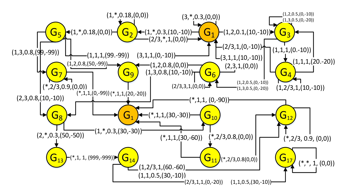
We find three pairs of states which are probabilistic bisimilar: s13∼s15s_{13}\sim s_{15}, s14∼s16s_{14}\sim s_{16} and s17∼s18s_{17}\sim s_{18}. Figure 4 shows the ConTS of case study.
Refer to caption
Figure 4: ConTS of Example

4.2 Analyzing NES/SOS for Case study

We implement the algorithms using Java in Eclipse development environment on machine with 3.4GHz Inter(R) Core(TM) i72.99G RAM. We get two Nash Equlibrium Strategies and one Social Optimal strategy for our case study, shown in Figure 5, 6, 7 respectively.

Refer to caption
Figure 5: Nash Equilibrium strategy 1
Refer to caption
Figure 6: Nash Equilibrium strategy 2
Refer to caption
Figure 7: Social Optimal strategy

4.3 Evaluation

We compare our results with those obtained in [12] by game-theoretic approach:
(1) We filter the invalid Nash Equilibrium strategy from the results in [12]. We filter the action pair (ϕ\phi, R​e​m​o​v​e​_Remove\_ Sniffer​_\textit{Sniffer}\_ D​e​t​e​c​o​rDetecor) at state s3s_{3} and the action pair (I​n​s​t​r​a​l​l​_Instrall\_ Sniffer​_\textit{Sniffer}\_ D​e​t​e​c​t​o​rDetector, R​e​m​o​v​e​_Remove\_Compromised_account_ restart_ftpd)) at s6s_{6} which obtained in the second Nash Equilibrium strategy in [12] but have no practical state transition.
(2) We minimize the state space by probabilistic bisimulation while [12] focuses on the whole state set. Time consumed to compute Nash Equilibrium strategy and Social Optimal strategy for this example with our approach is shown in Table 2. Although it is incomparable with the time consumed in [12] because of evaluating on different machine models, our approach should be faster theoretically.

ComModel Nash Equilibrium Social Optimal
Creation strategy strategy
2.8s 3.7s 1.4s
Table 2: Time consumed for example with our approach

5 Conclusion

We proposed a probabilistic value-passing CCS (PVCCS) approach for modeling and analyzing a typical network security scenario with one attacker and one defender which is usually modeled by perfect and complete information game. Extention of this method might provide uniform framework for modelling and analyzing network security scenarios which are usually modeled via different games. We designed two algorithms for computing Nash Equilibrium strategy and Social Optimal strategy based on this PVCCS approach and on graph-theoretic methods. Advantages of these algorithms are also discussed.

References

  • [1] M. Abadi and A. D. Gordon. A calculus for cryptographic protocols: The spi calculus. In The 4th ACM Conf on Computer and Communications Security, 1997.
  • [2] J. Bergstra and J. Klop. Verification of an alternating bit protocol by means of process algebra. Technical report, Centrum voor Wiskunde en Informatica, 1984.
  • [3] K. Chatzikokolakis, D. Gebler, C. Palamidessi, and L. Xu. Generalized bisimulation metrics. In Proc. of CONCUR, volume 8704, pages 32–46, 2014.
  • [4] Y. Deng. Semantics of probabilistic process–An operational approach. Springer, 2014.
  • [5] R. Diestel. Graph Theory. Springer-Verlag, 3 edition, 2005.
  • [6] D. Easley and J. Kleinberg. Networks, Crowds, and Markets:Reasoning about a Highly Connected World. Cambridge University Press, 2010.
  • [7] J. C. HARSANYI. Games with incomplete information played by bayesian players, i-iii. Management Science, 14(3), 1967.
  • [8] E. M. Jean Tirole. Markov perfect equilibrium. Journal of Economic Theory, 2001.
  • [9] J. Jormakka and J. Molsa. Modelling information warfare as a game. In Journal of Information Warfare, volume 4 of 2, 2005.
  • [10] a. T. B. K. C. Nguyen, T. Alpcan. Stochastic games for security in networks with interdependent nodes. In Proc. of Intl. Conf. on Game Theory for Networks (GameNets), 2009.
  • [11] X. Liang and Y. Xiao. Game theory for network security. In IEEE Communications Surveys and amp Tutorials, 2013.
  • [12] K. Lye and J. Wing. Game strategies in network security. In Proceedings of the Foundations of Computer Security, 2005.
  • [13] R. Milner. Communication and Cocurrency. Prentice Hall International Ltd, 1989.
  • [14] M. J. Osborne. An Introduction to Game Theory. Oxford University Press., 2000.
  • [15] M. J. Osborne and A. Rubinstein. A course in Game Theory. MIT Press, 1994.
  • [16] A. Patcha and J. Park. A game theoretic apporach to modeling intrusion detection in mobile ad hoc networks. In Proceedings of the 2004 IEEE workshop on Information Assurance and Security, 2004.
  • [17] S. Roy and C. Ellis. A survey of game theory as applied to network security. In 43r​d43^{rd} Hawaii International Conference on System Sciences, 2010.
  • [18] D. Sangiorgi. An introduction to Bisimulation and Coinduction. Springer, 2007.
  • [19] I. M. Serge Abiteboul and P. Rigaux. Web data management. Cambridge University Press, 2011.
  • [20] L. Shapley. Stochastic Games. Princeton University press, 1953.
  • [21] P. Syverson. A different look at secure distributed computation. In Proc. 10th IEEE Computer Security Foundations Workshop, 1997.
  • [22] R. van Glabbeek, S. A. Smolka, B. Steffen, and C. M. Tofts. Reactive,generative,and stratified models of probabilistic processes. In Information and Computation, 1995.
  • [23] J. V. D. Wal. Stochastic dynamic programming. In Mathematical Centre Tracts 139. Morgan Kaufmann, 1981.
  • [24] C. Xiaolin, T. Xiaobin, Z. Yong, and X. Hongsheng. A markov game theory-based risk assessment model for network information systems. In International conference on computer science and software engineering, 2008.

Appendix A Proofs of Theorems

Proof of Theorem 3.1

Proof A.1.

As vertex set VV is finite, then any infinite execution πi\pi_{\textit{i}} of GiG_{\textit{i}} is in form of Gi​ei1​G1​…​(Gk​…​G(k+m)​e(k+m)k​Gk)G_{\textit{i}}e_{\textit{i1}}G_{\textit{1}}...(G_{\textit{k}}...G_{\textit{(k+m)}}e_{\textit{(k+m)k}}G_{\textit{k}}) which means ending with a cycle starting with GkG_{\textit{k}}, and mm is the number of vertex on this cycle except GkG_{\textit{k}}, then we have

P​Fa​(πi)\displaystyle PF^{a}(\pi_{\textit{i}}) =LWeiPa​(ei1)+β⋅P​Fa​(πi​[1])\displaystyle=L^{a}_{\textit{WeiP}}(e_{\textit{i1}})+\beta\cdot PF^{a}(\pi_{\textit{i}}[1])
=LWeiPa​(ei1)+…+βk⋅P​Fa​(πi​[k])\displaystyle=L^{a}_{\textit{WeiP}}(e_{\textit{i1}})+...+\beta^{k}\cdot PF^{a}(\pi_{\textit{i}}[k])
=A+βk⋅P​Fa​(πi​[k])\displaystyle=A+\beta^{k}\cdot PF^{a}(\pi_{\textit{i}}[k])
w​h​e​r​e​A\displaystyle where~A =LWeiPa​(ei1)+…+βk−1⋅LWeiPa​(e(k-1)k)\displaystyle=L^{a}_{\textit{WeiP}}(e_{\textit{i1}})+...+\beta^{k-1}\cdot L^{a}_{\textit{WeiP}}(e_{\textit{(k-1)k}})
P​Fa​(πi​[k])\displaystyle PF^{a}(\pi_{\textit{i}}[k]) =LWeiPa​(ek(k+1))+…+βm⋅LWeiPa​(e(k+m)k)\displaystyle=L^{a}_{\textit{WeiP}}(e_{\textit{k(k+1)}})+...+\beta^{m}\cdot L^{a}_{\textit{WeiP}}(e_{\textit{(k+m)k}})
+βm+1⋅B+β2​m+2⋅B+…\displaystyle+\beta^{m+1}\cdot B+\beta^{2m+2}\cdot B+...
=(B⋅1−β(m+1)​h1−β(m+1))h→∞\displaystyle=(B\cdot\frac{1-\beta^{(m+1)h}}{1-\beta^{(m+1)}})_{h\rightarrow\infty}
w​h​e​r​e​B\displaystyle where~B =LWeiPa​(ek(k+1))+…+βm⋅LWeiPa​(e(k+m)k)\displaystyle=L^{a}_{\textit{WeiP}}(e_{\textit{k(k+1)}})+...+\beta^{m}\cdot L^{a}_{\textit{WeiP}}(e_{\textit{(k+m)k}})
limh→∞​P​Fa​(πi)\displaystyle\underset{h\rightarrow\infty}{\lim}PF^{a}(\pi_{\textit{i}}) =limh→∞​(A+βk​(B⋅1−β(m+1)​h1−β(m+1)))\displaystyle=\underset{h\rightarrow\infty}{\lim}(A+\beta^{k}(B\cdot\frac{1-\beta^{(m+1)h}}{1-\beta^{(m+1)}}))
=A+βk⋅B⋅limh→∞​(1−β(m+1)​h1−β(m+1))\displaystyle=A+\beta^{k}\cdot B\cdot\underset{h\rightarrow\infty}{\lim}(\frac{1-\beta^{(m+1)h}}{1-\beta^{(m+1)}})
=A+B⋅βk1−β(m+1)\displaystyle=A+B\cdot\frac{\beta^{k}}{1-\beta^{(m+1)}}

Proof of Lemma 3.1

Proof A.2.

Assuming without loss of generality, σk​(Gi)=(Lk​(e1)a,Lk​(e1)d)\sigma_{k}(G_{\textit{i}})=(L_{k}(e_{1})^{a},L_{k}(e_{1})^{d}) and T​σk​(Gi)=(Lk+1​(e2)a,Lk+1​(e2)d)T\sigma_{k}(G_{\textit{i}})=(L_{k+1}(e_{2})^{a},L_{k+1}(e_{2})^{d}), where e1e_{1}, e2∈E⁡(Gi)e_{2}\in E(G_{\textit{i}}). Let Lka​(e1)=aL_{k}^{a}(e_{1})=a, Lka​(e2)=bL_{k}^{a}(e_{2})=b, Lk+1a​(e1)=a′L_{k+1}^{a}(e_{1})=a^{\prime} and Lk+1a​(e2)=b′L_{k+1}^{a}(e_{2})=b^{\prime}, where aa, a′a^{\prime}, bb, b′b^{\prime} are positive number.
case 1: LActa​(e1)=LActa​(e2)L_{\textit{Act}}^{a}(e_{1})=L_{\textit{Act}}^{a}(e_{2})
According to the rules of BackInd(), we have a<ba<b and b′<a′b^{\prime}<a^{\prime}. If the first inequality in lemma doesn’t hold, then we have ∣a−b′∣>∣a−a′∣\mid a-b^{\prime}\mid>\mid a-a^{\prime}\mid and ∣a−b′∣>∣b−b′∣\mid a-b^{\prime}\mid>\mid b-b^{\prime}\mid, then we get (b′−a′)​(b′+a′)>2​a​(b′−a′)(b^{\prime}-a^{\prime})(b^{\prime}+a^{\prime})>2a(b^{\prime}-a^{\prime}) and (a−b)​(a+b)>2​b′​(a−b)(a-b)(a+b)>2b^{\prime}(a-b) which deduce a−b>a′−b′a-b>a^{\prime}-b^{\prime}, contradiction.
case 2: LActa​(e1)≠LActa​(e2)L_{\textit{Act}}^{a}(e_{1})\neq L_{\textit{Act}}^{a}(e_{2})
Let us define two conditions:
Cond 1: on kth iteration, e2e_{2} is kept by step (2) of BackInd().
Cond 2: on (k+1)th iteration, e1e_{1} is kept by step (2) of BackInd().
There are four subcases to be considered:
case 2.1: both Cond 1 and Cond 2
According to the rules of BackInd(), we have a>ba>b and b′>a′b^{\prime}>a^{\prime}. If ∣a−b′∣>∣a−a′∣\mid a-b^{\prime}\mid>\mid a-a^{\prime}\mid and ∣a−b′∣>∣b−b′∣\mid a-b^{\prime}\mid>\mid b-b^{\prime}\mid, then we get b−a>b′−a′b-a>b^{\prime}-a^{\prime}, contradiction.
case 2.2: not Cond 2 but Cond 1
According to the rules of BackInd(), ∃e′\exists e^{\prime} with LA​c​ta​(e′)=LA​c​ta​(e1)L_{Act}^{a}(e^{\prime})=L_{Act}^{a}(e_{1}). Assuming Lka​(e′)=cL_{k}^{a}(e^{\prime})=c and Lk+1a​(e′)=c′L_{k+1}^{a}(e^{\prime})=c^{\prime}, then we have c>a>bc>a>b, a′>c′a^{\prime}>c^{\prime} and b′>c′b^{\prime}>c^{\prime}. If ∣a−b′∣>∣a−a′∣\mid a-b^{\prime}\mid>\mid a-a^{\prime}\mid and ∣a−b′∣>∣b−b′∣\mid a-b^{\prime}\mid>\mid b-b^{\prime}\mid, then we have (b′−a′)​(b′+a′)>2​a​(b′−a′)(b^{\prime}-a^{\prime})(b^{\prime}+a^{\prime})>2a(b^{\prime}-a^{\prime}) and a+b>2​b′a+b>2b^{\prime}. If b′>a′>c′b^{\prime}>a^{\prime}>c^{\prime}, it is trivial to get contradiction; If c′<b′<a′c^{\prime}<b^{\prime}<a^{\prime}, then we have 2​b′<b′+a′<2​a2b^{\prime}<b^{\prime}+a^{\prime}<2a and 2​c>a+b>2​b′>2​c′2c>a+b>2b^{\prime}>2c^{\prime}, then we have b′<ab^{\prime}<a and c>c′c>c^{\prime}. If ∣a−b′∣>∣c−c′∣\mid a-b^{\prime}\mid>\mid c-c^{\prime}\mid, then we have a−c>b′−c′a-c>b^{\prime}-c^{\prime}, contradiction; If b′=a′b^{\prime}=a^{\prime}, contradiction.
case 2.3: not Cond 1 but Cond 2
According to the rules of BackInd(), ∃e′\exists e^{\prime} with LA​c​ta​(e′)=LA​c​ta​(e2)L_{Act}^{a}(e^{\prime})=L_{Act}^{a}(e_{2}). proof is similar to case 2.2.
case 2.4: neither Cond 1 nor Cond 2
According to the rules of BackInd(), ∃e′,e′′\exists e^{\prime},e^{\prime\prime} with LA​c​ta​(e′)=LA​c​ta​(e1)L_{Act}^{a}(e^{\prime})=L_{Act}^{a}(e_{1}) and LA​c​ta​(e′′)=LA​c​ta​(e2)L_{Act}^{a}(e^{\prime\prime})=L_{Act}^{a}(e_{2}). Assuming Lka​(e′)=cL_{k}^{a}(e^{\prime})=c and Lk+1a​(e′)=c′L_{k+1}^{a}(e^{\prime})=c^{\prime},Lka​(e′′)=dL_{k}^{a}(e^{\prime\prime})=d and Lk+1a​(e′′)=d′L_{k+1}^{a}(e^{\prime\prime})=d^{\prime}, then we have d<a<cd<a<c, d<bd<b, a′>c′a^{\prime}>c^{\prime} and c′<b′<d′c^{\prime}<b^{\prime}<d^{\prime}. If ∣a−b′∣>∣a−a′∣\mid a-b^{\prime}\mid>\mid a-a^{\prime}\mid and ∣a−b′∣>∣b−b′∣\mid a-b^{\prime}\mid>\mid b-b^{\prime}\mid, then we have (b′−a′)​(b′+a′)>2​a​(b′−a′)(b^{\prime}-a^{\prime})(b^{\prime}+a^{\prime})>2a(b^{\prime}-a^{\prime}) and (a−b)​(a+b)>2​b′​(a−b)(a-b)(a+b)>2b^{\prime}(a-b). If a>ba>b and a′>b′a^{\prime}>b^{\prime}, then we have c′<cc^{\prime}<c and a>b′a>b^{\prime}, and if ∣a−b′∣>∣c−c′∣\mid a-b^{\prime}\mid>\mid c-c^{\prime}\mid, then we a−c>b′−c′a-c>b^{\prime}-c^{\prime}, contradiction; If a<ba<b and a′>b′a^{\prime}>b^{\prime} or a>ba>b and a′<b′a^{\prime}<b^{\prime}, it is trivial to get contradiction; If a<ba<b and a′<b′a^{\prime}<b^{\prime}, then we get d′>dd^{\prime}>d and a<b′a<b^{\prime}, and if ∣a−b′∣>∣d−d′∣\mid a-b^{\prime}\mid>\mid d-d^{\prime}\mid, then we get b′−d′>a−db^{\prime}-d^{\prime}>a-d, contradiction.
Proof for second inequality is similar. We skip the details.

Proof for Theorem 3.3.

Proof A.3.

We need to prove two issues:
1.
NESinLeave(DD) is terminated.
The way to prove termination of
NESinLeave(DD) is to prove ∃k\exists k that after kth iteration, ∀Gi,P​pk​(Gi)=P​pk+1​(Gi)\forall G_{\textit{i}},~Pp_{\textit{k}}(G_{\textit{i}})=Pp_{\textit{k+1}}(G_{\textit{i}}). According to Lemma 3.2, trivial;
2. The result of
NESinLeave(DD) is NES of DD. ∀Gi∈𝒱⁡(D)\forall G_{i}\in\mathcal{V}(D), assuming πi\pi_{\textit{i}} whose first edge is ee is the execution of GiG_{\textit{i}} based on the result obtained by NESinLeave(DD), we need to prove πie\pi_{\textit{i}}^{e} is NEE of GiG_{\textit{i}} coinductively. As πie\pi_{\textit{i}}^{e} is ended by a cycle, we just need to prove any e′e^{\prime} on πie\pi_{\textit{i}}^{e}, e′∈E⁡(Gj)e^{\prime}\in E(G_{\textit{j}}), is the first edge of NEE of GjG_{\textit{j}}. We prove edge ee of GiG_{\textit{i}} as example. If πie\pi_{\textit{i}}^{e} is not NEE of GiG_{\textit{i}}, according to the definition of NEE, there exists πie′\pi_{\textit{i}}^{e^{\prime}} satisfying: (1) P​Fd​(πie′)>P​Fd​(πie)PF^{d}(\pi_{\textit{i}}^{e^{\prime}})>PF^{d}(\pi_{\textit{i}}^{e}) where LActa​(e′)=LActa​(e)L_{\textit{Act}}^{a}(e^{\prime})=L_{\textit{Act}}^{a}(e) or (2) P​Fa​(πie′)>P​Fa​(πie)PF^{a}(\pi_{\textit{i}}^{e^{\prime}})>PF^{a}(\pi_{\textit{i}}^{e}) where e′=arg⁡maxe′′∈Ea​(Gi,e′)​P​Fd​(πie′′)e^{\prime}=\arg\underset{e^{\prime\prime}\in E^{a}(G_{\textit{i}},e^{\prime})}{\max}PF^{d}(\pi_{\textit{i}}^{e^{\prime\prime}}), and both of them are contradicted with the rules in BackInd().

Appendix B Tables of case study

To make paper self-contained, we list the data related in example created in [12].

State number State name
1 N​o​r​m​a​l​_​o​p​e​r​a​t​i​o​nNormal\_operation
2 H​t​t​p​d​_​a​t​t​a​c​k​e​dHttpd\_attacked
3 F​t​p​_​a​t​t​a​c​k​e​dFtp\_attacked
4 F​t​p​d​_​a​t​t​a​c​k​e​dd​e​t​e​c​t​o​rFtpd\_attacked_{d}etector
5 H​t​t​p​d​_​h​a​c​k​e​dHttpd\_hacked
6 F​t​p​d​_​h​a​c​k​e​dFtpd\_hacked
7 W​e​b​s​i​t​e​_​d​e​f​a​c​e​dWebsite\_defaced
8 W​e​b​s​e​v​e​r​_​s​n​i​f​f​e​rWebsever\_sniffer
9 W​e​b​s​e​v​e​r​_​s​n​i​f​f​e​r​_​d​e​t​e​c​t​o​rWebsever\_sniffer\_detector
10 W​e​b​s​e​v​e​r​_​D​O​S​_​1Websever\_DOS\_1
11 W​e​b​s​e​v​e​r​_​D​O​S​_​2Websever\_DOS\_2
12 N​e​t​w​o​r​k​_​s​h​u​t​d​o​w​nNetwork\_shutdown
13 F​i​l​e​s​e​v​e​r​_​h​a​c​k​e​dFilesever\_hacked
14 F​i​l​e​s​e​v​e​r​_​d​a​t​a​_​s​t​o​l​e​nFilesever\_data\_stolen
15 W​o​r​k​s​t​a​t​i​o​n​_​h​a​c​k​e​dWorkstation\_hacked
16 W​o​r​k​s​t​a​t​i​o​n​_​d​a​t​a​_​s​t​o​l​e​n​_​1Workstation\_data\_stolen\_1
17 F​i​l​e​s​e​v​e​r​_​d​a​t​a​_​s​t​o​l​e​nFilesever\_data\_stolen
18 W​o​r​k​s​t​a​t​i​o​n​_​d​a​t​a​_​s​t​o​l​e​n​_​2Workstation\_data\_stolen\_2
Table 3: Network state
S​t​a​t​e​n​o.\State~no.\backslash 1 2 3
Action no.
1 ϕ\phi ϕ\phi ϕ\phi
2 ϕ\phi ϕ\phi ϕ\phi
3 I​n​s​t​a​l​l​_​S​n​i​f​f​e​r​_Install\_Sniffer\_ ϕ\phi ϕ\phi
D​e​t​c​t​o​rDetctor
4 R​e​m​o​v​e​_​S​n​i​f​f​e​r​_Remove\_Sniffer\_ ϕ\phi ϕ\phi
D​e​t​c​t​o​rDetctor
5 R​e​m​o​v​e​_​C​o​m​p​r​o​m​i​s​e​d​_Remove\_Compromised\_ I​n​s​t​a​l​l​_​s​n​i​f​f​e​r​_Install\_sniffer\_ ϕ\phi
a​c​c​o​u​n​t​_​r​e​s​t​a​r​t​_​h​t​t​p​daccount\_restart\_httpd d​e​t​e​c​t​o​rdetector
6 R​e​m​o​v​e​_​C​o​m​p​r​o​m​i​s​e​d​_Remove\_Compromised\_ I​n​s​t​a​l​l​_​s​n​i​f​f​e​r​_Install\_sniffer\_ ϕ\phi
a​c​c​o​u​n​t​_​r​e​s​t​a​r​t​_​f​t​p​daccount\_restart\_ftpd d​e​t​e​c​t​o​rdetector
7 R​e​s​t​o​r​e​_​w​e​b​s​i​t​e​_​r​e​m​o​v​e​_Restore\_website\_remove\_ ϕ\phi ϕ\phi
c​o​m​p​r​o​m​i​s​e​d​_​a​c​c​o​u​n​tcompromised\_account
8 ϕ\phi ϕ\phi ϕ\phi
9 R​e​m​o​v​e​_​s​n​i​f​f​e​r​_​a​n​d​_Remove\_sniffer\_and\_ ϕ\phi ϕ\phi
C​o​m​p​r​o​m​i​s​e​d​_​a​c​c​o​u​n​tCompromised\_account
10 R​e​m​o​v​e​_​v​i​r​u​s​_​a​n​d​_Remove\_virus\_and\_ ϕ\phi ϕ\phi
C​o​m​p​r​o​m​i​s​e​d​_​a​c​c​o​u​n​tCompromised\_account
11 R​e​m​o​v​e​_​v​i​r​u​s​_​a​n​d​_Remove\_virus\_and\_ ϕ\phi ϕ\phi
C​o​m​p​r​o​m​i​s​e​d​_​a​c​c​o​u​nCompromised\_accoun
12 R​e​m​o​v​e​_​v​i​r​u​s​_​a​n​d​_Remove\_virus\_and\_ ϕ\phi ϕ\phi
C​o​m​p​r​o​m​i​s​e​d​_​a​c​c​o​u​n​tCompromised\_account
13 ϕ\phi ϕ\phi ϕ\phi
14 R​e​m​o​v​e​_​s​n​i​f​f​e​r​_​a​n​dRemove\_sniffer\_and ϕ\phi ϕ\phi
_​C​o​m​p​r​o​m​i​s​e​d​_​a​c​c​o​u​n​t\_Compromised\_account
15 ϕ\phi ϕ\phi ϕ\phi
16 R​e​m​o​v​e​_​s​n​i​f​f​e​r​_​a​n​dRemove\_sniffer\_and ϕ\phi ϕ\phi
_​C​o​m​p​r​o​m​i​s​e​d​_​a​c​c​o​u​n​t\_Compromised\_account
17 ϕ\phi ϕ\phi ϕ\phi
18 ϕ\phi ϕ\phi ϕ\phi
Table 4: Defender’s action set
S​t​a​t​e​n​o.\State~no.\backslash 1 2 3
Action no.
1 A​t​t​a​c​k​_​h​t​t​p​dAttack\_httpd A​t​t​a​c​kf​t​p​dAttack_{f}tpd ϕ\phi
2 C​o​n​t​i​n​u​e​_Continue\_ ϕ\phi ϕ\phi
a​t​t​a​c​k​i​n​gattacking
3 C​o​n​t​i​n​u​e​_Continue\_ ϕ\phi ϕ\phi
a​t​t​a​c​k​i​n​gattacking
4 C​o​n​t​i​n​u​e​_Continue\_ ϕ\phi ϕ\phi
a​t​t​a​c​k​i​n​gattacking
5 D​e​f​a​c​e​_Deface\_ I​n​s​t​a​l​l​_Install\_ ϕ\phi
w​e​b​s​i​t​ewebsite s​n​i​f​f​e​rsniffer
6 I​n​s​t​a​l​l​_Install\_ ϕ\phi ϕ\phi
s​n​i​f​f​e​rsniffer
7 ϕ\phi ϕ\phi ϕ\phi
8 R​u​n​_​D​O​SRun\_DOS C​r​a​c​k​_​f​i​l​e​s​e​r​v​e​r​_Crack\_fileserver\_ C​r​a​c​k​_​w​o​r​k​s​t​a​t​i​o​nCrack\_workstation
_​v​i​r​u​s\_virus r​o​o​t​_​p​a​s​s​w​o​r​droot\_password _​r​o​o​t​_​p​a​s​s​w​o​r​d\_root\_password
9 ϕ\phi ϕ\phi ϕ\phi
10 ϕ\phi ϕ\phi ϕ\phi
11 ϕ\phi ϕ\phi ϕ\phi
12 ϕ\phi ϕ\phi ϕ\phi
13 C​a​p​t​u​r​eCapture ϕ\phi ϕ\phi
_​d​a​t​a\_data
14 S​h​u​t​d​o​w​nShutdown ϕ\phi ϕ\phi
_​n​e​t​w​o​r​k\_network
15 C​a​p​t​u​r​eCapture ϕ\phi ϕ\phi
_​d​a​t​a\_data
16 S​h​u​t​d​o​w​nShutdown ϕ\phi ϕ\phi
_​n​e​t​w​o​r​k\_network
17 ϕ\phi ϕ\phi ϕ\phi
18 ϕ\phi ϕ\phi ϕ\phi
Table 5: Attacker’s action set
R1​(1)=[101010101010000]R^{1}(1)=\begin{bmatrix}10&10&10\\ 10&10&10\\ 0&0&0\end{bmatrix} R2​(1)=−R1​(1)R^{2}(1)=-R^{1}(1)
R1​(2)=[000000000]R^{1}(2)=\begin{bmatrix}0&0&0\\ 0&0&0\\ 0&0&0\end{bmatrix} R2​(2)=R1​(2)R^{2}(2)=R^{1}(2)
R1​(3)=[000000000]R^{1}(3)=\begin{bmatrix}0&0&0\\ 0&0&0\\ 0&0&0\end{bmatrix} R2​(3)=[−10−10−20−10−100−10−100]R^{2}(3)=\begin{bmatrix}-10&-10&-20\\ -10&-10&0\\ -10&-10&0\end{bmatrix}
R1​(4)=[201010000000]R^{1}(4)=\begin{bmatrix}20&10&10\\ 0&0&0\\ 0&0&0\end{bmatrix} R2​(4)=[−20−10−10−1000−1000]R^{2}(4)=\begin{bmatrix}-20&-10&-10\\ -10&0&0\\ -10&0&0\end{bmatrix}
R1​(5)=[995099100100100]R^{1}(5)=\begin{bmatrix}99&50&99\\ 10&0&10\\ 0&10&0\end{bmatrix} R2​(5)=[−99−99−991010−10−10−100]R^{2}(5)=\begin{bmatrix}-99&-99&-99\\ 10&10&-10\\ -10&-10&0\end{bmatrix}
R1​(6)=[001010001000]R^{1}(6)=\begin{bmatrix}0&0&10\\ 10&0&0\\ 10&0&0\end{bmatrix} R2​(6)=−R1​(6)R^{2}(6)=-R^{1}(6)
R1​(7)=[000000000]R^{1}(7)=\begin{bmatrix}0&0&0\\ 0&0&0\\ 0&0&0\end{bmatrix} R2​(7)=[−9900−9900−9900]R^{2}(7)=\begin{bmatrix}-99&0&0\\ -99&0&0\\ -99&0&0\end{bmatrix}
R1​(8)=[303030505050505050]R^{1}(8)=\begin{bmatrix}30&30&30\\ 50&50&50\\ 50&50&50\end{bmatrix} R2​(8)=−R1​(8)R^{2}(8)=-R^{1}(8)
R1​(9)=[−2000−2000−2000]R^{1}(9)=\begin{bmatrix}-20&0&0\\ -20&0&0\\ -20&0&0\end{bmatrix} R2​(9)=R1​(9)R^{2}(9)=R^{1}(9)
R1​(10)=[300030003000]R^{1}(10)=\begin{bmatrix}30&0&0\\ 30&0&0\\ 30&0&0\end{bmatrix} R2​(10)=−R1​(10)R^{2}(10)=-R^{1}(10)
R1​(11)=[300030003000]R^{1}(11)=\begin{bmatrix}30&0&0\\ 30&0&0\\ 30&0&0\end{bmatrix} R2​(11)=[−6000−6000−6000]R^{2}(11)=\begin{bmatrix}-60&0&0\\ -60&0&0\\ -60&0&0\end{bmatrix}
R1​(12)=[000000000]R^{1}(12)=\begin{bmatrix}0&0&0\\ 0&0&0\\ 0&0&0\end{bmatrix} R2​(12)=[−9000−9000−9000]R^{2}(12)=\begin{bmatrix}-90&0&0\\ -90&0&0\\ -90&0&0\end{bmatrix}
R1​(13)=[999009990099900]R^{1}(13)=\begin{bmatrix}999&0&0\\ 999&0&0\\ 999&0&0\end{bmatrix} R2​(13)=−R1​(13)R^{2}(13)=-R^{1}(13)
R1​(14)=[306060000000]R^{1}(14)=\begin{bmatrix}30&60&60\\ 0&0&0\\ 0&0&0\end{bmatrix} R2​(14)=[−10−60−60−2000−2000]R^{2}(14)=\begin{bmatrix}-10&-60&-60\\ -20&0&0\\ -20&0&0\end{bmatrix}
R1​(15)=[999009990099900]R^{1}(15)=\begin{bmatrix}999&0&0\\ 999&0&0\\ 999&0&0\end{bmatrix} R2​(15)=−R1​(13)R^{2}(15)=-R^{1}(13)
R1​(16)=[306060000000]R^{1}(16)=\begin{bmatrix}30&60&60\\ 0&0&0\\ 0&0&0\end{bmatrix} R2​(16)=[−10−60−60−2000−2000]R^{2}(16)=\begin{bmatrix}-10&-60&-60\\ -20&0&0\\ -20&0&0\end{bmatrix}
R1​(17)=[000000000]R^{1}(17)=\begin{bmatrix}0&0&0\\ 0&0&0\\ 0&0&0\end{bmatrix} R2​(17)=R1​(17)R^{2}(17)=R^{1}(17)
R1​(18)=[000000000]R^{1}(18)=\begin{bmatrix}0&0&0\\ 0&0&0\\ 0&0&0\end{bmatrix} R2​(18)=R1​(18)R^{2}(18)=R^{1}(18)
Table 6: Immediate payoff to Attacker and Defender
𝐒𝐭𝐚𝐭𝐞​𝟏\bf State~1 𝐒𝐭𝐚𝐭𝐞​𝟐\bf State~2 𝐒𝐭𝐚𝐭𝐞​𝟑\bf State~3
p(2|1,1,⋅)=1/3p(2|1,1,\cdot)=1/3 p(2|2,1,⋅)=0.5/3p(2|2,1,\cdot)=0.5/3 p⁡(3|3,1,2)=0.5p(3|3,1,2)=0.5
p⁡(3|1,1,2)=1/3p(3|1,1,2)=1/3 p(5|2,1,⋅)=0.5/3p(5|2,1,\cdot)=0.5/3 p⁡(3|3,1,3)=0.5p(3|3,1,3)=0.5
p(1|1,3,⋅)=1/3p(1|1,3,\cdot)=1/3 p(1|2,2,⋅)=1p(1|2,2,\cdot)=1 p⁡(6|3,1,2)=0.5p(6|3,1,2)=0.5
p(1|2,3,⋅)=1p(1|2,3,\cdot)=1 p⁡(6|3,1,3)=0.5p(6|3,1,3)=0.5
p⁡(4|3,1,1)=1p(4|3,1,1)=1
𝐒𝐭𝐚𝐭𝐞​𝟒\bf State~4 𝐒𝐭𝐚𝐭𝐞​𝟓\bf State~5 𝐒𝐭𝐚𝐭𝐞​𝟔\bf State~6
p⁡(1|4,2,1)=1p(1|4,2,1)=1 p⁡(7|5,1,3)=0.8p(7|5,1,3)=0.8 p⁡(8|6,1,3)=0.8p(8|6,1,3)=0.8
p⁡(1|4,3,1)=1p(1|4,3,1)=1 p⁡(8|5,2,3)=0.8p(8|5,2,3)=0.8 p⁡(9|6,1,2)=0.8p(9|6,1,2)=0.8
p⁡(3|4,1,1)=1p(3|4,1,1)=1 p⁡(9|5,1,2)=0.8p(9|5,1,2)=0.8 p⁡(1|6,2,3)=1p(1|6,2,3)=1
p⁡(4|4,1,2)=1p(4|4,1,2)=1 p⁡(1|5,3,1)=1p(1|5,3,1)=1 p⁡(1|6,3,1)=1p(1|6,3,1)=1
p⁡(4|4,1,3)=1p(4|4,1,3)=1 p⁡(1|5,1,1)=1p(1|5,1,1)=1 p⁡(6|6,2,3)=1p(6|6,2,3)=1
p⁡(6|6,3,3)=1p(6|6,3,3)=1
𝐒𝐭𝐚𝐭𝐞​𝟕\bf State~7 𝐒𝐭𝐚𝐭𝐞​𝟖\bf State~8 𝐒𝐭𝐚𝐭𝐞​𝟗\bf State~9
p(1|7,⋅,1)=1p(1|7,\cdot,1)=1 p(10|8,1,⋅)=1/3p(10|8,1,\cdot)=1/3 p(1|9,⋅,1)=1p(1|9,\cdot,1)=1
p(7|7,⋅,2)=0.9p(7|7,\cdot,2)=0.9 p(13|8,2,⋅)=0.3p(13|8,2,\cdot)=0.3
p(7|7,⋅,3)=0.9p(7|7,\cdot,3)=0.9 p(15|8,3,⋅)=0.3p(15|8,3,\cdot)=0.3
𝐒𝐭𝐚𝐭𝐞​𝟏𝟎\bf State~10 𝐒𝐭𝐚𝐭𝐞​𝟏𝟏\bf State~11 𝐒𝐭𝐚𝐭𝐞​𝟏𝟐\bf State~12
p(1|10,⋅,1)=1p(1|10,\cdot,1)=1 p(1|11,⋅,1)=1p(1|11,\cdot,1)=1 p(1|12,1,⋅)=1p(1|12,1,\cdot)=1
p(11|10,⋅,2)=0.8p(11|10,\cdot,2)=0.8 p(12|11,⋅,2)=0.8p(12|11,\cdot,2)=0.8 p(12|12,⋅,2)=0.9p(12|12,\cdot,2)=0.9
p(11|10,⋅,3)=0.8p(11|10,\cdot,3)=0.8 p(12|11,⋅,3)=0.8p(12|11,\cdot,3)=0.8 p(12|12,⋅,3)=0.9p(12|12,\cdot,3)=0.9
𝐒𝐭𝐚𝐭𝐞​𝟏𝟑\bf State~13 𝐒𝐭𝐚𝐭𝐞​𝟏𝟒\bf State~14 𝐒𝐭𝐚𝐭𝐞​𝟏𝟓\bf State~15
p(14|13,1,⋅)=1p(14|13,1,\cdot)=1 p⁡(12|14,1,2)=1p(12|14,1,2)=1 p(16|15,1,⋅)=1p(16|15,1,\cdot)=1
p⁡(12|14,1,3)=1p(12|14,1,3)=1
p⁡(17|14,2,1)=1p(17|14,2,1)=1
p⁡(17|14,3,1)=1p(17|14,3,1)=1
p⁡(12|14,1,1)=0.5p(12|14,1,1)=0.5
p⁡(17|14,1,1)=0.5p(17|14,1,1)=0.5
𝐒𝐭𝐚𝐭𝐞​𝟏𝟔\bf State~16 𝐒𝐭𝐚𝐭𝐞​𝟏𝟕\bf State~17 𝐒𝐭𝐚𝐭𝐞​𝟏𝟖\bf State~18
p⁡(12|16,1,2)=1p(12|16,1,2)=1 p(17|17,⋅,⋅)=0.9p(17|17,\cdot,\cdot)=0.9 p(18|18,⋅,⋅)=0.9p(18|18,\cdot,\cdot)=0.9
p⁡(12|16,1,3)=1p(12|16,1,3)=1
p⁡(18|16,2,1)=1p(18|16,2,1)=1
p⁡(18|16,3,1)=1p(18|16,3,1)=1
p⁡(12|16,1,1)=0.5p(12|16,1,1)=0.5
p⁡(18|16,1,1)=0.5p(18|16,1,1)=0.5
Table 7: State transition probabilities


Appendix C Notation Index

A​b​s,5Abs,~5 NESinNonLeave⁡(),7\rm{NESinNonLeave()},~7
AlgNES⁡(),5\rm{AlgNES()},~5 P​Fa​(πi),4PF^{a}(\pi_{\textit{i}}),~4
AlgSOS⁡(),5\rm{AlgSOS()},~5 P​Fd​(πi),4PF^{d}(\pi_{\textit{i}}),~4
BackInd⁡(),6\rm{BackInd()},~6 P​pn​(Gi),6Pp_{n}(G_{\textit{i}}),~6
ComModel,3\textbf{ComModel},~3 P​sn​(Gi),6Ps_{n}(G_{\textit{i}}),~6
ConTS,4\rm{ConTS},~4 PrePro⁡(),7\rm{PrePro()},~7
D,5D,~5 PreProS⁡(),7\rm{PreProS()},~7
e​x​e​c​u​t​i​o​n,4execution,~4 PVCCS​R,2\rm{PVCCS}\textsubscript{R},~2
Ln​(e),6L_{n}(e),~6 RefN⁡(),6\rm{RefN()},~6
LnS​(e),6L_{n}^{S}(e),~6 RefS⁡(),6\rm{RefS()},~6
L​e​a​v​e,5Leave,~5 S​O​E,5SOE,~5
LocSoOp⁡(),6\rm{LocSoOp()},~6 S​O​S,5SOS,~5
N​E​E,5NEE,~5 SOSinLeave⁡(),6\rm{SOSinLeave()},~6
N​E​S,5NES,~5 SOSinNonLeave⁡(),7\rm{SOSinNonLeave()},~7
NESinLeave⁡(),6\rm{NESinLeave()},~6 𝒱⁡(D),5\mathcal{V}(D),~5