The Degrees of Freedom of the Interference Channel with a Cognitive Relay under Delayed FeedbackThanks: H. S. Kang, M. G. Kang and W. Choi are with Department of Electrical Engineering, Korea Advanced Institute of Science and Technology (KAIST), Daejeon 305-701, Korea (e-mail: {khs5667, casutar}@kaist.ac.kr, wchoi@kaist.edu). A. Nosratinia is with the Department of Electrical Engineering at the University of Texas at Dallas, TX, 75023 U.S.A., e-mail: aria@utdallas.edu

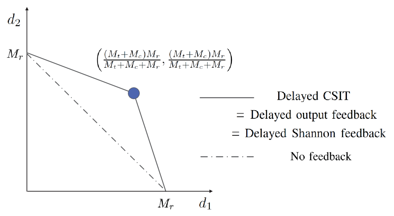
The outer bound of DoF region given in (2) will be derived in Theorem 6 of Section VI. We propose a coding scheme that achieves a $(d_{a},d_{b})=(\frac{2}{3},\frac{2}{3})$ DoF pair almost surely. The coding scheme is a modified version of the retrospective interference alignment in [15] for our channel model. The DoF tuple achieved by this scheme is a point on the DoF region as shown in Fig. 2. Then, we can also achieve the entire DoF region using time sharing.

Now, we show that the $(\frac{2}{3},\frac{2}{3})$ DoF pair is achievable under delayed CSIT. Time slots are partitioned into groups of three, and each transmitter sends two symbols during the 3 time slots, thus DoF of 2/3 is achieved per user. The transmit symbols of Transmitter $a$ are denoted as $S_{1a}$ and $S_{2a}$, and the transmit symbols for Transmitter $b$ are $Q_{1b}$ and $Q_{2b}$. The transmission mechanism is as follows: in the first time slot Transmitter $a$ and the cognitive relay transmit (different) random linear combinations of $S_{1a},S_{2a}$, while Transmitter $b$ is silent. Neglecting the noise terms, the received signals are:

All precoding variables are chosen so that power constraints are satisfied, but so that $\frac{u_{1a,1}}{u_{2a,1}}\neq\frac{v_{1c,1}}{v_{2c,1}}$. In time slot 2, a similar action takes place, except Transmitter $b$ and the cognitive relay transmit and Transmitter $a$ is silent.

where similar conditions on the precoding variables are imposed. Finally, in time slot 3, Transmitter $a$ and Transmitter $b$ transmit but the relay is silent. Using delayed CSIT, the transmitters respectively transmit the received signal at their non-intended receiver during the initial transmission, appropriately scaled to account for power constraints.

Subtracting $H_{ab,3}(p_{2}Y_{a,2})$ from $Y_{a,3}$ with the received signal at time index $t=2$, Receiver $a$ can obtain the interference-free signal $Y_{b,1}$ as

The signaling scheme is depicted in Fig. 3. We can readily know that $Y_{a,1}$ and $Y_{b,1}$ are almost surely linearly independent since channel gains are independently drawn from the same continuous distribution and $u_{ja,1}$ and $v_{ja,1},j\in\{1,2\}$, are also random and independent. Thus, Receiver $a$ has two independent equations given by linear combinations of two variables $S_{1a}$ and $S_{2a}$ so that it can decode two symbols. Similarly, since Receiver $b$ can obtain $Y_{a,2}$, Receiver $b$ also has two independent equations $Y_{a,2}$ and $Y_{b,2}$ of two variables intended for Receiver $b$, and hence Receiver $b$ can decode two symbols $Q_{1b}$ and $Q_{2b}$. Consequently, at the end of transmission, each receiver can achieve $\frac{2}{3}$ DoF (i.e., two symbols over 3 time slots) almost surely. In other words, the sum DoF is $\frac{4}{3}$. ∎

The outer bound is determined by $d_{a}+\frac{d_{b}}{2}\leq 1,\ \frac{d_{a}}{2}+d_{b}\leq 1$ that will be derived in Theorem  6 of Section VI. We propose a scheme that achieves $(d_{a},d_{b})=(\frac{2}{3},\frac{2}{3})$ DoF pair almost surely, a point that is on the outer bound, and then all other points on the outer bound are achieved via time sharing.

Similar to the delayed CSIT case, the achievable scheme needs $3$ time slots. At time slot 1 and 2, the signaling follows Section III-A. In time slot 3, however, a different signaling is used where the transmitter utilizes the output feedback from the receiver instead of constructing a linear combination of previous symbols based on delayed CSI. Each transmitter transmits the output fed back from the intended receiver, appropriately scaled to satisfy the power constraints.

Subtracting $H_{aa,3}(p_{1}Y_{a,2})$ from $Y_{a,3}$ with the received signal at time index $t=2$, Receiver $a$ can obtain the interference-free signal $Y_{b,1}$ as

The signaling scheme is shown in Fig. 4. Because Receiver $a$ almost surely has two linearly independent equations $Y_{a,1}$ and $Y_{b,1}$ that are linear combinations of two symbols $S_{1a}$ and $S_{2a}$, Receiver $a$ is able to decode the two symbols. Similarly, because Receiver $b$ can obtain $Y_{a,2}$ and almost surely has two linearly independent equations $Y_{a,2}$ and $Y_{b,2}$ of two symbols, Receiver $b$ can decode two symbols $Q_{1b}$ and $Q_{2b}$. As a result, each receiver can achieve $\frac{2}{3}$ DoF almost surely, and we can achieve $\frac{4}{3}$ sum DoF. ∎

The outer bound for delayed Shannon feedback is the same as that for delayed CSIT feedback or delayed output feedback. The outer bound is presented in Theorem 6 of Section VI. The outer bound can be achieved for the cases of delayed CSIT and delayed output feedback from Theorem 1 and Theorem 2. Therefore, the outer bound is also achievable because we can use both the delayed CSIT and the output feedback information. ∎

The DoF outer bound is $d_{a}+d_{b}\leq 1$ that will be proved in Corollary 5 of Section VI. The outer bound is achievable via time division multiplexing (TDM) when the transmitters and cognitive relay do not have any feedback information. ∎The result is true irrespective of the number of transmit or receive antennas. In section IV-D, we will show that TDM is also DoF optimal for the MIMO case.

We show the achievable DoF region according to the classified conditions, and compare the achievable DoF region with the DoF outer bound that will be derived in Theorem 6 of Section VI. The delayed CSIT is not used in the achievable scheme for Condition I, but we exploit delayed CSIT for Condition II, III, IV and V.

1. 1.

   Condition I: $M_{t}+M_{c}\leq M_{r}$

   In this case, the DoF outer bound with delayed CSIT is constructed from $d_{a}\leq M_{t}+M_{c},\ d_{b}\leq M_{t}+M_{c},$ and $d_{a}+d_{b}\leq\min(M_{r},2M_{t}+M_{c})$. Using a similar approach of decomposing an interference channel into multiple access channel (MAC) [28], we decompose the ICCR into MACs. The two users and the cognitive relay each use their own codewords. Since each receiver can decode the maximum of $\min(M_{r},2M_{t}+M_{c})$ signals, the two transmitters and cognitive relay send total $\min(M_{r},2M_{t}+M_{c})$ messages, then each receiver can decode all signals. Consequently, the optimal DoF region is obtained and the total sum DoF becomes $\min(M_{r},2M_{t}+M_{c})$.

2. 2.

   Condition II: $\frac{M_{t}+M_{c}}{2}\leq M_{r}<M_{t}+M_{c}$ and $M_{r}>M_{t}$

   A DoF outer bound with delayed CSIT for this case is given by $\frac{d_{a}}{M_{t}+M_{c}}+\frac{d_{b}}{M_{r}}\leq 1$ and $\frac{d_{a}}{M_{r}}+\frac{d_{b}}{M_{t}+M_{c}}\leq 1$. We can show that the DoF pair $\Big(\frac{(M_{t}+M_{c})M_{r}}{M_{r}+M_{t}+M_{c}},\frac{(M_{t}+M_{c})M_{r}}{{M_{r}}+M_{t}+M_{c}}\Big)$ is achievable, which lies on the intersection of $\frac{d_{a}}{M_{t}+M_{c}}+\frac{d_{b}}{M_{r}}\leq 1$ and $\frac{d_{a}}{M_{r}}+\frac{d_{b}}{M_{t}+M_{c}}\leq 1$ on the DoF outer bound. First, for each time slot $t\in\{1,\cdots,M_{r}\}$, Transmitter $a$ sends random linear combinations of $M_{t}+M_{c}$ independent symbols, and the cognitive relay sends different random linear combinations of the $M_{t}+M_{c}$ independent symbols. The received signals at time index $t\in\{1,\cdots,M_{r}\}$ can be represented as

   	$$Y_{a,t}=\mathbf{H}_{aa,t}\mathbf{U}_{a,t}S_{a,t}+\mathbf{H}_{1c,t}\mathbf{V}_{c,t}S_{a,t},$$		(11a)
   	$$Y_{b,t}=\mathbf{H}_{ba,t}\mathbf{U}_{a,t}S_{a,t}+\mathbf{H}_{2c,t}\mathbf{V}_{c,t}S_{a,t},$$		(11b)

   where $\mathbf{U}_{a,t}$ is a randomly chosen $M_{t}\times(M_{t}+M_{c})$ matrix with rank $M_{t}$, $\mathbf{V}_{c,t}$ is a randomly chosen $M_{c}\times(M_{t}+M_{c})$ matrix with rank $M_{c}$, $S_{a,t}$ is an $(M_{t}+M_{c})\times 1$ symbol vector for Receiver $a$ at time index $t$, the transmissions are appropriately scaled to satisfy the power constraint, and noise terms are omitted since noise does not affect DoF. Because Receiver $a$ obtains $M_{r}$ linear combinations of the desired $M_{t}+M_{c}$ variables at each time index, Receiver $a$ has total $M_{r}^{2}$ independent linear equations of the $(M_{t}+M_{c})M_{r}$ desired symbols during $M_{r}$ time slots.

   Then in each time slot $t\in\{M_{r}+1,\cdots,2M_{r}\}$, Transmitter $b$ and the cognitive relay send different random linear combinations of $M_{t}+M_{c}$ symbols intended for Receiver $b$. The received signals at time index $t\in\{M_{r}+1,\cdots,2M_{r}\}$ are

   	$$Y_{a,t}=\mathbf{H}_{ab,t}\mathbf{U}_{b,t}Q_{b,t}+\mathbf{H}_{1c,t}\mathbf{V}_{c,t}Q_{b,t},$$		(12a)
   	$$Y_{b,t}=\mathbf{H}_{bb,t}\mathbf{U}_{b,t}Q_{b,t}+\mathbf{H}_{2c,t}\mathbf{V}_{c,t}Q_{b,t},$$		(12b)

   where $\mathbf{U}_{b,t}$ is a randomly chosen $M_{t}\times(M_{t}+M_{c})$ matrix with rank $M_{t}$, $\mathbf{V}_{c,t}$ is a randomly chosen $M_{c}\times(M_{t}+M_{c})$ matrix with rank $M_{c}$, $Q_{b,t}$ is an $(M_{t}+M_{c})\times 1$ symbol vector for Receiver $b$ at time index $t$, all coefficients are appropriately selected to satisfy the power constraint, and noise terms are omitted. Receiver $b$ obtains total $M_{r}^{2}$ independent linear combinations of the $(M_{t}+M_{c})M_{r}$ desired variables during $M_{r}$ time slots.

   At time index $t\in\{2M_{r}+1,...,M_{t}+M_{c}+M_{r}\}$, Transmitter $a$, Transmitter $b$, and the cognitive relay transmit $X_{a,t}=[Y_{b[t-2M_{r}],1},...,Y_{b[t-2M_{r}],M_{t}}]^{T}$, $X_{b,t}=[Y_{a[t-2M_{r}],M_{r}+1},...,Y_{a[t-2M_{r}],M_{r}+M_{t}}]^{T}$ and $X_{c,t}=[Y_{b[t-2M_{r}],M_{t}+1}+Y_{a[t-2M_{r}],M_{r}+M_{t}+1},...,Y_{b[t-2M_{r}],M_{r}}+Y_{a[t-2M_{r}],2M_{r}},0,...,0]^{T}$, respectively, using delayed CSI. Note that the cognitive relay transmits $X_{c,t}$ using only $M_{r}-M_{t}$ antennas. The transmissions are appropriately scaled to satisfy the power constraint. The received signals at $t\in\{2M_{r}+1,\cdots,M_{t}+M_{c}+M_{r}\}$ are

   	$$Y_{a,t}=\mathbf{H}_{aa,t}X_{a,t}+\mathbf{H}_{ab,t}X_{b,t}+\mathbf{H}_{ac,t}X_{c,t},$$		(13a)
   	$$Y_{b,t}=\mathbf{H}_{ba,t}X_{a,t}+\mathbf{H}_{bb,t}X_{b,t}+\mathbf{H}_{bc,t}X_{c,t},$$		(13b)

   where noise terms are omitted. Since the interfering terms are comprised of the past received signal in previous slots, each receiver can eliminate the interfering terms using the received signals in the previous time slots and obtain $(M_{t}+M_{c}-M_{r})M_{r}$ linearly independent interference-free signals during $M_{t}+M_{c}-M_{r}$ time slots. Therefore, each receiver has $(M_{t}+M_{c})M_{r}$ linearly independent equations involving $(M_{t}+M_{c})M_{r}$ symbols and thus we can obtain the DoF pair $\Big(\frac{(M_{t}+M_{c})M_{r}}{M_{t}+M_{c}+M_{r}},\frac{(M_{t}+M_{c})M_{r}}{M_{t}+M_{c}+M_{r}}\Big)$ which is the same achievable DoF pair in Condition II. The other points on the DoF outer bound can be also achieved via time sharing.

3. 3.

   Condition III: $\frac{M_{t}+M_{c}}{2}\leq M_{r}<M_{t}+M_{c}$ and $M_{r}\leq M_{t}$

   We show that the $\Big(\frac{(M_{t}+M_{c})M_{r}}{M_{t}+M_{c}+M_{r}},\frac{(M_{t}+M_{c})M_{r}}{M_{t}+M_{c}+M_{r}}\Big)$ DoF pair is achievable, which is an intersection point of $\frac{d_{a}}{M_{t}+M_{c}}+\frac{d_{b}}{M_{r}}\leq 1$ and $\frac{d_{a}}{M_{r}}+\frac{d_{b}}{M_{t}+M_{c}}\leq 1$ on the DoF outer bound.

   First, we spend $2M_{r}$ time slots. At each time index $t\in\{1,\cdots,M_{r}\}$, Transmitter $a$ sends random linear combinations of $M_{t}+M_{c}$ independent symbols, and the cognitive relay sends different random linear combinations of the $M_{t}+M_{c}$ independent symbols. Since Receiver $a$ obtains $M_{r}$ linear combinations of the desired $M_{t}+M_{c}$ variables at each time index, Receiver $a$ has total $M_{r}^{2}$ independent linear equations of the $(M_{t}+M_{c})M_{r}$ desired symbols during $M_{r}$ time slots. At each time index $t\in\{N+1,\cdots,2M_{r}\}$, Transmitter $b$ and the cognitive relay send different random linear combinations of $M_{t}+M_{c}$ symbols intended for Receiver $b$. Receiver $b$ obtains total $M_{r}^{2}$ independent linear combinations of the $(M_{t}+M_{c})M_{r}$ desired variables during $M_{r}$ time slots.

   Second, we need $M_{t}+M_{c}-M_{r}$ time slots. At time index $t\in\{2M_{r}+1,\cdots,M_{t}+M_{c}+M_{r}\}$, Transmitter $a$ and Transmitter $b$ transmit $X_{a,t}=[Y_{b[t-2M_{r}],1},\cdots,Y_{b[t-2M_{r}],M_{r}},0,\cdots,0]^{T}$ and $X_{b,t}=[Y_{a[t-2M_{r}],M_{r}+1},\cdots,Y_{a[t-2M_{r}],2M_{r}},$ $0,\cdots,0]^{T}$, respectively, using only $M_{r}$ antennas. The cognitive relay does not transmit. Since Receiver $a$ knows $Y_{a[t-2M_{r}],M_{r}+1},$ $\cdots,Y_{a[t-2M_{r}],2M_{r}}$ and Receiver $b$ knows $Y_{b[t-2M_{r}],1},\cdots,Y_{b[t-2M_{r}],M_{r}}$ where $t\in\{2M_{r}+1,\cdots,M_{t}+M_{c}+M_{r}\}$, each receiver can eliminate interference terms and obtain $(M_{t}+M_{c}-M_{r})M_{r}$ linearly independent interference-free signals during $M_{t}+M_{c}-M_{r}$ time slots. Therefore, the receivers have total $(M_{t}+M_{c})M_{r}$ linearly independent equations involving $(M_{t}+M_{c})M_{r}$ symbols, respectively. Consequently, we can obtain the $\Big(\frac{(M_{t}+M_{c})M_{r}}{M_{t}+M_{c}+M_{r}},\frac{(M_{t}+M_{c})M_{r}}{M_{t}+M_{c}+M_{r}}\Big)$ DoF pair. The other points on the outer bound are achievable via time sharing.

4. 4.

   Condition IV: $M_{r}<\frac{M_{t}+M_{c}}{2}$ and $M_{r}>M_{t}$

   The DoF outer bound is determined by $\frac{d_{a}}{2M_{r}}+\frac{d_{b}}{M_{r}}\leq 1$ and $\frac{d_{a}}{M_{r}}+\frac{d_{b}}{2M_{r}}\leq 1$. We show that the $(\frac{2M_{r}}{3},\frac{2M_{r}}{3})$ DoF pair on the DoF outer bound is achievable. All transmissions are scaled to satisfy the power constraint. First, we spend two time slots. At time index $t=1$, Transmitter $a$ sends $M_{t}$ random linear combinations of $2M_{r}$ symbols, and the cognitive relay sends $2M_{r}-M_{t}$ different random linear combinations of the $2M_{r}$ symbols. The received signals at time index $t=1$ can be represented as

   	$$Y_{a,1}=\mathbf{H}_{aa,1}\mathbf{U}_{a,1}S_{a}+\mathbf{H}_{ac,1}\mathbf{V}_{c,1}S_{a}$$		(14a)
   	$$Y_{b,1}=\mathbf{H}_{ba,1}\mathbf{U}_{a,1}S_{a}+\mathbf{H}_{bc,1}\mathbf{V}_{c,1}S_{a},$$		(14b)

   where $\mathbf{U}_{a,1}$ is a randomly chosen $M_{t}\times(2M_{r})$ matrix with full rank, $\mathbf{V}_{c,1}$ is a randomly chosen $M_{c}\times(2M_{r})$ matrix with rank $M_{r}$ which includes a $(M_{c}-M_{r})\times(2M_{r})$ zero matrix, $S_{a}$ is a $(2M_{r})\times 1$ symbol vector for Receiver $a$, and noise terms are omitted. Receiver $a$ has $M_{r}$ linear combinations of intended $2M_{r}$ variables. Similarly, at time index $t=2$, Transmitter $b$ sends $M_{t}$ random linear combinations of $2M_{r}$ symbols intended for Receiver $b$, and the cognitive relay sends different $2M_{r}-M_{t}$ random linear combinations of the $2M_{r}$ symbols. The received signals at time index $t=2$ are

   	$$Y_{a,2}=\mathbf{H}_{ab,2}\mathbf{U}_{b,2}Q_{b}+\mathbf{H}_{ac,2}\mathbf{V}_{c,2}Q_{b},$$		(15a)
   	$$Y_{b,2}=\mathbf{H}_{bb,2}\mathbf{U}_{b,2}Q_{b}+\mathbf{H}_{bc,2}\mathbf{V}_{c,2}Q_{b},$$		(15b)

   where $\mathbf{U}_{b,2}$ is a randomly chosen $M_{t}\times(2M_{r})$ matrix with full rank, $\mathbf{V}_{c,2}$ is a randomly chosen $M_{c}\times(2M_{r})$ matrix with rank $M_{r}$ which includes a $(M_{c}-M_{r})\times(2M_{r})$ zero matrix, and $Q_{b}$ is a $(2M_{r})\times 1$ symbol vector for Receiver $b$. Receiver $b$ obtains $M_{r}$ linear combinations of intended $2M_{r}$ variables.

   Second, we need one time slot indexed by $t=3$. Transmitter $a$, Transmitter $b$, and the cognitive relay transmit $X_{a,3}=[Y_{b[1],1},...,Y_{b[M_{t}],1}]^{T}$, $X_{b,3}=[Y_{a[1],2},...,Y_{a[M_{t}],2}]^{T}$ and $X_{c,3}=[Y_{b[M_{t}+1],1}+Y_{a[M_{t}+1],2},...,Y_{b[M_{r}],1}+Y_{a[M_{r}],2},0,...,0]^{T}$, respectively, using delayed CSI. At time index $t=3$, the received signals are

   	$$Y_{a,3}=\mathbf{H}_{aa,3}X_{a,3}+\mathbf{H}_{ab,3}X_{b,3}+\mathbf{H}_{ac,3}X_{c,3},$$		(16a)
   	$$Y_{b,3}=\mathbf{H}_{ba,3}X_{a,3}+\mathbf{H}_{bb,3}X_{b,3}+\mathbf{H}_{bc,3}X_{c,3}.$$		(16b)

   Since the interference terms at each receiver are comprised of the received signals in the previous time slots, each receiver can obtain $M_{r}$ linearly independent interference-free signals at $t=3$. Thus, each receiver has total $2M_{r}$ linearly independent equations involving $2M_{r}$ symbols and thus we can obtain the $(\frac{2M_{r}}{3},\frac{2M_{r}}{3})$ DoF pair which is the same achievable DoF pair in Condition V. We can achieve all points on the DoF outer bound via time sharing.

5. 5.

   Condition V: $M_{r}<\frac{M_{t}+M_{c}}{2}$ and $M_{r}\leq M_{t}$

   In this case a DoF outer bound is given by $\frac{d_{a}}{2M_{r}}+\frac{d_{b}}{M_{r}}\leq 1$ and $\frac{d_{a}}{M_{r}}+\frac{d_{b}}{2M_{r}}\leq 1$. We show that the $(\frac{2M_{r}}{3},\frac{2M_{r}}{3})$ DoF pair on the DoF outer bound is achievable.

   At time index $t=1$, if $2M_{r}>M_{t}$, Transmitter $a$ sends $M_{t}$ random linear combinations of $2M_{r}$ symbols with $M_{t}$ transmit antennas, and the cognitive relay sends $2M_{r}-M_{t}$ different random linear combinations of the $2M_{r}$ symbols. If $2M_{r}\leq M_{t}$, then Transmitter $a$ only transmits and the cognitive relay is silent. The received signals at time index $t=1$ can be represented as (14a) and (14b) where $\mathbf{U}_{a,1}$ is a randomly chosen $M_{t}\times 2M_{r}$ matrix with full rank, $\mathbf{V}_{c,1}$ is a randomly chosen $M_{c}\times 2M_{r}$ matrix with rank $(2M_{r}-M_{t})^{+}$ which includes a $(M_{c}-(2M_{r}-M_{t})^{+})\times 2M_{r}$ zero matrix, $(x)^{+}=\max(x,0)$, $S_{a}$ is a $2M_{r}\times 1$ symbol vector for Receiver $a$, and noise terms are omitted. Receiver $a$ has $M_{r}$ linear combinations of intended $2M_{r}$ variables. Similarly, at time index $t=2$, Transmitter $b$ sends $M_{t}$ random linear combinations of $2M_{r}$ symbols intended for Receiver $b$, and the cognitive relay sends different $2M_{r}-M_{t}$ random linear combinations of the $2M_{r}$ symbols if $2M_{r}>M_{t}$. If $2M_{r}\leq M_{t}$, then Transmitter $b$ only transmits and the cognitive relay becomes silent. The received signals at time index $t=2$ are the same as (15a) and (15b) where $\mathbf{U}_{b,2}$ is a randomly chosen $M_{t}\times 2M_{r}$ matrix with full rank, $\mathbf{V}_{c,2}$ is a randomly chosen $M_{c}\times 2M_{r}$ random matrix with rank $(2M_{r}-M_{t})^{+}$ which includes a $(M_{c}-(2M_{r}-M)^{+})\times 2M_{r}$ zero matrix, and $Q_{b}$ is a $2M_{r}\times 1$ symbol vector for Receiver $b$. Receiver $b$ obtains $M_{r}$ linear combinations of the intended $2M_{r}$ variables.

   At time index $t=3$, Transmitter $a$ and Transmitter $b$ only transmit $X_{a,3}=[Y_{b[1],1},\cdots,Y_{b[M_{r}],1},0,$ $\cdots,0]^{T}$ and $X_{b,3}=[Y_{a[1],2},\cdots,Y_{a[M_{r}],2},0,\cdots,0]^{T}$, respectively, using $M_{r}$ antennas, and the cognitive relay does not transmit. Since the interference signals at each receiver at $t=3$ are the received signals in previous time slots, each receiver can obtain $M_{r}$ linearly independent interference-free signals at $t=3$. Thus, each receiver has total $2M_{r}$ linearly independent equations involving $2M_{r}$ symbols and hence we can obtain the $(\frac{2M_{r}}{3},\frac{2M_{r}}{3})$ DoF pair on the DoF outer bound. The other points on the outer bound are achievable via time sharing.

References

- [1] M. Kang and W. Choi, “ The capacity of a three-user interference channel with a cognitive transmitter in strong interference,” in Proc. IEEE Int. Symp. Info. Theory, Cambridge, MA, Jul. 2012.
- [2] O. Sahin and E. Erkip, “On achievable rates for interference relay channel with interference cancellation,” in Proc. Asilomar Conf. Signals, Systems and Computers, Pacific Grove, CA, Nov. 2007.
- [3] M. Costa, “Writing on dirty paper (corresp.),” IEEE Trans. Info. Theory, vol. 29, no. 3, pp. 439-441, May 1983.
- [4] S. Sridharan, S. Vishwanath, S. A. Jafar, and S. Shamai, “On the capacity of cognitive relay assisted Gaussian interference channel,” in Proc. IEEE Int. Symp. Info. Theory, Toronto, Ontario, Canada, Jul. 2008.
- [5] T. S. Han and K. Kobayashi, “A new achievable rate region for the interference channel,” IEEE Trans. Info. Theory, vol. 27, no. 1, pp. 49–60, Jan. 1981.
- [6] S. Rini, D. Tuninetti, and N. Devroye, “Outer bounds for the interference channel with a cognitive relay,” in Proc. IEEE Information Theory Workshop, Dublin, Ireland, Sep. 2010.
- [7] S. Rini, D. Tuninetti, N. Devroye, and A. Goldsmith, “The capacity of the interference channel with a cognitive relay in strong interference.” in Proc. IEEE Int. Symp. Info. Theory, St. Petersburg, Russia, Jul. 2011.
- [8] ——, “On the capacity of the interference channel with a cognitive relay,” IEEE Trans. Info. Theory, vol. 60, no. 4, pp. 2148-2179, Apr. 2014.
- [9] H. Charmchi, G. A. Hodtani, and M. Nasiri-Kenari, “A new outer bound for a class of interference channels with a cognitive relay and a certain capacity result,” IEEE Communications Letters, vol. 17, no. 2, pp. 241-244, Feb. 2013.
- [10] A. Dytso, S. Rini, N. Devroye, and D. Tuninetti, “On the capacity region of the two-user interference channel with a cognitive relay,” IEEE Trans. Wireless Commun., vol. 13, no. 12, pp. 6824-6838, Dec. 2014.
- [11] A. Chaaban and A. Sezgin, “The DoF of the K-user interference channel with a cognitive relay,” in Proc. IEEE Int. Symp. Info. Theory, Cambridge, MA, Jul. 2012.
- [12] C. Wang and A. Sezgin, “Degrees of freedom of the interference channel with a cognitive helper,” IEEE Communications Letters, vol. 17, no. 5, pp. 920-923, May 2013.
- [13] R. A. Tannious and A. Nosratinia, “Relay-assisted interference network: degrees of freedom,” IEEE Trans. Info. Theory, vol. 58, no. 6, pp. 3780-3786, Jun. 2012.
- [14] V. R. Cadambe and S. A. Jafar, “Interference alignment and degrees of freedom of the K-user interference channel,” IEEE Trans. Info. Theory, vol. 54, no. 8, pp. 3425-3441, Aug. 2008.
- [15] M. A. Maddah-Ali and D. Tse, “Completely stale transmitter channel state information is still very useful,” IEEE Trans. Info. Theory, vol. 58, no. 7, pp. 4418-4431, Jul. 2012.
- [16] C. S. Vaze and M. K. Varanasi, “The degrees of freedom region of the two-user MIMO broadcast channel with delayed CSIT,” in Proc. IEEE Int. Symp. Info. Theory, St. Petersburg, Russia, Jul. 2011.
- [17] M. J. Abdoli, A. Ghasemi, and A. K. Khandani, “On the degrees of freedom of three-user MIMO broadcast channel with delayed CSIT,” in Proc. IEEE Int. Symp. Info. Theory, St. Petersburg, Russia, Jul. 2011.
- [18] H. Maleki, S. A. Jafar, and S. Shamai, “Retrospective interference alignment over interference networks,” IEEE J. Sel. Topics in Sig. Processing, vol. 6, no. 3, pp. 228-240, Jun. 2012.
- [19] M. J. Abdoli, A. Ghasemi, and A. K. Khandani, “On the degrees of freedom of -user SISO interference and X channels with delayed CSIT.” Available: http://arxiv.org/abs/1109.4314, 2011.
- [20] A. Ghasemi, A. S. Motahari, and A. K. Khandani, “ On the degrees of freedom of X channel with delayed CSIT,” in Proc. IEEE Int. Symp. Info. Theory, St. Petersburg, Russia, Jul. 2011.
- [21] M. G. Kang and W. Choi , “Ergodic interference aligment with delayed feedback.” IEEE Sig. Processing Letters, vol. 20, no. 5, pp. 511-514, May 2013.
- [22] C. S. Vaze and M. K. Varanasi, “The degrees of freedom region and interference alignment for the MIMO interference channel with delayed CSIT,” IEEE Trans. Info. Theory, vol. 58, no. 7, pp. 4396-4417, Jul. 2012.
- [23] R. Tandon, S. Mohajer, H. V. Poor, and S.Shamai, “Degrees of freedom region of the MIMO interference channel with output feedback and delayed CSIT,” IEEE Trans. Info. Theory, vol. 59, no. 3, pp. 1444-1457, Mar. 2013.
- [24] A. Ghasemi, A. S. Motahari, and A. K. Khandani, “Interference alignment for the MIMO interference channel with delayed local CSIT.” Available: http://arxiv.org/abs/1102.5673, 2011.
- [25] K. Mohanty, C. S. Vaze, and M. K. Varanasi, “The degrees of freedom region for the MIMO interference channel with hybrid CSIT,” IEEE Trans. Info. Theory, to be publised.
- [26] C. Huang, S. A. Jafar, S. Shamai, and S. Vishwanath, “On degrees of freedom region of MIMO networks without channel state information at transmitters,” IEEE Trans. Info. Theory, vol. 58, no. 2, pp. 849-857, Feb. 2012.
- [27] C. S. Vaze and M. K. Varanasi, “The degree-of-freedom regions of MIMO broadcast, interference, and cognitive radio channels with no CSIT,” IEEE Trans. Info. Theory, vol. 58, no. 8, pp. 5354-5374, Aug. 2012.
- [28] A. B. Carleial, “Interference channels,” IEEE Trans. Info. Theory, vol. 24, no. 1, pp. 60–70, Jan. 1978.
- [29] N. Devroye, P. Mitran and V. Tarokh, “Achievable rates in conitive radio channels,” IEEE Trans. Info. Theory, vol. 52, no. 5, pp. 1813-1827, May. 2006.
- [30] I. Maric, R. D. Yates and G. Kramer, “Capacity of interference channels with partial transmitter cooperation,” IEEE Trans. Info. Theory, vol. 53, no. 10, pp. 3536-3548 , Oct. 2007.
- [31] I. Maric, A. Goldsmith, G. Kramer and S. Shamai, “On the capacity of interference channels with one cooperating transmitter,” Eur. Trans. Telecomms, vol. 19, no. 4, pp. 405-420 , Jun. 2008.
- [32] S. Rini and A. Goldsmith, “On the capacity of the MIMO cognitive interference channel,” in Proc. IEEE Int. Symp. Info. Theory, Istanbul, Turkey, Jul. 2013.
- [33] ——, “On the capacity of the multiantenna Gaussian cognitive interference channel,” IEEE J. Sel. Areas Commun., vol. 32, no. 11, pp. 2252-2267 , Nov. 2014.
- [34] C. Huang and S. A. Jafar, “Degrees of freedom of the MIMO interference channel with cooperation and cognition,” IEEE Trans. Info. Theory, vol. 55, no. 9, pp. 4211–4220, Sep. 2009.