Centrosymmetric Matrices in the Sinc Collocation Method for Sturm-Liouville Problems

In science and engineering, differential eigenvalue problems occur abundantly. Differential eigenvalue problems can arise when partial differential equations are solved using the method of separation of variables. Consequently, they also play an important role in Sturm-Liouville (SL) differential eigenvalue problems [1]. For example, the solution of the wave equation can be expressed as the sum of standing waves. The frequencies of these standing waves are precisely the eigenvalues of its corresponding Sturm-Liouville problem. Similarly, in quantum mechanics, the energy eigenvalues associated with a Hamiltonian operator are modelled using the time-independent Schrödinger equation which is in fact a special case of a Sturm-Liouville differential eigenvalue problem.

Recently, collocation and spectral methods have shown great promise for solving singular Sturm-Liouville differential eigenvalue problems [2, 3]. More specifically, the Sinc collocation method (SCM) [4, 5, 6] has been shown to yield exponential convergence. During the last three decades the SCM has been used extensively to solve many problems in numerical analysis. The applications include numerical integration, linear and non-linear ordinary differential equations, partial differential equations, interpolation and approximations to functions [7, 8]. The SCM applied to Sturm-Liouville problems consists of expanding the solution of a SL problem using a basis of Sinc functions. By evaluating the resulting approximation at the Sinc collocation points separated by a fixed mesh size $h$, one obtains a matrix eigenvalue problem or generalized matrix eigenvalue problem for which the eigenvalues are approximations to the eigenvalues of the SL operator. In [9], we used the double exponential Sinc collocation method (DESCM) to compute the eigenvalues of singular Sturm-Liouville boundary value problems. The DESCM leads to a generalized eigenvalue problem where the matrices are symmetric and positive-definite. In addition, we demonstrate that the convergence of the DESCM is of the rate ${\cal O}\left(\frac{N^{5/2}}{\log(N)^{2}}e^{-\kappa N/\log(N)}\right)$ for some $\kappa>0$ as $N\to\infty$, where $2N+1$ is the dimension of the resulting generalized eigenvalue system. The DESCM was also applied successfully to the Schrödinger equation with the anharmonic oscillators [10].

In the present contribution, we show how a parity symmetry of the Sturm-Liouville operator can be conserved and exploited when converting our differential eigenvalue problem into a matrix eigenvalue problem. Indeed, given certain parity assumptions, the matrices resulting from the DESINC method are not only symmetric and positive definite; they are also centrosymmetric. The study of centrosymmetry has a long history [11, 12, 13, 14, 15, 16, 17, 18]. However, the last two decades has stemmed much research focused on the properties and applications of centrosymmetric matrices ranging from iterative methods for solving linear equations to least-squares problems to inverse eigenvalue problems [19, 20, 21, 22, 23, 24, 25, 26, 27, 28, 29, 30, 31, 32, 33].

Using the eigenspectrum properties of symmetric centrosymmetric matrices presented in [12], we apply the DESCM algorithm to Sturm-Liouville eigenvalue problems and demonstrate that solving the resulting generalized eigensystem of dimension $(2N+1)\times(2N+1)$ is equivalent to solving the two smaller eigensystems of dimension $N\times N$ and $(N+1)\times(N+1)$. Moreover, we also demonstrate that only $\frac{1}{N+1}$ of all components need to be stored at every iteration in order to obtain all generalized eigenvalues. To illustrate the gain in efficiency obtained by this method, we apply the DESCM method to the time independent Schrödinger equation with an anharmonic potential. Furthermore, it is worth mentioning that research concerning inverse eigenvalue problems where the matrices are assumed centrosymmetric has been the subject of much research recently [28, 23]. Consequently, the combination of these results and our findings could lead to a general approach for solving inverse Sturm-Liouville problems.

All calculations are performed using the programming language Julia and all the codes are available upon request.

The sinc function valid for all $z\in\mathbb{C}$ is defined by the following expression:

$$\textrm{sinc}(z)=\left\{\begin{array}[]{cc}\dfrac{\sin(\pi z)}{\pi z}&\quad\textrm{for}\quad z\neq 0\\[8.5359pt] 1&\quad\textrm{for}\quad z=0.\end{array}\right.$$

(1)

For $j\in\mathbb{Z}$ and $h$ a positive number, we define the Sinc function $S(j,h)(x)$ by:

$$S(j,h)(x)=\textrm{sinc}\left(\dfrac{x-jh}{h}\right)\quad\textrm{for}\quad x\in\mathbb{C}.$$

(2)

The Sinc function defined in (2) form an interpolatory set of functions with the discrete orthogonality property:

$$S(j,h)(kh)=\delta_{j,k}\qquad\textrm{for}\qquad j,k\in\mathbb{Z},$$

(3)

where $\delta_{j,k}$ is the Kronecker delta function.

The Sturm-Liouville (SL) equation in Liouville form is defined as follows:

	$\displaystyle Lu(x)$	$\displaystyle=-u^{\prime\prime}(x)+q(x)u(x)\,=\,\lambda\rho(x)u(x)$
		$\displaystyle\hskip-14.22636pta<x<b\qquad\qquad u(a)=u(b)=0,$		(5)

where $-\infty\leq a<b\leq\infty$. Moreover, we assume that the function $q(x)$ is non-negative and the weight function $\rho(x)$ is positive. The values $\lambda$ are known as the eigenvalues of the SL equation.

In [34], we apply the DESCM to obtain an approximation to the eigenvalues $\lambda$ of equation (5). We initially applied Eggert et al.’s transformation to equation (5) since it was shown that the proposed change of variable results in a symmetric discretized system when using the Sinc collocation method [35]. The proposed change of variable is of the form [35, Defintion 2.1]:

$$v(x)=\left(\sqrt{(\phi^{-1})^{\prime}}\,u\right)\circ\phi(x)\qquad\Longrightarrow\qquad u(x)=\dfrac{v\circ\phi^{-1}(x)}{\sqrt{(\phi^{-1}(x))^{\prime}}},$$

(6)

where $\phi^{-1}(x)$ is a conformal map of a simply connected domain in the complex plane with boundary points $a\neq b$ such that $\phi^{-1}(a)=-\infty$ and $\phi^{-1}(b)=\infty$.

Applying the change of variable (6) into equation (5), one obtains [35]:

$$\mathcal{L}\,v(x)=-v^{\prime\prime}(x)+\tilde{q}(x)v(x)=\lambda\rho(\phi(x))(\phi^{\prime}(x))^{2}v(x)\quad\textrm{with}\quad\lim_{|x|\to\infty}v(x)=0,$$

(7)

where:

$$\tilde{q}(x)=-\sqrt{\phi^{\prime}(x)}\,\dfrac{{\rm d}}{{\rm d}x}\left(\dfrac{1}{\phi^{\prime}(x)}\dfrac{{\rm d}}{{\rm d}x}(\sqrt{\phi^{\prime}(x)})\right)+(\phi^{\prime}(x))^{2}q(\phi(x)).$$

(8)

To implement the double exponential transformation, we use a conformal mapping $\phi(x)$ such that the solution to equation (7) decays double exponentially. In other words, we need to find a function $\phi(x)$ such that:

$$|v(x)|\leq A\exp\left(-B\exp\left(\gamma|x|\right)\right),$$

(9)

for some positive constants $A,B,\gamma$. Examples of such mappings are given in [34, 36].

Applying the SCM method, we obtain the following generalized eigenvalue problem:

$\displaystyle\mathcal{L}\,{\bf C}_{M}(v,h)$

$\displaystyle={\bf A}{\bf v}\,=\,\mu{\bf D}^{2}{\bf v}\quad\Longrightarrow\quad({\bf A}-\mu{\bf D}^{2}){\bf v}\,=\,0,$

(10)

where the vectors ${\bf v}$ and ${\bf C}_{M}(v,h)$ are given by:

$${\bf v}=(v_{-N,h},\ldots,v_{N,h})^{T}\qquad\textrm{and}\qquad{\bf C}_{N}(v,h)=(C_{N}(v,h)(-Nh),\ldots,C_{N}(v,h)(Nh))^{T},$$

(11)

and $\mu$ are approximations of the eigenvalues $\lambda$ of equation (7). For more details on the application of the SCM, we refer the readers to [9].

As in [37], we let $\delta^{(l)}_{j,k}$ denote the $l^{\rm th}$ Sinc differentiation matrix with unit mesh size:

$$\delta^{(l)}_{j,k}=h^{l}\left.\left(\dfrac{\rm d}{{\rm d}x}\right)^{l}S(j,h)(x)\right|_{x=kh}.$$

(12)

The entries $A_{j,k}$ of the $(2N+1)\times(2N+1)$ matrix ${\bf A}$ are then given by:

$$A_{j,k}=-\dfrac{1}{h^{2}}\,\delta^{(2)}_{j,k}+\tilde{q}(kh)\,\delta^{(0)}_{j,k}\qquad{\rm with}\qquad-N\leq j,k\leq N,$$

(13)

and the entries $D^{2}_{j,k}$ of the $(2N+1)\times(2N+1)$ diagonal matrix ${\bf D}^{2}$ are given by:

$$D^{2}_{j,k}=(\phi^{\prime}(kh))^{2}\rho(\phi(kh))\,\delta^{(0)}_{j,k}\qquad{\rm with}\qquad-N\leq j,k\leq N.$$

(14)

As previously mentioned, Eggert et al.’s transformation leads to the matrices $\,{\bf A}$ and ${\bf D}^{2}$ to be symmetric and positive definite. However, as will be illustrated in the next section, given certain parity assumptions, these matrices yield even more symmetry.

In this section, we present some properties of the matrix $\,{\bf A}$ and ${\bf D}^{2}$ that will be beneficial in the computation of their eigenvalues. The matrices ${\bf A}$ and ${\bf D}^{2}$ are symmetric positive definite matrices when equation (7) is discretized using the Sinc collocation method. Additionally, given certain parity assumptions on the functions $q(x)$, $\phi(x)$ and $\rho(x)$ in equation (7), the matrices ${\bf A}$ and ${\bf D}^{2}$ will also be centrosymmetric.

We now present the following Theorem establishing the connection between symmetries of the Sturm-Liouville operator and its resulting matrix approximation.

Proof   The commutator $[\mathcal{L},\mathcal{J}]=0$ if and only if $q(x)$ and $\rho(x)$ are even functions and $\phi(x)$ is an odd function.

If $\phi(x)$ is an odd function, then $\phi^{\prime}(x)$ is even, $\phi^{\prime\prime}(x)$ is odd and $\phi^{\prime\prime\prime}(x)$ is even. From this and equation (8), it follows that $\tilde{q}(x)$ is even.

In order to show that the resulting matrices $\,{\bf A}$ and ${\bf D}^{2}$ are centrosymmetric, we demonstrate that both these matrices satisfy equation (20). Before doing so, it is important to notice that the $l^{\rm th}$ Sinc differentiation matrices defined in equation (12) have the following symmetric properties:

$\displaystyle\delta^{(l)}_{-j,-k}$

$\displaystyle=h^{l}\left.\left(\dfrac{\rm d}{{\rm d}x}\right)^{l}S(-j,h)(x)\right|_{x=-kh}\,=\,\begin{cases}\penalty\ \penalty\ \delta^{(l)}_{j,k}&\textrm{if}\quad\textrm{$l$ is even}\\[2.84544pt] -\delta^{(l)}_{j,k}&\textrm{if}\quad\textrm{$l$ is odd}.\end{cases}$

(22)

Hence, the $l^{\rm th}$ Sinc differentiation matrices are centrosymmetric if $l$ is even. It is worth noting that when $l$ is odd, the Sinc differentiation matrices are skew-centrosymmetric [27]. Consequently, investigating the form for the components of the matrix ${\bf A}$ in equation (13), we obtain:

	$\displaystyle A_{-j,-k}$	$\displaystyle=$	$\displaystyle-\dfrac{1}{h^{2}}\,\delta^{(2)}_{-j,-k}+\tilde{q}(-kh)\,\delta^{(0)}_{-j,-k}$		(23)
		$\displaystyle=$	$\displaystyle-\dfrac{1}{h^{2}}\,\delta^{(2)}_{j,k}+\tilde{q}(kh)\,\delta^{(0)}_{j,k}$
		$\displaystyle=$	$\displaystyle A_{j,k}.$

Similarly, investigating the form for the components of the matrix ${\bf D}^{2}$ in equation (14), we obtain:

	$\displaystyle D^{2}_{-j,-k}$	$\displaystyle=$	$\displaystyle(\phi^{\prime}(-kh))^{2}\rho(\phi(-kh))\,\delta^{(0)}_{-j,-k}$		(24)
		$\displaystyle=$	$\displaystyle(\phi^{\prime}(kh))^{2}\rho(\phi(kh))\,\delta^{(0)}_{j,k}$
		$\displaystyle=$	$\displaystyle D^{2}_{j,k}.$

Both matrices ${\bf A}$ and ${\bf D}^{2}$ satisfy equation (20). From this it follows that ${\bf A}$ and ${\bf D}^{2}$ are centrosymmetric.

Theorem 3.5 illustrates that Sinc basis functions preserve the parity property of the Sturm-Liouville operator when discretized. Hence, when the matrices $\,{\bf A}$ and ${\bf D}^{2}$ are symmetric centrosymmetric positive definite matrices, we can utilize these symmetries when solving for their generalized eigenvalues. In [12], Cantoni et al. proved several properties of symmetric centrosymmetric matrices. In the following, we will utilize some of these properties to facilitate our task of obtaining approximations to the generalized eigenvalues of the matrices $\,{\bf A}$ and ${\bf D}^{2}$. The following lemma will demonstrate the internal block structure of symmetric centrosymmetric matrices.

The next lemma simplifies the calculation needed to solve for these eigenvalues.

Cantoni et al. use Lemmas 3.6 and 3.7 to prove the following Theorem concerning a standard eigenvalue problem where the matrix is centrosymmetric.

Since our problem consists of solving a generalized eigenvalue problem where one matrix is a full symmetric centrosymmetric and the other is a diagonal centrosymmetric matrix, we propose the following Theorem.

Proof   This proof relies on the unitary transformation matrix presented in [12, Lemma 3]:

$${\bf K}=\dfrac{1}{\sqrt{2}}\left[\begin{array}[]{cccc}{\bf I}&{\bf 0}&-{\bf J}\\ {\bf 0}&\sqrt{2}&{\bf 0}\\ {\bf I}&{\bf 0}&{\bf J}\end{array}\right],$$

(30)

where ${\bf I}$ is the identity matrix and ${\bf J}$ is the exchange matrix.

It is easy to verify that:

$${\bf K}{\bf H}{\bf K^{T}}={\bf V},$$

(31)

where ${\bf V}$ is the matrix in lemma 3.7.

This result is analogous for the matrix ${\bf W}$ with a change in notation. Hence:

	$\displaystyle 0=$	$\displaystyle\det({\bf H}-\lambda{\bf W})$
	$\displaystyle=$	$\displaystyle\det({\bf K})\det({\bf H}-\lambda{\bf W})\det({\bf K^{T}})$
	$\displaystyle=$	$\displaystyle\det({\bf KHK^{T}}-\lambda{\bf KWK^{T}})$
	$\displaystyle=$	$\displaystyle\det\left(\left[\begin{array}[]{cccc}{\bf S-JC}&{\bf 0}&{\bf 0}\\ {\bf 0}&h&\sqrt{2}\penalty\ {\bf x^{T}}\\ {\bf 0}&\sqrt{2}\penalty\ {\bf x}&{\bf S+JC}\end{array}\right]-\lambda\left[\begin{array}[]{cccc}\mathrm{diag}\,({\bf w})&{\bf 0}&{\bf 0}\\ {\bf 0}&w&{\bf 0}\\ {\bf 0}&{\bf 0}&\mathrm{diag}\,({\bf w})\end{array}\right]\right)$
	$\displaystyle=$	$\displaystyle\det({\bf S-JC}-\lambda\mathrm{diag}\,({\bf w}))\det\left(\left[\begin{array}[]{cccc}h&\sqrt{2}\penalty\ {\bf x^{T}}\\ \sqrt{2}\penalty\ {\bf x}&{\bf S+JC}\end{array}\right]-\lambda\left[\begin{array}[]{cccc}w&{\bf 0}\\ {\bf 0}&\mathrm{diag}\,({\bf w})\end{array}\right]\right),$

from which the result follows.

Theorem 3.9 is very useful when $N$ is large since it is less costly to solve two symmetric generalized eigensystems of dimensions $N\times N$ and $(N+1)\times(N+1)$ rather than one symmetric eigensystem of dimension $(2N+1)\times(2N+1)$. Additionally, Lemma 3.6 also has large ramifications when it comes to saving storage space. As is discussed in [37], the $l^{\rm th}$ Sinc differentiation matrices are symmetric toeplitz matrices. Therefore, for a symmetric toeplitz matrix of dimension $(2N+1)\times(2N+1)$, only $2N+1$ elements need to be stored. Investigating the definition of the matrix ${\bf A}$ in equation (13), we can see that ${\bf A}$ is defined as the sum of a symmetric toeplitz matrix and a diagonal matrix. Moreover, from Lemma 3.6 and Theorem 3.9, using only the antidiagonal and anti-upper triangular half of matrix ${\bf C}$, the vector ${\bf x}$, the scalar $h$, the diagonal and lower triangular half of the matrix ${\bf S}$, the vector ${\bf w}$ and the scalar $w$, we can create all the elements needed to solve for the generalized eigenvalues of the matrices ${\bf A}$ and ${\bf D}^{2}$. Hence, the ratio of elements needed to be computed and stored at each iteration $N$ in order to solve for these eigenvalues is given by:

$$\textrm{Proportion of Entries Needed}\,=\,\dfrac{\left(2N+N+1\right)+\left(N+1\right)}{(2N+1)^{2}+(2N+1)}\,=\,\dfrac{1}{N+1}.$$

(41)

Thus, only $\frac{1}{N+1}$ of the entries need to be generated and stored at every iteration to obtain all of the generalized eigenvalues.

In the following section, we will illustrate the gain in efficiency of these results by applying the DESCM to the Schrödinger equation with an anharmonic oscillator.

The time independent Schrödinger equation given by:

$${\cal H}\,\psi(x)\,\,=\,E\,\psi(x)\qquad\textrm{with}\qquad\lim_{|x|\to\infty}\psi(x)=0.$$

(42)

In equation (42), the Hamiltonian is given by the following linear operator:

$${\cal H}=-\dfrac{{\rm d}^{2}}{{\rm d}x^{2}}+V(x),$$

where $V(x)$ is the potential energy function and $E$ is the energy eigenvalue of the hamiltonian operator ${\cal H}$. In our case, we are treating the anharmonic oscillator potential $V(x)$ defined by:

$$V(x)=\displaystyle\sum_{i=1}^{m}c_{i}x^{2i}\qquad\textrm{with}\qquad c_{m}>0\quad\textrm{and}\quad m\in\mathbb{N}\backslash\{1\}.$$

(43)

In [10], we successfully applied the DESCM to time independent Schrödinger equation with an anharmonic potential. As we can see, the time independent Schrödinger equation (42) is a special case of a Sturm-Liouville equation with $q(x)=V(x)$ and $\rho(x)=1$. Applying Eggert et al.’s transformation and the DESCM with $\phi(x)=\sinh(x)$, we arrived at the following generalized eigenvalue problem:

$$\det({\bf A}-\mathcal{E}{\bf D}^{2})=0,$$

(44)

where $\mathcal{E}$ are approximations of the energy eigenvalues $E$.

The matrices ${\bf A}$ and ${\bf D}^{2}$ defined by equation (13) and (14) are given by:

$$A_{j,k}=-\left(\dfrac{1}{h^{2}}\right)\delta^{(2)}_{j,k}\,+\tilde{V}(kh)\delta^{(0)}_{j,k}\quad{\rm with}\quad-N\leq j,k\leq N,$$

(45)

where:

$$\tilde{V}(x)\,=\,\dfrac{1}{4}-\dfrac{3}{4}\,\mathrm{sech}^{2}(x)+\cosh^{2}(x)\displaystyle\sum_{i=1}^{m}c_{i}\sinh^{2i}(x),$$

(46)

and:

$$D^{2}_{j,k}=\cosh^{2}(kh)\,\delta^{(0)}_{j,k}\qquad{\rm with}\qquad-N\leq j,k\leq N.$$

(47)

Since the anharmonic potential $V(x)$ defined in (43) is an even function, the function $\rho(x)=1$ is an even function and the conformal map $\phi(x)=\sinh(x)$ is an odd function, we know that Theorem 3.5 applies. Hence, the matrices ${\bf A}$ and ${\bf D}^{2}$ are symmetric centrosymmetric.

In this section, we test the computational efficiency of the results obtained in Theorem 3.9. All calculations are performed using the programming language Julia in double precision. The eigenvalue solvers in Julia use the linear algebra package LAPACK.

In [40], Chaudhuri et al. presented several potentials with known analytic solutions for energy levels calculated using supersymmetric quantum mechanics, namely:

$$\begin{array}[]{lllll}V_{1}(x)&=&x^{2}-4x^{4}+x^{6}&\Rightarrow&E_{0}=-2\\ V_{2}(x)&=&4x^{2}-6x^{4}+x^{6}&\Rightarrow&E_{1}=-9\\ V_{3}(x)&=&(105/64)x^{2}-(43/8)x^{4}+x^{6}-x^{8}+x^{10}&\Rightarrow&E_{0}=3/8\\ V_{4}(x)&=&(169/64)x^{2}-(59/8)x^{4}+x^{6}-x^{8}+x^{10}&\Rightarrow&E_{1}=9/8.\end{array}$$

(48)

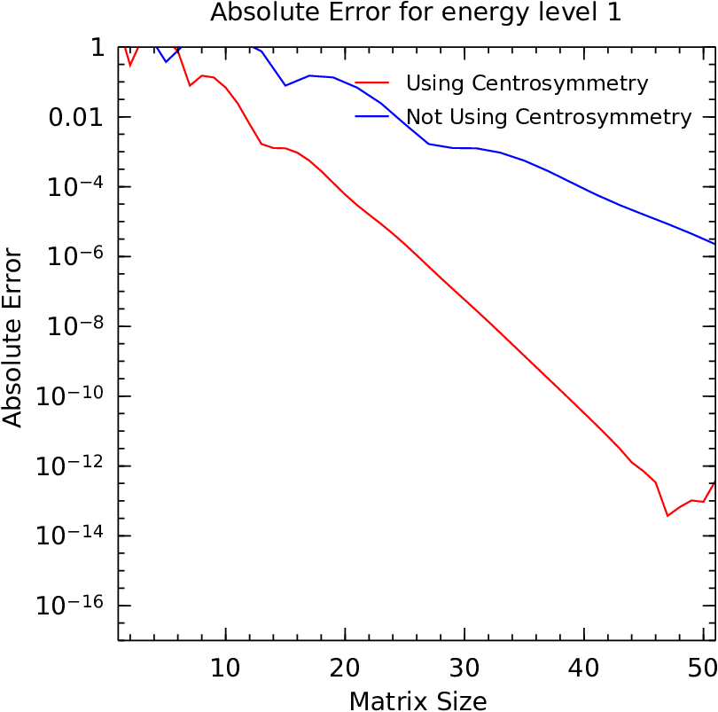
Figure 1 presents the absolute error between our approximation and the exact values given in (48). The absolute error is defined by:

$${\rm Absolute\,\,error}=\left|\mathcal{E}_{l}(N)-{\rm Exact\,\,value}\right|\qquad\textrm{for}\qquad l=0,1.$$

(49)

The optimal mesh size obtained in [10]:

$$h=\dfrac{W\left(\frac{2^{m}\pi^{2}(m+1)N}{\sqrt{c_{m}}}\right)}{(m+1)N},$$

(50)

where $W(x)$ is the Lambert W function, is used in the calculation.

As can be seen from Figure 1, using the centrosymmetric property improves the convergence rate of the DESCM significantly.

Sturm-Liouville eigenvalue problems are abundant in scientific and engineering problems. In certain applications, these problems possess a symmetry structure which results in the Sturm-Liouville operator to be commutative with the parity operator. As was proven in Theorem 3.5, applying the DESCM will preserve this symmetry and results in a generalized eigenvalue problem where the matrices are symmetric centrosymmetric. The centrosymmetric property leads to a substantial reduction in the computational cost when computing the eigenvalues by splitting the original eigenvalue problem of dimension $(2N+1)\times(2N+1)$ into two smaller generalized eigensystems of dimension $N\times N$ and $(N+1)\times(N+1)$. Moreover, due to the internal block structure of the matrices obtained using the DESCM, we have shown that only $\dfrac{1}{N+1}$ of all entries need to be computed and stored at every iteration in order to find all of their eigenvalues. Numerical results are presented for the time independent Schrödinger equation (42) with an anharmonic oscillator potential (43). Four exact potentials with known eigenvalues are tested and the results clearly demonstrated the reduction in complexity and increase in convergence.

References

- [1] A. Zettl. Sturm-Liouville Theory. Birkhäuser-Verlag, Basel, 2005.
- [2] W. Auzinger, E. Karner, O. Koch, and E. Weinmüller. Collocation methods for the solution of eigenvalue problems for singular ordinary differential equations. Opuscula Mathematica, 26(2):229–241, 2006.
- [3] B. Chanane. Computing the eigenvalues of singular Sturm-Liouville problems using the regularized sampling method. Applied Mathematics and Computation, 184(2):972–978, 2007.
- [4] M.M. Tharwat, A.H. Bhrawy, and A. Yildirim. Numerical computation of eigenvalues of discontinuous Sturm-Liouville problems with parameter dependent boundary conditions using sinc method. Numerical Algorithms, 63(1):27–48, 2013.
- [5] M.M. Tharwat. Sinc approximation of eigenvalues of Sturm-Liouville problems with a Gaussian multiplier. Calcolo, 51(3):465–484, 2013.
- [6] M. Jarratt, J. Lund, and K.L. Bowers. Galerkin schemes and the Sinc-Galerkin method for singular Sturm-Liouville problems. Journal of Computational Physics, 89(1):41–62, 1990.
- [7] F. Stenger. Numerical Methods Based on Whittaker Cardinal, or Sinc Functions. SIAM Review, 23(2):165–224, 1981.
- [8] F. Stenger. Summary of sinc numerical methods. Journal of Computational and Applied Mathematics, 121(1-2):379–420, 2000.
- [9] P. Gaudreau, R. Slevinsky, and H. Safouhi. The double exponential sinc collocation method for singular sturm-liouville problems. arXiv:1409.7471.
- [10] P. Gaudreau, R. Slevinsky, and H. Safouhi. The double exponential sinc-collocation method for computing energy levels of anharmonic oscillators. Annals of Physics, 360:520–538, 2015.
- [11] E. Saibel. Note on the Inversion of a Centrosymmetric Matrix. The American Mathematical Monthly, 49(4):246–248, 1942.
- [12] A. Cantoni and P. Butler. Eigenvalues and eigenvectors of symmetric centrosymmetric matrices. Linear Algebra and its Applications, 13(3):275–288, 1976.
- [13] A.B. Cruse. Some combinatorial properties of centrosymmetric matrices. Linear Algebra and its Applications, 16:65–77, 1977.
- [14] A. Lee. Centrohermitian and skew-centrohermitian matrices. Linear Algebra and its Applications, 29:205–210, 1980.
- [15] J.L. Stuart. Matrices that Commute with a Permutation Matrix. SIAM Journal on Matrix Analysis and Applications, 9:408–418, 1988.
- [16] R.D. Hill, R.G. Bates, and S.R. Waters. On Centrohermitian Matrices. SIAM Journal on Matrix Analysis and Applications, 11(1):128–133, 1990.
- [17] N. Muthiyalu and S. Usha. Eigenvalues of centrosymmetric matrices. Computing, 48(2):213–218, 1992.
- [18] D.A. Nield. Odd-Even Factorization Results for Eigenvalue Problems. SIAM Review, 36(4):649–651, 1994.
- [19] A. Melman. Symmetric centrosymmetric matrix-vector multiplication. Linear Algebra and its Applications, 320(1-3):193–198, 2000.
- [20] D. Tao and M. Yasuda. A spectral characterization of generalized real symmetric centrosymmetric and generalized real symmetric skew-centrosymmetric matrices. SIAM Journal on Matrix Analysis and Applications, 23(3):885–895, 2002.
- [21] T.T. Lu and S.H. Shiou. Inverses of 2 X 2 block matrices. Computers and Mathematics with Applications, 43:119–129, 2002.
- [22] I.T. Abu-jeib. Centrosymmetric matrices: properties and an alternative approach. Canadian Applied Mathematics Quarterly, 10(4):429–445, 2002.
- [23] F.Z. Zhou, X.Y. Hu, and L. Zhang. The solvability conditions for the inverse eigenvalue problems of centro-symmetric matrices. Linear Algebra and Its Applications, 364:147–160, 2003.
- [24] F.Z. Zhou, L. Zhang, and X.Y. Hu. Least-square solutions for inverse problems of centrosymmetric matrices. Computers and Mathematics with Applications, 45(10-11):1581–1589, 2003.
- [25] Z.Y. Liu. Some properties of centrosymmetric matrices. Applied Mathematics and Computation, 141(2-3):297–306, 2003.
- [26] H. Fassbender and K.D. Ikramov. Computing matrix-vector products with centrosymmetric and centrohermitian matrices. Linear Algebra and Its Applications, 364:235–241, 2003.
- [27] W.F. Trench. Characterization and properties of matrices with generalized symmetry or skew symmetry. Linear Algebra and Its Applications, 377:207–218, 2004.
- [28] W.F. Trench. Inverse eigenproblems and associated approximation problems for matrices with generalized symmetry or skew symmetry. Linear Algebra and Its Applications, 380:199–211, 2004.
- [29] L. Zhongyun. Some properties of centrosymmetric matrices and its applications. Numerical Mathematics, 14(2):297–306, 2005.
- [30] Z.Y. Liu, H.D. Cao, and H.J. Chen. A note on computing matrix-vector products with generalized centrosymmetric (centrohermitian) matrices. Applied Mathematics and Computation, 169(04):1332–1345, 2005.
- [31] Z. Tian and C. Gu. The iterative methods for centrosymmetric matrices. Applied Mathematics and Computation, 187(2):902–911, 2007.
- [32] H. Li, D. Zhao, F. Dai, and D. Su. On the spectral radius of a nonnegative centrosymmetric matrix. Applied Mathematics and Computation, 218(9):4962–4966, 2012.
- [33] M. El-Mikkawy and F. Atlan. On solving centrosymmetric linear systems. Applied Mathematics, 04(12):21–32, 2013.
- [34] P. Gaudreau, R.M. Slevinsky, and H. Safouhi. The Double Exponential Sinc Collocation Method for Singular Sturm-Liouville Problems. arXiv:1409.7471v2, 2014.
- [35] N. Eggert, M. Jarratt, and J. Lund. Sinc function computation of the eigenvalues of Sturm-Liouville problems. Journal of Computational Physics, 69(1):209–229, 1987.
- [36] M. Mori and M. Sugihara. The double-exponential transformation in numerical analysis. Journal of Computational and Applied Mathematics, 127(1-2):287–296, January 2001.
- [37] F. Stenger. Matrices of Sinc methods. Journal of Computational and Applied Mathematics, 86(1):297–310, 1997.
- [38] B.H. Bransden and C.J. Joachain. Quantum Mechanics. Pearson Prentice Hall, Essex, UK, 2nd edition, 2000.
- [39] J.R. Weaver. Centrosymmetric (Cross-Symmetric) Matrices, Their Basic Properties, Eigenvalues, and Eigenvectors. The American Mathematical Monthly, 92(10):711–717, 1985.
- [40] R.N. Chaudhuri and M. Mondal. Improved Hill determinant method: General approach to the solution of quantum anharmonic oscillators. Physical Review A, 43(7):3241–3246, 1991.