Active skeleton for bacteria modeling
Abstract
The investigation of spatio-temporal dynamics of bacterial cells and their molecular components requires automated image analysis tools to track cell shape properties and molecular component locations inside the cells. In the study of bacteria aging, the molecular components of interest are protein aggregates accumulated near bacteria boundaries. This particular location makes very ambiguous the correspondence between aggregates and cells, since computing accurately bacteria boundaries in phase-contrast time-lapse imaging is a challenging task. This paper proposes an active skeleton formulation for bacteria modeling which provides several advantages: an easy computation of shape properties (perimeter, length, thickness, orientation), an improved boundary accuracy in noisy images, and a natural bacteria-centered coordinate system that permits the intrinsic location of molecular components inside the cell. Starting from an initial skeleton estimate, the medial axis of the bacterium is obtained by minimizing an energy function which incorporates bacteria shape constraints. Experimental results on biological images and comparative evaluation of the performances validate the proposed approach for modeling cigar-shaped bacteria like Escherichia coli. The Image-J plugin of the proposed method can be found online at http://fluobactracker.inrialpes.fr.
keywords
bacteria modeling; medial axis; active contours; active skeleton; shape contraints.1 Introduction
One of the fundamental issues addressed by Computational Cell Biology is the characterization of spatio-temporal dynamics of bacterial cells and their molecular components (Slepchenko, Schaff, et al., 2002). The rapid development of techniques for fluorescence imaging in recent years has opened new research opportunities, that need to cope with the availability of automated image analysis tools to be fully exploited. In the study of E. Coli aging (Lindner, Madden, et al., 2008), the molecular components of interest are protein aggregates accumulated at the old pole region of the aging bacterium. These subcellular components, visualized by fluorescence imaging techniques, need to be reliably associated to their host cells, which are generally visualized with phase-contrast microscopy. Figure 1 shows a pair of simultaneous frames extracted from a time-lapse phase-contrast and fluorescence image sequence. The automatic association between aggregates and bacteria requires a very accurate estimation of bacteria boundaries in this case, because aggregates accumulate near these boundaries (see Figure 2). In addition to boundary accuracy, a requirement for bacteria modeling is the possibility to derive accurate cell measurements such as length, width, orientation, perimeter, etc., that are fundamental characteristics of bacteria (Osborn and Rothfield, 2007). For instance, in bacteria like E. Coli, tracking population variability over time helps to understand the combinations of effects of genetic and environmental factors on cell phenotype. Finally, having the possibility to describe the location of subcellular components in an intrinsic cell-centered coordinate system may be very useful to characterize intracellular dynamics (Coquel, Jacob, et al., 2013).


This paper aims to provide an algorithm able to extract from an image a complete parametric description of cigar- or rod-shaped bacteria (e.g., E. coli) that it contains. The underlying mathematical representation is a curvilinear skeleton (also called medial axis), which defines, after an appropriate (non-constant) dilation, the boundary of the bacterium. This model is built by evolving a first skeleton estimate so as to minimize an energy that promotes a good image fitting while enforcing the expected properties of the cell shape. In the following, we present the state of the art related to the use of skeletons for shape characterization and active contours, on which the proposed model relies.
1.1 Background
Segmentation, the task of partitioning an image into coherent regions, is ill-posed and simple continuity or homogeneity assumptions cannot cope with the large variability of object appearances. In some specific applications for which one expects to see objects from a particular class, prior knowledge (e.g., clues on appearance or shape) may be exploited to reduce the space of variations. Such cues have traditionally been used by the Computer Vision community for object recognition, but their usefulness in segmentation has only more recently reached a common consensus (Leibe, Leonardis and Schiele, 2006). Appearance-based methods rely on features points as Scale-Invariant Feature Transform (SIFT) (Lowe, 2001) but their efficiency has proved to be limited since in general, object identity is more a function of form that a function of appearance (Siddiqi, Kimia, et al., 2001; Siddiqi and Kimia, 1996; Siddiqi and Kimia, 1995; Leordeanu, Hebert and Sukthankar, 2007). Furthermore, in applications such as living cell imaging, where the intensities are reduced to a minimum to avoid photodamage and photobleaching, key features may not be sufficiently available.
In the use of shape as an alternative or to reinforce the use of appearance, the skeleton, defined by Blum (Blum, 1973) as the set of medial loci of the maximal disks contained inside the object, has received much attention in the literature (Bai and Latecki, 2008; Siddiqi, Shokoufandeh, et al., 1998; Zhu and Yuille, 1995). Compared to other shape representation such as edge fragments and shock graphs, the skeleton offers more flexibility in modeling spatial relationships between parts and has a good repeatability/distinctiveness trade-off. Although its usefulness for shape matching and classification on silhouettes has been recognized since the nineties, it is only recently that skeletons have been exploited for non-rigid object detection (Bai, Wang, et al., 2009; Trinh and Kimia, 2011). In all these methods, the object is first recognized using reference skeletons, and then the skeleton is used to optimize an initial segmentation.
The idea of optimizing an initial segmentation, under some constraints, is at the core of active contour (also called snakes) methods, which specifically refine an initial approximate contour according to the image data. Early active contour models (Kass, Witkin and Terzopoulos, 1988; Osher and Sethian, 1988; Cohen, 1992; Caselles, Catté, et al., 1993) act by minimizing an energy function consisting of a data term (including image information), and a regularization term which, in general, imposes smoothness constraints on the object shape. According to the nature of the image information included in the data term, the existing active contour methods can be categorized into two types: edge-based models and region-based models. Edge-based models use local image information —typically, gradient information— (Kass, Witkin and Terzopoulos, 1988; Staib and Duncan, 1992; Park, Schoepflin and Kim, 2001) to stop the contour evolution on the object boundary, while region-based approaches (Cohen, Bardinet and Ayache, 1992; Ivins and Porrill, 1995; Zhu and Yuille, 1996; Chesnaud, Refregier and Boulet, 1999; Chan and Vese, 2001; Jehan-Besson, Gastaud, et al., 2003; Zhang, Zhang, et al., 2010) use global image features inside and outside the contour to control the evolution. Region-based methods relying on local information are able to segment images with non-homogeneous intensities (Li, Kao, et al., 2007; Li, Kao, et al., 2008). However, as detailed by Wang et al. (Wang, Li, et al., 2009), such localization property introduces many local minima of the nonconvex energy functional. Consequently, the result is more dependent on the initialization of the contour. The initialization issue itself is since long time the object of investigations (Cohen, 1991; Cohen and Cohen, 1993; Kass, Witkin and Terzopoulos, 1988; Bajcsy and Kovacic, 1989; Jain, Zhong and Dubuisson-Jolly, 1998; Cohen and Kimmel, 1997; Amini, Weymouth and Jain, 1990; Geiger, Gupta, et al., 1995) and, recently, it has been partially addressed by the formulation of convex energy functionals (Mao, Liu and Shi, 2010; Thieu, Luong, et al., 2011), for which a single global minimum exists. According to the contour parametrization method used to model the smoothness constraint included in the regularization term, the existing active contour methods can be categorized into three classes: level sets snakes (Osher and Sethian, 1988; Caselles, Catté, et al., 1993; Malladi, Sethian and Vemuri, 1995), point-based snakes (Kass, Witkin and Terzopoulos, 1988; Xu and Prince, 1998) and parametric snakes (Staib and Duncan, 1992; Brigger, Hoeg and Unser, 2000). Level sets define the 2D-curve implicitly from an evolving surface in a 3D space. They easily enable topology changes but are computationally expensive. The smoothness constraints are also implicit, that is, they are defined on the surface and not on the curve. Point-based snakes correspond to no parametrization or equivalently to a polygonal line (B-splines of degree zero). Parametric snakes define the curve between knot points (Brigger, Hoeg and Unser, 2000; Jacob, Blu and Unser, 2004) via a basis decomposition such as B-splines (Marc, Menet and Medioni, 1990; Brigger, Hoeg and Unser, 2000) or Fourier exponentials (Staib and Duncan, 1992). The overall smoothness is ensured with curvature and eventually length minimization. When a shape-prior is introduced into point-based or parametric snakes, a deformable template model is obtained (Jain, Zhong and Dubuisson-Jolly, 1998). The prior shape model may be built ad hoc with analytical formulas (Widrow, 1973; Yuille, Hallinan and Cohen, 1992; Jolly, Lakshmanan and Jain, 1996; Lakshmanan and Grimmer, 1996) or derived from a training set (Staib and Duncan, 1992; Cootes, Hill, et al., 1993; Cootes, Taylor, et al., 1995; Cootes and Taylor, 1995; Davatzikos, Tao and Shen, 2003). For analytic models, the shape deformations are given by the model parameters (e.g., slope for straight lines, radius for circles). Mostly no probability distribution is needed. Training methods, usually called active shape models (Staib and Duncan, 1992; Cootes and Taylor, 1995; Davatzikos, Tao and Shen, 2003), are more flexible since they can be applied easily to any reproducible shape. However, they require to define an average shape and deformation models, which could bias the result if, for example, the training set is too small.
1.2 Active skeleton
Instead of matching a given bacteria template to a previously computed edge map as in classical recognition problems, or evolving an initial contour toward the object outline as in classical active-contour methods, we propose an active skeleton model which evolves initial skeletal polygonal lines toward the true medial axes of the bacteria. The advantage of the proposed approach for segmentation is that it allows to introduce strong shape constraints adapted to the bacteria class (here, cigar-shaped bacteria), which improves the accuracy of the boundary location even in very noised images.
The paper is organized as follows. In Section 2, we describe the skeletal model we are considering, while Section 2.4 details the active skeleton initiation and the evolution process based on a variational (energy minimization) formulation. Section 3 provides results and comparisons to other segmentation methods.
2 Method
2.1 Skeleton model
We model a digital image acquired by a contrast-phase microscopy as a real valued discrete function , where is a rectangle.
Definition 1.
A ball centered at and having radius is a maximal disk of a shape if and
We denote the maximal disks of a shape by the symbol .
Definition 2.
The morphological skeleton of a bacterium on the image is the set of maximal disks centers of .
We represent a skeleton by an ordered set of points with associated radius value: , where represents the center of the maximal disk of radius . The skeleton is hence composed of segments , with . Given the skeleton , the bacterium is built up by dilating the centers of the maximal disks according to their associated radius, which is linearly interpolated inside each segment. Let a segment of the skeleton, then for each point of , the corresponding radius is computed as a linear interpolation of and : , with .
Given an initial skeleton, the optimization of its location strongly depends on the underlying segment dilations and in turn to the definition of distance used for the dilation. In the following, we define two distance models and, according to them, we derive the expression of the dilation models.
2.2 Distance models
In this section, we first define a simplified model of distance of a point to a segment, say , and then we define an accurate orientation based distance, say , that takes the radii difference into account.
Definition 3.
Simplified distance of a point to a segment. Let be any point of the image and any segment of the skeleton. Denoting by the projection of on the line through and , can be written as , with . The simplified Euclidean-based distance of a point to a segment is defined as follows.
| (2.1) |
where is the Euclidean norm. In Fig.3 (up) it can be observed that the distance coincides with the Euclidean distance between two points only if the orthogonal projection of on the line through and lies on the segment .
The value of can be computed from the scalar product : , where , , and (the length of segment ). If the orthogonal projection of on lies on , then the distance of to coincides to the distance of to . In this case, such a distance can be written as . By introducing :
| (2.2) |
the simplified distance from any point to a segment can be written as: .
Definition 4.
Orientation-based distance of a point to a segment.
Let be any point of the image and any segment of the skeleton. Let be the difference between the radii value associated to the extremities of the segment and the segment length.
- •
Case 1: : let be the common tangent to the circles with centers and radii respectively, lying on the same half-plane than compared to . Let be the orthogonal projection of over , and the intersection of the line through and with the line through and . Writing as , with , the orientation-based distance is defined as follows: (see figure 3 (down)):
where is the euclidean norm.
- •
Case 2: :
Under the assumption , with . Let such that . Then one has simply to replace with in the equations derived for the simplified distance.


To explicit , one can compute the angle between and according to . It comes that
| (2.3) |
Note again that is an algebraic value. To deal with the case one can extend the definition of , for example in the following manner:
| (2.4) |
Now one can compute in any case . Because of the restrictions of , the definition can be extended as:
| (2.5) |
Finally, the general expression of is as follows:
| (2.6) |
2.3 Dilation models
Before introducing the dilations models derived from the above definitions of distance, we define the distance of a point to as skeleton.
Definition 5.
Distance of a point to a skeleton. Let a skeleton on the image and a point of .
Definition 6.
Dilation model derived from the simplified distance of a point to a segment. Let a skeleton and a segment of . For any point , let the segment that has minimal simplified distance from . The simplified dilation of is given by the set of points such that their simplified distance to is inside the maximal disks with interpolated radius: where is defined in equation 2.2
Definition 7.
Dilation model derived from orientation-based distance of a point to a segment. Let a skeleton and the segment of . For any point , let . The orientation-based dilation of is:
where is defined in equation 2.5.

Denoting by and the dilations obtained by using the distances and respectively, as it can be observed on the cartoon example shown in Fig. 4: in the region delimited by the vertical dashed green lines, and elsewhere. As it can be appreciated, the dilated models differ slightly even if the difference between the radii is large. Since bacteria width has low variations, radii difference values are generally small compared to the segment length. Hence, the difference between the dilation models would be not significant. Additionally, when using the simplified distance, the corresponding dilation contains less derivative terms and discontinuities, and consequently the variational optimization based on it would be computationally faster and more stable numerically. Hereafter, to simplify the notations, we will use the symbol to denote either or , and to denote either or according to the desired distance model.
General remarks
Although the distances and are continuous, both dilation outlines are made up of arc circles and straight lines. Note that the scale parameter of the outline is contained in the radius values: big or small outlines may be described with the same skeleton. Furthermore, some measures of interest inherent to the bacteria class are immediate with this representation: orientation, thickness, perimeter and length.
2.4 Active skeletons
2.4.1 Skeleton initialization
The optimization process relies on the availability of an initial skeleton for each bacterium. In this work, we derived it from the closed contours obtained by applying the bacteria segmentation method proposed in Primet, Demarez, et al. (2008). After computing the morphological skeleton through the use of morphological operators, a linear vectorization is performed by using an iterative method inspired to Wall and Danielsson (1984); Potier and Vercken (1994) but based on angle variations. The vectorization starts from the farthest point from the gravity center of the skeleton. To take into account the presence of possible holes, a spline-interpolation is used to build a continuous skeletal line, which is finally sampled uniformly according to the wished accuracy of the skeleton.
2.4.2 Skeleton optimization
Given an image and the initial skeleton approximations , the aim of the active skeleton model is to find the skeletons corresponding to the true medial axis of bacteria by evolving the initial skeletons. This is achieved by minimizing an energy function made up of two terms: a data-fidelity term and a regularity term that incorporates bacteria shape constraints. To handle the specific issue of several non-ovelapping objects, we propose an additional repulsion energy term.

Data term
Images captured by a phase-contrast microscopy are characterized by a difference of contrast between the foreground specimen and the background. Therefore, the data term has to be small when the difference of the contrast between foreground and background is large. Since time-lapse imaging objects contours may have large and slow variations (that is, strong low-frequency components), the use of a local neighborhood allows us to have a reasonable local model of the background. Typically, the data term corresponds to the difference between the average intensity inside the closed contour, and the average intensity in a ring surrounding it that corresponds to a high contrast between a bacterium and its local background. Since the objective function to be minimized has to be differentiable, the spatial condition is expressed through a smooth pixel selection function .
| (2.7) |
The data term is expressed as the difference between the internal energy and the external energy , which are defined as follows
| (2.8) |
where is an increasing smooth contrast function allowing to adapt the imaging contrast to the data, is the width of the ring surrounding the closed contours and, since can be written as , . It is easy to see that selects pixels inside the closed contour, whereas selects outside pixels.
Regularity terms
Two regularity assumptions are embedded into the energy function by imposing a smooth segment angle variation and radii homogeneity.
Most of the bacteria are weakly bent, therefore the skeleton curvature has to be as small as possible. The discrete curvature at point is measured by the angle of the arc at , that corresponds to the angle . Numerically, we compute . The corresponding curvature-related regularization term is:
| (2.9) |
Since the bacterium thickness is quite homogeneous, the difference between the radii of the skeleton points, , should be small. We consider the median radius value defined as . The corresponding energy term is
| (2.10) |
Repulsion term
An additional repulsion term may be added when dealing with bacteria colonies. Denoting by the distance between a point and the skeleton , the corresponding distance between and the bacteria is , where is the interpolated radius from when computing the distance . Since has to be avoided, by defining a repulsion function minimal when , the repulsion energy term can be written as:
| (2.11) |
Overall energy
The global energy to minimize combines all above energy terms: , where are positive weights. The energy minimization requires to compute derivatives according to points coordinates and radii. All derivatives are given in Appendix.
3 Results
The parameters defined in last section - , , , , , the contrast function and the repulsion funcion - were set once for all when correctly calibrated on our dataset. The experimental values were: , , , , thickness pixels. The contrast function we used is , which enhances the contrast between inside and outside mean values of bacteria. We have chosen a quadratic repulsion function to penalize bigger overlaps:
| (3.1) |
with pixels. The algorithm was implemented in C with the MegaWave2 library 11 1 The software in C will be made publicly available with the publication of the article.
3.1 Method validation

In this section, we compare our active skeleton model to the active contour model by using the Haussdorff distance to a synthetically generated ground truth on a set of synthetically generated images. Since both methods require a rough initialization we drew it by hand. To generate the ground truth, as well as the test data, we started by considering a bacterial colony phase-contrast image. First, we computed the bacteria skeletons by applying the proposed method and then, by relying on the skeletons obtained, we recovered a synthetic image by computing each pixel value as
| (3.2) |
where is the distance of the pixel to the segment of a skeleton having as extremities the pixels and with associated radii and respectively (see Fig. 6). is the Gauss error function and is the interpolated radium computed on the projection of on ( in Fig. 6). The interpolated radium value is computed as: with .

As test data, we used noised versions of the so generated synthetic image (see Figure 7), obtained by adding a Gaussian white noise with increasing standard deviations. As ground truth, we used the boundaries from which the synthetic image has been generated. This is justified by the fact that, on the unnoised synthetic image, the average Haussdorff distances to ground truth of both methods are almost the same and of less than 1/10 of pixel (see Fig. 8) for a standard deviation of noise equal to zero.


Fig. 8 shows the Haussdorff distance to the ground truth of the active skeleton and the active contour methods. Since the active contour model assumes that the object contours are smooth, we previously smoothed the image by using a Gaussian kernel of standard deviation before applying this method. As it is shown in Fig.9, for relatively small values of the standard deviation of the Gaussian smoothing kernel, the performances of the active contour method slightly improves, since the ”edgness” of curves is enhanced by smoothing. However, there is an upper bound to the level of smoothing that can be applied which is related to the scale of the image structure we are looking for. The proposed active skeleton model allows to enforce smoothness without becoming excessively sensitive to noise by integrating an a priori on the shape which is itself smooth (rod or cigar-shape). It is worth to remark that on real images, the image contrast across cells boundaries is not constant as it is for our data test images. This greatly deteriorates the performances of the active contour method as it can be appreciated in Fig. 10. This Fig. shows the interest of the proposed method in determining the association cell-aggregate. As detailed in section 1, solving this association requires accurate boundary estimation since fluorescent molecular components are usually concentrated at the poles of bacteria.


3.2 Application to the study of Escherichia Coli aging


 |
 |
| (a) | (b) |
 |
 |
| (c) | (d) |
 |
 |
| (e) | (f) |
In Escherichia coli (E. coli) bacteria, aging-related protein aggregates accumulate at the old pole region of the aging bacterium. Studying the dynamics of these molecular components inside the cells requires automatic tools for 1) detecting protein aggregates in fluorescence images, 2) computing bacteria boundaries in the corresponding contrast-phase image, 3) assigning each protein aggregate to one cell, 4) expressing the coordinates of the protein aggregates in the basis composed of the cell long (the median line) and short axes (along the skeleton width). We used the method in Dimiccoli, Jacob and Moisan (2015) to detect protein aggregates in fluorescence images, the method Primet, Demarez, et al. (2008) for segmenting the cells in contrast-phase images, and the active skeleton method to refine bacteria boundaries prior to the affiliation of protein aggregates to cells. Then the final skeletons were used in two different manners. Firstly, to localize the protein aggregates in the skeletal short and long axes referential. Then, the simple shape of the skeleton was used to estimate the total cell width and length as that of the respective skeleton.
As a convention, we refer below to the aggregate coordinate along the long axis as the x-coordinate and that along the short axis as the y-coordinate (see Fig. 11 (a)). In Fig. 11 (b) is shown the histogram of the component computed over 1,644 images. It can be seen that most aggregates accumulate along the center, that undergoes division, and the poles of bacteria. Fig. 12 schematizes the increase of the cell half-length during growth that dominates the movement along the x-axis, also showing the time evolution of the mean displacement.
4 Discussion
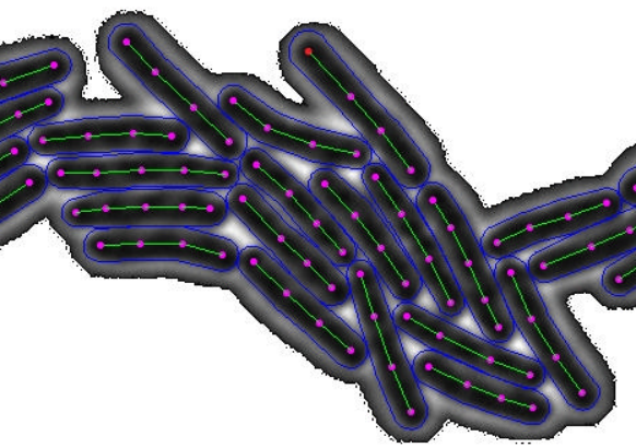
This study has covered a number of aspects of the problem of investigating the dynamics of bacteria cells and their molecular components. Overall the work reported produced numerical values for validation results and experimental results, and the discussion will be organised to highlight different parts of the process and to analyse the computational complexity. We will end this section by discussing the range of applicability of the proposed method. An example of initialization is shown on figure 13 (a): we choose a default number of four points per bacteria (and more if the spline interpolation is too far from the skeleton). Even if the morphological skeleton provides radii values at each skeleton point, we used a constant value corresponding to the minimal contact radius instead (see blue outlines). In this way, the influence of the initial segmentation obtained by applying the method proposed by Primet el al. Primet, Demarez, et al. (2008) is minimized. The results correspond to what is expected: the different final skeletons are inside the bacteria and the implicit outlines demarcate dark areas from light outsides. Figures 13 (b) and 13 (c) show final states from initial positions given in figure 13 (a). They highlight the interest of the repulsion energy . The second segmentation seems fully coherent with the initial image.
From a biological point of view the segmented bacteria are too thin since they should be in contact according to the experimental conditions. Of course this is not the case for the above segmentation (e.g on figure 13 (c)) because we consider that there are bright pixels outside: the bright pixels isolate the bacteria from each other. For this experimental reason, the bacteria have to be enlarged in some way. We propose two strategies to fix this problem. The first solution consists in adding a positive coefficient in the expression . This enables one to enlarge the bacteria according to the luminosity transitions as shown on figure 13 (d). Though theoretically this is a good solution, the result is that different bacteria are more ore less dilated according to their outline intensity. Moreover, when taking low values of (very big bacteria) the active skeleton may leak in the background. Another repulsion term from the bottom could be introduced but it supposes to set an additional arbitrary parameter: the minimal distance of bacteria to the bottom . Then the result is biased like on red dots in Fig. 13 (e). For the biological study we prefer another solution. We consider that bacteria are bigger than they appear on the image. Then the optimization is done by considering bigger bacteria in the repulsion energy term (interaction between real bacteria) while having a thin eroded representation of bacteria for the data confidence energy . In other words, we assume that an eroded representation of the bacteria may fit the image. Let us call the radius difference between real and thin bacteria. To adapt consequently the repulsion term , in equation (3.1) is replaced by to prevent the overlapping of the physical bacteria. The optimization process produces thin bacteria. Then to obtain the physical bacteria from their thin image version, a homogeneous dilation is performed after the optimization. In practice, it simply consists in adding to all values. Figure 13 (f) presents a pixels thickness difference.
The computational complexity of the proposed method depends on three parameters: the number of active skeletons, the number of skeletal points used to model each of them and the image resolution. More precisely, for one step of the gradient descent and for a single skeleton, the complexity of deriving the energy term is , where is the number of skeleton points and is the number of pixels within a box surrounding the skeleton dilation. For skeletons without repulsion energy, the complexity is . When considering the repulsion energy, it becomes , where the second term corresponds to inter-bacteria distances. Since accurate segmentation of bacteria can be achieved with a few skeletal points, the algorithm complexity will mainly depend on the image resolution and on the number of bacteria in this particular application.
We conclude by remarking that although this work was tailored to cigar- or rod-shaped bacteria, it would work as well for any kind of curved ovoid shape. For non-ovoid shapes, it could be adapted by changing the dilation model. For more complicated ramified shapes, the skeleton model itself should be adapted. The utility spectra of the proposed method is not restricted to bacteria, but to all cases in which a precise segmentation of cigar- or rod-shaped object is needed and the image quality is poor. For instance it could be very useful for segmenting images of insects in the study of insect populations, or for the segmentation and recognition of tumors and cigar- or rod-shaped cells.
5 Conclusions
This paper has proposed an active skeleton approach for bacteria modeling, that presents several advantages for the study of bacteria shape properties and the dynamics of their molecular components. Indeed, the long and short axis of the skeleton define a reference system centered to the bacterium, which is crucial to study the dynamics of subcellular components inside the cell. In addition, the computation of shape properties such as local orientation, thickness, length and perimeter from the skeleton representation is straightforward. Finally, bacteria boundaries are computed accurately even in very noised images by introducing implicitly smooth shape priors into the segmentation process. The improved accuracy is important to reduce the ambiguity of the association molecule/cell in time-lapse fluorescence and phase-contrast imaging.
The proposed model has been successfully used to study the dynamic of protein aggregates in E. Coli Coquel, Jacob, et al. (2013). Localization of proteins to specific positions inside bacteria is crucial to several physiological processes, including chromosome organization, chemotaxis or cell division and aging. The Image-J plugin of the proposed method can be found online at http://fluobactracker.inrialpes.fr.
Further improvements could be discussed and developed according to the kind of data and to the imaging task to deal with. For example, the fidelity term of the energy functional could be chosen differently from the literature on data energy terms for snakes. Ad-hoc initializations could be derived from morphological gray-level skeletons and segment extraction. Finally, the skeleton model could handle more complex shapes, with more branches and angle constraints, and eventually with other distance definitions relaxing the circular extremity of each branch.
Acknowledgement
This work has been partially supported by the project PAGDEG: Causes and consequences of protein aggregation in cellular degeneration. Funding: French ANR. The authors would like to thank Anne-Sophie Coquel for sharing the biological data and contributing to validate the proposed method.
References
- Amini, Weymouth and Jain (1990) Amini A, Weymouth T, Jain R. 1990. Using dynamic programming for solving variational problems in vision. IEEE Transactions on pattern analysis and machine intelligence:855–867.
- Bai and Latecki (2008) Bai X, Latecki LJ. 2008. Path Similarity Skeleton Graph Matching. Pattern Analysis and Machine Intelligence, IEEE Transactions on. 30(7):1282–1292.
- Bai, Wang, et al. (2009) Bai X, Wang X, Latecki LJ, Liu W, Tu Z. 2009. Active skeleton for non-rigid object detection. In: Computer Vision, 2009 IEEE 12th International Conference on; Sep.; Kyoto. IEEE; p. 575–582.
- Bajcsy and Kovacic (1989) Bajcsy R, Kovacic S. 1989. Multiresolution elastic matching. Computer Vision, Graphics, and Image Processing. 46(1):1–2.
- Blum (1973) Blum H. 1973. Biological shape and visual science (part I). Journal of Theoretical Biology. 38(2):205–287.
- Brigger, Hoeg and Unser (2000) Brigger P, Hoeg J, Unser M. 2000. B-spline snakes: a flexible tool for parametric contour detection. IEEE Transactions on Image Processing. 9(9):1484–1496.
- Caselles, Catté, et al. (1993) Caselles V, Catté F, Coll T, Dibos F. 1993. A geometric model for active contours in image processing. Numerische Mathematik. 66(1):1–31.
- Chan and Vese (2001) Chan T, Vese L. 2001. Active contours without edges. IEEE Transactions on image processing. 10(2):266–277.
- Chesnaud, Refregier and Boulet (1999) Chesnaud C, Refregier P, Boulet V. 1999. Statistical region snake-based segmentation adapted to differentphysical noise models. IEEE Transactions on Pattern Analysis and Machine Intelligence. 21(11):1145–1157.
- Cohen, Bardinet and Ayache (1992) Cohen L, Bardinet E, Ayache N. 1992. Surface reconstruction using active contour models. Report INRIA.
- Cohen and Cohen (1993) Cohen L, Cohen I. 1993. Finite-element methods for active contour models and balloons for 2-D and 3-D images. IEEE Transactions on Pattern Analysis and Machine Intelligence. 15(11):1131–1147.
- Cohen and Kimmel (1997) Cohen L, Kimmel R. 1997. Global minimum for active contour models: A minimal path approach. International Journal of Computer Vision. 24(1):57–78.
- Cohen (1991) Cohen LD. 1991. On active contour models and balloons. CVGIP: Image Underst. 53(2):211–218.
- Cohen (1992) Cohen LD. 1992. On active contour models. Springer Verlag.
- Cootes, Hill, et al. (1993) Cootes T, Hill A, Taylor C, Haslam J. 1993. The use of active shape models for locating structures in medical images. In: Information Processing in Medical Imaging. Springer; p. 33–47.
- Cootes and Taylor (1995) Cootes T, Taylor C. 1995. Combining point distribution models with shape models based on finite element analysis. Image and Vision Computing. 13(5):403–409.
- Cootes, Taylor, et al. (1995) Cootes T, Taylor C, Cooper D, Graham J, et al. 1995. Active shape models-their training and application. Computer vision and image understanding. 61(1):38–59.
- Coquel, Jacob, et al. (2013) Coquel A, Jacob J, Primet M, Demarez A, Dimiccoli M, Julou T, Moisan L, AB L. 2013. Localization of Protein Aggregation in Escherichia coli Is Governed by Diffusion and Nucleoid Macromolecular Crowding Effect. PLoS Comput Biol. 9(4).
- Davatzikos, Tao and Shen (2003) Davatzikos C, Tao X, Shen D. 2003. Hierarchical active shape models, using the wavelet transform. IEEE Transactions on Medical Imaging. 22(3):414–423.
- Dimiccoli, Jacob and Moisan (2015) Dimiccoli M, Jacob JP, Moisan L. 2015. Particle detection and tracking by a-contrario approach: application to fluorescence time-lapse imaging. arXiv preprint arXiv:150706266.
- Geiger, Gupta, et al. (1995) Geiger D, Gupta A, Costa L, Vlontzos J. 1995. Dynamic programming for detecting, tracking, and matchingdeformable contours. IEEE Transactions on Pattern Analysis and Machine Intelligence. 17(3):294–302.
- Ivins and Porrill (1995) Ivins J, Porrill J. 1995. Active region models for segmenting textures and colours. Image and Vision Computing. 13(5):431–438.
- Jacob, Blu and Unser (2004) Jacob M, Blu T, Unser M. 2004. Efficient energies and algorithms for parametric snakes. IEEE Transactions on Image Processing. 13(9):1231–1244.
- Jain, Zhong and Dubuisson-Jolly (1998) Jain A, Zhong Y, Dubuisson-Jolly M. 1998. Deformable template models: A review. Signal Processing. 71(2):109–129.
- Jehan-Besson, Gastaud, et al. (2003) Jehan-Besson S, Gastaud M, Barlaud M, Aubert G. 2003. Region-based active contours using geometrical and statistical features for image segmentation. In: IEEE International Conference in Image Processing; vol. 2. Citeseer; p. 643–646.
- Jolly, Lakshmanan and Jain (1996) Jolly M, Lakshmanan S, Jain A. 1996. Vehicle segmentation and classification using deformable templates. IEEE Transactions on Pattern Analysis and Machine Intelligence. 18(3).
- Kass, Witkin and Terzopoulos (1988) Kass M, Witkin A, Terzopoulos D. 1988. Snakes: Active contour models. International journal of computer vision. 1(4):321–331.
- Lakshmanan and Grimmer (1996) Lakshmanan S, Grimmer D. 1996. A deformable template approach to detecting straight edges in radar images. IEEE Transactions on Pattern Analysis and Machine Intelligence. 18(4):438–443.
- Leibe, Leonardis and Schiele (2006) Leibe B, Leonardis A, Schiele B. 2006. An implicit shape model for combined object categorization and segmentation. Lecture notes in computer science; vol. 4170. Springer Berlin Heidelberg. p. 508–524.
- Leordeanu, Hebert and Sukthankar (2007) Leordeanu M, Hebert M, Sukthankar R. 2007. Beyond local appearance: Category recognition from pairwise interactions of simple features. CVPR.
- Li, Kao, et al. (2008) Li C, Kao CY, Gore J, Ding Z. 2008. Minimization of region-scalable fitting energy for image segmentation. Image Processing, IEEE Transactions on. 17(10):1940–1949.
- Li, Kao, et al. (2007) Li C, Kao CY, Gore JC, Ding Z. 2007. Implicit Active Contours Driven by Local Binary Fitting Energy. In: Computer Vision and Pattern Recognition, 2007. CVPR '07. IEEE Conference on; Jun. IEEE; p. 1–7.
- Lindner, Madden, et al. (2008) Lindner AB, Madden R, Demarez A, Stewart EJ, Taddei F. 2008. Asymmetric segregation of protein aggregates is associated with cellular aging and rejuvenation. Proceedings of the National Academy of Sciences. 105(8):3076–3081.
- Lowe (2001) Lowe DG. 2001. Local feature view clustering for 3D object recognition. In: Computer Vision and Pattern Recognition, 2001. CVPR 2001. Proceedings of the 2001 IEEE Computer Society Conference on; Kauai, HI, USA; vol. 1. Los Alamitos, CA, USA: IEEE; p. I–682–I–688 vol.1.
- Malladi, Sethian and Vemuri (1995) Malladi R, Sethian J, Vemuri B. 1995. Shape modeling with front propagation: A level set approach. IEEE Transactions on Pattern Analysis and Machine Intelligence. 17(2):158–175.
- Mao, Liu and Shi (2010) Mao H, Liu H, Shi P. 2010. A convex neighbor-constrained active contour model for image segmentation. In: Image Processing (ICIP), 2010 17th IEEE International Conference on. IEEE; p. 793–796.
- Marc, Menet and Medioni (1990) Marc P, Menet S, Medioni G. 1990. B-snakes: Implementation and application to stereo. In: IU Workshop. p. 720–726.
- Osborn and Rothfield (2007) Osborn MJ, Rothfield L. 2007. Cell shape determination in Escherichia coli. Current opinion in microbiology. 10(6):606–610.
- Osher and Sethian (1988) Osher S, Sethian J. 1988. Fronts propagating with curvature-dependent speed: algorithms based on Hamilton-Jacobi formulations. Journal of computational physics. 79(1):12–49.
- Park, Schoepflin and Kim (2001) Park H, Schoepflin T, Kim Y. 2001. Active contour model with gradient directional information: Directional snake. IEEE Transactions on Circuits and systems for video technology. 11(2):252–256.
- Potier and Vercken (1994) Potier C, Vercken C. 1994. Modelling digitized graphics. ENST-94-D-012. 94-012.
- Primet, Demarez, et al. (2008) Primet M, Demarez A, Taddei F, Lindner AB, Moisan L. 2008. Tracking of cells in a sequence of images using a low-dimension image representation. In: Biomedical Imaging: From Nano to Macro, 2008. ISBI 2008. 5th IEEE International Symposium on; May. IEEE; p. 995–998.
- Siddiqi and Kimia (1995) Siddiqi K, Kimia BB. 1995. Parts of Visual Form: Computational Aspects. IEEE Trans Pattern Anal Mach Intell. 17(3):239–251.
- Siddiqi and Kimia (1996) Siddiqi K, Kimia BB. 1996. A shock grammar for recognition. In: Computer Vision and Pattern Recognition, 1996. Proceedings CVPR '96, 1996 IEEE Computer Society Conference on; Jun. IEEE; p. 507–513.
- Siddiqi, Kimia, et al. (2001) Siddiqi K, Kimia BB, Tannenbaum A, Zucker SW. 2001. On the psychophysics of the shape triangle. Vision Research. 41(9):1153–1178.
- Siddiqi, Shokoufandeh, et al. (1998) Siddiqi K, Shokoufandeh A, Dickenson SJ, Zucker SW. 1998. Shock graphs and shape matching. In: Computer Vision, 1998. Sixth International Conference on; Jan. IEEE; p. 222–229.
- Slepchenko, Schaff, et al. (2002) Slepchenko BM, Schaff JC, Carson JH, Loew LM. 2002. Computational cell biology: spatiotemporal simulation of cellular events. Annual review of biophysics and biomolecular structure. 31(1):423–441.
- Staib and Duncan (1992) Staib L, Duncan J. 1992. Boundary finding with parametrically deformable models. IEEE Transactions on Pattern Analysis and Machine Intelligence. 14(11):1061–1075.
- Thieu, Luong, et al. (2011) Thieu QT, Luong M, Rocchisani JM, Viennet E. 2011. A convex active contour region-based model for image segmentation. In: Proceedings of the 14th international conference on Computer analysis of images and patterns - Volume Part I; Seville, Spain. Berlin, Heidelberg: Springer-Verlag; p. 135–143. CAIP’11.
- Trinh and Kimia (2011) Trinh NH, Kimia BB. 2011. Skeleton Search: Category-Specific Object Recognition and Segmentation Using a Skeletal Shape Model. Int J Comput Vision. 94(2):215–240.
- Wall and Danielsson (1984) Wall K, Danielsson P. 1984. A fast sequential method for polygonal approximation of digitized curves. Computer Vision, Graphics, and Image Processing. 28(2):220–227.
- Wang, Li, et al. (2009) Wang L, Li C, Sun Q, Xia D, Kao CY. 2009. Active contours driven by local and global intensity fitting energy with application to brain MR image segmentation. Computerized Medical Imaging and Graphics. 33(7):520–531.
- Widrow (1973) Widrow B. 1973. The rubber-mask technique. i. pattern measurement and analysis. Pattern Recognition. 5(3):175–97.
- Xu and Prince (1998) Xu C, Prince J. 1998. Snakes, shapes, and gradient vector flow. IEEE Transactions on image processing. 7(3):359–369.
- Yuille, Hallinan and Cohen (1992) Yuille A, Hallinan P, Cohen D. 1992. Feature extraction from faces using deformable templates. International journal of computer vision. 8(2):99–111.
- Zhang, Zhang, et al. (2010) Zhang K, Zhang L, Song H, Zhou W. 2010. Active contours with selective local or global segmentation: A new formulation and level set method. Image Vision Comput. 28(4):668–676.
- Zhu and Yuille (1996) Zhu S, Yuille A. 1996. Region competition. IEEE trans on pattern analysis and machine intelligence. 18(9):884–900.
- Zhu and Yuille (1995) Zhu SC, Yuille AL. 1995. FORMS: a flexible object recognition and modelling system. In: Computer Vision, 1995. Proceedings., Fifth International Conference on; Jun. IEEE; p. 465–472.