A New Local Score Based Method Applied to Behavior-divergent Quail Lines Sequenced in Pools Precisely Detects Selection Signatures on Genes Related to Autism

María Inés Fariello Simon Boitard Sabine Mercier David Robelin Thomas Faraut Cécile Arnould Julien Recoquillay Olivier Bouchez Gérald Salin Patrice Dehais David Gourichon Sophie Leroux Frédérique Pitel Christine Leterrier Magali SanCristobal

Abstract

Detecting genomic footprints of selection is an important step in the understanding of evolution. Accounting for linkage disequilibrium in genome scans allows increasing the detection power, but haplotype-based methods require individual genotypes and are not applicable on pool-sequenced samples. We propose to take advantage of the local score approach to account for linkage disequilibrium, accumulating (possibly small) signals from single markers over a genomic segment, to clearly pinpoint a selection signal, avoiding windowing methods. This method provided results similar to haplotype-based methods on two benchmark data sets with individual genotypes. Results obtained for a divergent selection experiment on behavior in quail, where two lines were sequenced in pools, are precise and biologically coherent, while competing methods failed: our approach led to the detection of signals involving genes known to act on social responsiveness or autistic traits. This local score approach is general and can be applied to other genome-wide analyzes such as GWAS or genome scans for selection.

¹ INRA, UMR1388 Génétique, Physiologie et Systèmes d’Elevage, F-31326 Castanet-Tolosan, France

² Université de Toulouse INPT ENSAT, UMR1388 Génétique, Physiologie et Systèmes d’Elevage, F-31326 Castanet-Tolosan, France

³ Université de Toulouse INPT ENVT, UMR1388 Génétique, Physiologie et Systèmes d’Elevage, F-31076 Toulouse, France

⁴ Unidad de Bioinformática, Institut Pasteur, Montevideo, Uruguay

⁵ Facultad de Ingeniería, Universidad de la República, Montevideo, Uruguay

⁶ UMR1313 Génétique Animale et Biologie Intégrative, INRA & AgroParisTech, F-78530 Jouy-en-Josas, France

⁷ UMR7205 Origine, Structure et Evolution de la Biodiversité, MNHN & EPHE & CNRS & UPMC, F-75005 Paris, France

⁸ Université de Toulouse II, UFR SES, Département Mathématique-Informatique, 5 allée Antonio Machado, F-31058 Toulouse cedex 09, France

⁹ Université de Toulouse, UMR5219, Institut de Mathématiques, F-31077 Toulouse, France

¹⁰ Unité de Physiologie de la Reproduction et des Comportements, UMR INRA – CNRS – Université de Tours, France

¹¹ INRA, UR83 Recherches Avicoles, F-37380 Tours, Nouzilly, France

¹² INRA, GeT-PlaGe Genotoul, F-31326 Castanet-Tolosan, France

¹³ INRA, SIGENAE, F-31326 Castanet-Tolosan, France

¹⁴ UE1295 Pôle d’Expérimentation Avicole de Tours, F-37380 Nouzilly, France

¹⁵ INSA, Département de Génie Mathématiques, F-31077 Toulouse cedex 4, France

Running title: Selection signatures in divergent quail lines

Key-words: Selection signatures, local score, quail, NGS, pool sequencing

Corresponding Author:
Magali San Cristobal

INRA, UMR1388 Génétique, Physiologie et Systèmes d’Elevage (GenPhySE)

24 Chemin de Borde Rouge

Auzeville, CS 52627

F-31326 Castanet Tolosan Cedex,

France

(+33)561285122

E-mail: magali.san-cristobal@toulouse.inra.fr

1 Introduction

Detecting genomic regions that have evolved under selection is a long standing question in population genetics, which has received a growing interest these last years. Due to linkage disequilibrium (LD), a selection signature from a positive selected polymorphism is not limited to the causal polymorphism, but generally is extended to a wider genomic interval including it. Markers in the neighborhood of the selection target might thus also show departures from the expected patterns under the neutral evolution null hypothesis (Pritchard et al., 2010). In addition, several positively selected polymorphisms might be found in one gene. Consequently, detection power is expected to increase when searching for regions with outlier genetic diversity patterns, rather than considering markers independently from each other. Several detection methods taking advantage of LD have been proposed, testing a single population (Sabeti et al., 2002, Voight et al., 2006, Boitard et al., 2009, Nielsen et al., 2005); pairs of populations (Sabeti et al., 2007, Bhatia et al., 2011, Chen et al., 2010) or a large number of populations simultaneously, while accounting for the hierarchical structure of these populations (hapFLK Fariello et al. (2013)). In simulation scenarios with one single site under positive selection, the latter method outperformed single marker tests such as $F_{ST}$ (Weir and Cockerham, 1984) or $\mathcal{F}$ -LK (Bonhomme et al., 2010), as well as their windowed versions (Weir et al., 2005), except for sequencing data where all polymorphic sites (including the one under selection) were observed. It also provided increased detection power when compared to a cross population haplotypic tests (Sabeti et al., 2007) in most scenarios, specially when the genetic drift was high.

Haplotypic methods (Sabeti et al., 2002, Voight et al., 2006, Sabeti et al., 2007, Fariello et al., 2013) require genetic data at the individual level and are rather computationally demanding. On the other hand, single marker statistics have a lot of variability (Weir et al., 2005) and high values of these statistics can be reached just because of genetic drift. When the expected genetic drift of a population is high, the variance of allele frequencies is expected to be large (Bonhomme et al., 2010), so the probability of false positives when using single markers tests is particularly high. To take advantage from the linkage disequilibrium information while using genetic data at the population level, an alternative approach is to compute single marker statistics and combine them locally.

Following this approach, Weir et al. (2005) proposed to average single marker $F_{ST}$ within sliding windows along the genome, in order to detect regions with outstanding differentiation between populations, while smoothing the profile of the statistic genome wide. Sliding windows approaches imply to choose a window size, which is usually done arbitrarily. To overcome this problem other strategies to find clusters of high $F_{ST}$ values were proposed (Myles et al., 2008, Johansson et al., 2010). Myles et al. (2008) proposed an algorithm to find clusters of markers with $F_{ST}$ values in the top $1\%$ of the genome-wide distribution (called the $T1$ SNPs). For each SNP $t_{i}\in T1$ , the authors counted the number of non $-T1$ SNPs located between $t_{i}$ and $t_{i+9}$ . The resulting number was defined as the clustering coefficient $K$ . Low values of $K$ should point regions of high density of $T1$ SNPs. Johansson et al. (2010) proposed a different algorithm in the same spirit. The authors considered that two SNPs were in the same cluster if the distance between them was shorter than 1Mb. Here, instead of taking the top $1\%$ of a distribution, they considered SNPs that were differentially fixed, i.e. with one allele lost in one population and fixed in the other one. Although the two above approaches avoid to define fixed windows, they involve tuning parameters whose value is generally fixed arbitrarily. Windows with 5, 10, 15 and 20 $T1$ SNPs were considered by Myles et al. (2008), and regions with 2 or 5 SNPs in a Mb by Johansson et al. (2010), but the authors acknowledged that this parameter choice was subjective. The same occurred with the creeping window strategy in Qanbari et al. (2012), which is suited for testing one line at a time.

The objective of this study is to propose a new approach based on the local score theory, to detect genomic regions under selection by the combination of single marker tests. As the methods described above, we focus here on the detection of regions with outstanding differentiation between populations, which can be measured by single marker statistics as $F_{ST}$ or $\mathcal{F}$ -LK. The idea of the local score approach is to cumulate selection signals via small $p$ -values of single markers tests (or equivalently large values of $-\log_{10}(p-value)$ , further defined as a score) in an automatic manner. This approach is suited to the case where only allele frequencies are available, and runs much faster than haplotypic methods. In additon, it helps single marker statistics to gain power, specially in cases where genetic drift is high and they completely loose their power of detection. Similar to the methods described above, it implies a tuning parameter $\xi$ (the $p$ -value threshold on single marker tests), but this parameter has an intuitive interpretation and can be adjusted to detect different kinds of selection events.

Another advantage of the local score over existing cumulating approaches is that it is based on a solid statistical basis. Its asymptotic distribution is known (Karlin and Dembo, 1992) and an exact distribution can be computed for not too long sequences ( $L\leq 10,000$ ), because of computational constraints (Mercier and Daudin, 2001). These results assume that markers are independent, but we propose here approximations that account for the correlation between markers. The local score approach plays an important role in bioinformatics - it is mostly used for sequence alignment- and was also used in previous epidemiology (Guedj et al., 2006) or genome wide association studies (Teyssedre et al., 2012) with a score function related to $-\log_{10}(p-value)$ as in the present study.

We show here that the local score approach performs very well for the detection of selection signatures, by comparing it with the haplotype based approach hapFLK on 2 benchmark data sets. We then apply it to detect genes associated to social reinstatement behavior in quail, using pooled NGS data from two quail lines that have been divergently selected for this trait.

2 Material and Methods

2.1 Data

Quail data

Two divergent lines produced and maintained at the INRA experimental unit 1295 (UE PEAT, F-37380 Nouzilly, France) were used in the experiment. These lines with high social reinstatement behavior (HSR) and low social reinstatement behavior (LSR) have been divergently selected on their propensity to rejoin a group of conspecifics when 10-day old Mills and Faure (1991). They differed consistently on several aspects of their social behavior (Jones and Mills, 1999, Richard et al., 2008) and also notably on the characteristics of the social bond they developed (Schweitzer et al., 2010, Schweitzer et al., 2011).

A total of 10 individuals from generation 50 of each quail line were used: 3 males and 7 females, chosen as unrelated as possible. Genomic DNA was obtained from blood samples of these 20 animals through a high-salt extraction method (Roussot et al., 2003). Sequencing was performed on 1 DNA pool per line, consisting of an equimolar mix of the ten samples. Two libraries, one for each pool, with an insert size of 300 bp, were prepared following Illumina instructions for genomic DNA sequencing (TruSeq DNA sample v2). Samples were then sequenced (paired-ends, 100 bp) on a HiSeq 2000 sequencer (Illumina), by using one lane per line (TruSeq SBS kit v3).

In the absence of an available genome sequence for the quail, the reads of the two divergent lines (190,159,084 and 230,805,732 reads respectively) were mapped to the chicken genome assembly (GallusWU2.58). To achieve good sensitivity, the reads were aligned using the glint aligner (http://lipm-bioinfo.toulouse.inra.fr/download/) with default parameters. The glint program, a general purpose nucleic sequence aligner, was designed specifically to align medium-divergent sequences, characteristic of inter-specific genome comparison. A total of 54.6% and 55.4% of reads were aligned in a proper pair to the chicken genome (mapping quality of at least 20) for the HSR and LSR lines respectively, corresponding to 8 and 10X genome coverage. In contrast, the bwa aligner (Li and Durbin, 2009) was only able to align 10.2% and 10.1% of the reads respectively (less than 2X coverage). The alignments were first converted into the pileup format using the mpileup command of samtools with options -B, -q 20 and -f. Within each line, the frequency of the reference chicken allele was estimated for all SNPs that were covered by at least 5 reads, using Pool-HMM (Boitard et al., 2013) with the options –estim, –a reference and -c 5. Pool-HMM accounts for the sampling effects and the sequencing error probabilities inherent to pooled NGS experiments, when estimating allele frequencies. $\mathcal{F}$ -LK values were finally computed at all SNPs for which allele frequency data had been obtained in the two lines, using private python scripts.

2.2 Local score approach

We propose to highlight segments of adjacent loci with small $p$ -values, starting from results of single marker tests along the genome. Our strategy is to find high values of the ”score” $-log10(p-value)$ (up to an additive constant) and to cumulate them over adjacent loci.

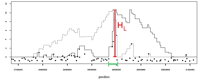
Let’s assume that we observe data at $L$ consecutive positions along a sequence, and that we have chosen a score function that transforms data at position $\ell$ into a real number $X_{\ell}$ . Here, we chose $X_{\ell}=-log10(p-value_{\ell})-\xi$ , where $p-value_{\ell}$ is the $p$ -value of a test at position $\ell$ and $\xi$ is an arbitrarily chosen real number. Then $X=(X_{1},\dots,X_{\ell},\dots,X_{L})$ is the resulting sequence of scores. We consider each chromosome as a sequence and $\ell$ refers to a fixed position on the chromosome (for instance a SNP). We further introduce the Lindley process $h=(h_{1},\dots,h_{\ell},\dots,h_{L})$ , with $h_{\ell}=max(0,h_{\ell-1}+X_{\ell})$ and $h_{0}=0$ .

The local score of the sequence $X$ is defined as:

H_{L}(X)=\max\limits_{1\leq\ell\leq L}h_{\ell}.

(1)

An equivalent way to apprehend the local score is to compute the maximum of the partial sums of the scores at adjacent loci: $H_{L}(X)=\max\limits_{1\leq i\leq j\leq L}\{X_{i}+X_{i+1}\dots+X_{j}\}$ .

The local score has an associated interval of interest $[\ell_{start}(X),\ell_{stop}(X)]$ enriched in high values of $X$ . The end of the interval is the locus where the local score is realized, i.e. $\ell_{stop}(X)=argmax_{\ell}\ h_{\ell}$ . The interval begins on the last locus before $\ell_{stop}(X)$ where the Lindley process is equal to 0, i.e. $\ell_{start}(X)=\max\{\ell\leq\ell_{stop},h_{\ell}=0\}$ .

The interval of interest is unchanged if we read the sequence in the opposite direction: denoting $\bar{X}=(X_{L},\dots,X_{\ell},\dots,X_{1})$ (i.e. $X_{i}=\bar{X}_{L-i+1}$ ), it can be shown that $\ell_{start}(X)=\ell_{stop}(\bar{X})$ and $\ell_{stop}(X)=\ell_{start}(\bar{X})$ , so the interval realizing the local score is easily highlighted. The notions of Lindley process, local score and the associated interval are illustrated in Figure 1.

The expectation $E(X)$ of the score should be negative to ensure the Lindley process to vanish at least once, in order to focus on local, instead of global, interest. Assuming that $p-value_{\ell}$ follows a uniform distribution, then $E(X)=\frac{1}{log(10)}-\xi$ , so $\xi$ should be approximately greater than $0.43$ . On the other hand, at least one score should be positive ( $\max\limits_{\ell}X_{\ell}>0$ ), which implies that $\xi<-log10(\min\limits_{\ell}(p-value_{\ell}))$ . In practice, it is up to the user to choose a value between $\frac{1}{L}\sum\limits_{\ell}-log10(p-value_{\ell})$ (close to 0.43 if the $p$ -values are approximately uniform under the null), and $-log10(\min\limits_{\ell}(p-value_{\ell}))$ . The greater $\xi$ , the closer we are to the single marker approach, since only the top markers will contribute to the Lindley process. The lower $\xi$ , the more often local maxima will appear in the Lindley process, and the larger will be the detected region.

Distribution of the local score under the null hypothesis

For independent sites (i.i.d. model) and integer scores it is possible to obtain exact $p$ -values for short sequences and approximate $p$ -values for long sequences (Karlin and Altschul, 1990, Karlin and Dembo, 1992, Mercier et al., 2003). Exact $p$ -values can be obtained in Markovian cases (Hassenforder and Mercier, 2007) but with a large computational time for such sequence length.

Real data however hardly meets the independence assumption. In quail data, the correlation of score function values of adjacent sites ranged from 0.22 to 0.47 for the 28 quail chromosomes, with a vast majority around 0.3. The maximum value (0.47) was reached for the ”shortest” chromosome, GGA16, which encountered alignment problems and was thus not included in further analyzes.

For a non zero correlation between sites, we propose to obtain approximate $p$ -values for the local score $H_{L}$ on a chromosome of length $L$ , assuming a constant auto-correlation along the genome. A first possibility is to compute an empirical distribution of the local score $H_{L}$ under the null hypothesis of neutrality, by way of simulations involving a given auto-correlation $\rho$ for the score function. This was achievable in quail just for short chromosomes (i.e. GGA28, 40,000 bp long), but the computational time was prohibitive for the largest ones (i.e. GGA1, 2,631,000 bp long).

Another possibility is to follow ideas of Guedj et al. (2006) and Robelin (2005), and to approximate the distribution of the local score with a Gumbel distribution, which in general is used to model maxima of stochastic processes. As the cumulative density function of a Gumbel variable is linear after a log(-log) transformation, for given values of the sequence length $L$ and the correlation $\rho$ , an empirical cumulative density function (ecdf) $F_{L,\rho}$ can be obtained by simulating sequences with these properties and fitting a linear model of the form

log(-log(F_{L,\rho}(y))=a_{L,\rho}+b_{L,\rho}y+e,

(2)

with $e\sim{\cal N}(0,\sigma_{L,\rho}^{2})$ , which provides estimates $\hat{a}_{L,\rho}$ and $\hat{b}_{L,\rho}$ of the parameters $a_{L,\rho}$ and $b_{L,\rho}$ (see Figure S2).

We applied this strategy for several values of $L$ (from 100 to 45000) and $\rho$ (from 0 to 0.9) (Figure S2). For each pair $(L,\rho)$ 5000 sequences $z_{i=1,...,L}$ were generated from a multivariate uniform distribution with autocorrelation $\rho$ , mimicking the null distribution of $p$ -values of single marker tests. Details of these simulations are given in Supporting Information, Section: Null distribution of the local score for correlated markers.

For a given value of $\xi$ , abacuses of parameters $\hat{a}_{L,\rho}-log(L)$ and $\hat{b}_{L,\rho}$ converge rapidely to a limit distribution from approximately $L=10{,}000$ (Figure S3). Thus, if the $p$ -values follow a uniform distribution, for sufficiently long sequences $a-log(L)$ and $b$ depend only of $\rho$ and are independent from $L$ . Taking advantage of this property, we further implemented a cubic and a quadratic fit that provide general approximations $\tilde{\hat{a}}_{L,\rho}$ and $\tilde{\hat{b}}_{L,rho}$ of $\hat{a}_{L,\rho}$ and $\hat{b}_{L,\rho}$ for any value of $L$ and $\rho$ (not only those simulated). These formulas can be found in Supporting Information, for $\xi=1$ and 2, and a script is given to compute the polynomes for other values of $\xi$ . The $p$ -value for the local score of any chromosome can be computed by first obtaining $a$ and $b$ from those formulas and then using equation (2), that is:

P(H_{L}\leq x)\approx 1-\exp\left(-\exp(\tilde{\hat{a}}_{L,\rho}+\tilde{\hat{b}}_{L,\rho}x)\right)

(3)

Remark that this formula has the same form as Karlin’s approximation in the independent case ( $\rho=0$ ), see Supporting Information. Similarly, threshold values $t_{L,\rho;\alpha}$ at $\alpha$ level for the local score can be obtained by

t_{L,\rho;\alpha}\approx\frac{log(-log(1-\alpha))-\tilde{\hat{a}}_{L,\rho}}{\tilde{\hat{b}}_{L,\rho}}.

(4)

This strategy was applied for the analysis of the sheep data, and could more generally be used by any future study for which the $p$ -values of single marker tests are uniformly distributed under the null hypothesis.

However, as described in the Data Section (2.1) the quail data has many particularities. One of them is a particularly strong genetic drift, resulting in a very high frequency of fixed alleles. This implies that the neutral distribution of $\mathcal{F}$ -LK is no longer a chi-square, in contrast to what is assumed when computing the $p$ -values of this test. Consequently, the $p$ -value distribution of $\mathcal{F}$ -LK under the null hypothesis is not uniform and the strategy described above cannot be applied in this particular case.

To get an approximate null distribution for the local scores obtained from the quail data, we thus used a slightly different strategy, based on the re-sampling of score sequences of fixed length from the quail data (see the Supporting Information for more details, Figures S4-S6, Tables S1-S2). This provided estimates $\tilde{\hat{a}}_{L,\rho}$ and $\tilde{\hat{b}}_{L,\rho}$ of $\hat{a}_{L,\rho}$ and $\hat{b}_{L,\rho}$ , and hence of $a_{L,\rho}$ and $b_{L,\rho}$ :

	$\displaystyle\hat{a}_{L,\rho}=log(L)-7.60-6.86\rho$		(5)
	$\displaystyle\hat{b}_{L,\rho}=-0.49+1.51\rho$		(6)

which are only valid locally around $\rho=0.3$ , and are thus applicable to all quail chromosomes except GGA16 (whose auto-correlation is 0.47).

3 Results

3.1 Benchmark 1: Lactase region of HapMap data

We tested a 4Mb region (134-138 Mb) on Human chromosome 2 containing the LCT gene, because a known causal mutation for the lactase persistent phenotype in the CEU (Utah Residents with Northern and Western European ancestry) population is located in chromosome 2 at position 136,325,116. Data was taken from the HapMap Phase III dataset and consisted in the genotypes of 370 founder individuals from the CEU, TSI (Toscani in Italy), CHB (Han Chinese in Bejing, China) and JPT (Japanese in Tokyo, Japan) populations. Only $25\%$ of the available SNPs (that is 497 SNPs) were included in the analysis.

We compared results obtained from the single locus approach $\mathcal{F}$ -LK (Bonhomme et al., 2010), the local score and the haplotypic approach hapFLK (Fariello et al., 2013) (Figure 2). While the top markers for $\mathcal{F}$ -LK were quite far from the Lactase gene, The intervals given by hapFLK and the local score were really close to the Lactase gene, with the local score providing a smaller interval. Here, the local score was based on the score function $-log10(p-value_{\mathcal{F}-LK})-1$ , meaning that $p$ -values of single marker tests greater than $10^{-1}$ were cumulated to find an interval achieving the local score. On this benchmark region, the local score clearly highlighted a well known target of selection in Human, thus performing as well as the hapFLK test.

3.2 Benchmark 2: Sheep HapMap data

The Sheep HapMap dataset includes individual genotypes at 60K SNPs for 2819 animals from 74 worldwide sheep breeds (Kijas et al., 2012). A genome scan for selection was performed on this dataset using single marker $F_{ST}\$ (Kijas et al., 2012). We considered here a subset of this dataset: a group of 4 breeds (two Spanish breeds and two French breeds) originating from South-western Europe (256 sheep). Genome scans for selection using the single marker test $\mathcal{F}$ -LK and the haplotypic test hapFLK have already been performed in this group (Fariello et al., 2014). Interestingly, genome scans with $\mathcal{F}$ -LK and hapFLK lead to distinct detected regions.

Here, the score was $X_{\ell}=-log10(p-value_{\mathcal{F}-LK})-\xi$ , with $\xi=1$ or 2 (Figure S7). The approaches taking account of the dependence between adjacent markers (the local score and hapFLK) gave a clear picture of different selection signatures. Using the single SNP test $\mathcal{F}$ -LK, with a false discovery rate of 5%, none of SNPs reached the significance threshold.

The local score approach highlighted a region on OAR10 (either for $\xi=1$ or 2) that was not significant either for $\mathcal{F}$ -LK or for hapFLK (Figure 1). In this region, no particular haplotype was selected, but a few SNPs whose alleles were shared in several haplotypic backgrounds showed a moderate signal. This region is very close to RXFP2 for which polymorphisms have been shown to affect horn size and polledness in the Soay (Johnston et al., 2010) and Australian Merino (Dominik et al., 2012).

The CPU time for a whole genome scan with hapFLK was about a few hours, while it took only a few minutes to compute $\mathcal{F}$ -LK and a few more minutes to compute the local score. The significance threshold for each chromosome was computed using Equations (S9) and (S11) in Supporting information. This computation time does not include the simulations that were used to obtain the $p$ -values, because these simulations had to be performed only once and the formulas we obtained can now be used directly, if the $p$ -values follow a uniform distribution.

3.3 Quail data

We looked for genome wide selection signatures in two divergent Quail lines. We used the local score associated to the score function $-log10(p-value_{F_{ST}})-1$ , ( $F_{ST}$ and $\mathcal{F}$ -LK are equivalent here).

We first focused on GGA1 and compared the local score approach with several sliding window statistics (Figure 3): (i) the mean $F_{ST}$ , (ii) the proportion of ”significant” SNPs, i.e. such that $-log10(p-value_{F_{ST}})$ is greater than 1, and (iii) the proportion of differentially fixed SNPs, i.e. that have reached fixation in one line and were lost in the other one. These statistics were computed over windows of 10kb, which included 132 SNPs on average. We used the top $1\%$ of the distribution of the statistic genome wide as significance threshold for this windowed statistics. All statistics had a local maximum in the same region as the Lindley process, indicating that in this particular region there is an excess of differentially fixed SNPs. On the other hand, the large number of local maxima exceeding the threshold for these statistics, suggests that many of them may be false positives. A second peak, at position roughly 150000, was observed with almost all statistics but not with the local score.

The region detected by the local score on GGA1 was 219.23 kb long and contained 2646 SNPs. The SNP density in this region was 74.8 SNPs per 10kb. It is less than the whole genome average, suggesting that this region is probably not a false positive due to a greater density of SNPs. In addition, the autocorrelation in this region was not an outlier, compared to the autocorrelations of windows of the same size in the same chromosome (Figure 4). The region displayed a slightly decreased average $\mathcal{F}$ -LK p-value, and a slightly larger proportion of ”significant” SNPs or fixed SNPs per window (Figure 3), but this did not appear very clearly on the graphs, in contrast with the local score signal.

The local score (maximum value of the Lindley process) was in the range 11-50 for almost all chromosomes, except chromosomes GGA1 (with a local score equal to 279.73), GGA2 (local score 150.78), GGA3 (local score 184.25) and GGA6 (local score 286.43) (Table S3, Figure S10). A very clear peak was observed in these cases, in contrast with windowed $F_{ST}$ (Figures 3, S8 and S9).

Detected regions, mapped on the chicken genomic sequence, are listed in Table 1. Local score profiles and the $5\%$ and $1\%$ rejection thresholds are included in the Supplementary Information. Detected regions were in general very short (from 19 to 219kb) and included at most 3 genes. This accurate detection of the region under selection is a clear advantage for understanding the selective process that has been acting in these lines, and holds great promises for the identification of the exact polymorphisms under selection, which could be the aim of subsequent studies. The two regions of chromosome 4 do not reach the $5\%$ threshold, but we decided to include them because they contain interesting candidate genes (see Discussion).

4 Discussion

The work presented here showed a clear added value of a statistical method and a data set. The methodology developed was the only one to provide a short list of candidate genes related to the selected behavioral trait in the quail lines.

Candidate genes

Several genes comprised or partially localized in the detected regions under selection in Quail, have been associated with autistic disorders (http://genome.ucsc.edu/cgi-bin/hgTracks). PTPRE (receptor-type tyrosine-protein phosphatase epsilon precursor, in region 7) is one of the candidate genes present on human chromosome 10q26 and has been shown to be involved in autism spectrum disorder (Tonk VS, 2011). Similarly, ARL13B (in region 1) is one of the genes involved in the Joubert syndrome (Cantagrel et al., 2008), a psychiatric disorder with possible autistic symptoms (Doherty, 2009). Finally, IMPK (inositol polyphosphate multikinase, in region 8) maps to a position homologous to a region of human chromosome 10 (10q21.1) which shows a male-only signal of linkage with a social responsiveness trait (Duvall et al., 2007). This study detected social responsiveness quantitative trait loci in multiplex autism families. As the linkage region in human is quite large, more work has to be done before considering this gene as a functional candidate.

Autistic spectrum disorders are observed in a number of disorders that have very different etiology, including fragile X Syndrome, Rett Syndrome or Foetal Anticonvulsant Syndrome. While these disorders have very different underlying etiologies, they share common qualitative behavioral abnormalities in domains particularly relevant for social behaviors such as language, communication and social interaction (Rutter, 1978, Association, 2000). In line with this, a number of experiments conducted on High Social Reinstatement (HSR) and Low Social Reinstatement (LSR) quails indicate that the selection program carried out with these lines is not limited to selection on a single response, social reinstatement, but affect more generally the ability of the quail to process social information. Differences in social motivation, but also individual recognition have been described between LSR and HSR quail (François et al., 2000b, Schweitzer et al., 2010). Inter-individual distances are longer in LSR quail (François et al., 2000b) and LSR young quails have decreased interest in unfamiliar birds (François et al., 2000a) and lower isolation distress than HSR ones (see Jones and Mills (1999) for review). A last interesting candidate gene is CTNNA2 (catenin alpha 2, in region 6). This gene, involved in synaptic plasticity, has been shown to be implicated in several behavioral traits, and has recently been associated with excitement-seeking, partly related to social behavior (Terracciano et al., 2011). These genes may thus represent particularly relevant candidates to explain the difference between two quail lines that diverge on many aspects of social behavior. Further experiments will be required to examine the possible functional link between the selected genes and the divergent phenotype observed in these lines.

Generality of the local score

We proposed a new method to detect selection signatures genome-wide, which takes linkage disequilibrium into account even when individual genetic information is not available. The strategy is to use the local score theory (which is widely used in sequence alignment, for example) to cumulate information of single marker significance over the genome, in order to detect intervals of high cumulated significance.

This strategy only requires a significance or importance value (the score) for each marker. Here we focused on the detection of regions with outstanding genetic differentiation between populations and proposed to build the score from the $p$ -value of a single marker test (e.g. $F_{ST}$ or $\mathcal{F}$ -LK). Thus, the distribution of the local score only depends on the distribution of single marker test $p$ -values, which, under the null hypothesis, can generally be assumed to be uniform. This approach gave a clear picture of the selection targets in 2 benchmark data sets (the human HapMap and the SheepHapMap) including individual genotypic information obtained from SNP chips. In SheepHapMap data we detected signals that were not detected by hapFLK (e.g. the horn SNPs). We also failed to recover some of the signals detected by hapFLK, but this may be related to the low SNP density of this data set. Indeed, as the local score approach is based on the concentration of SNPs with low $p$ -values, even strong selection events might be difficult to detect if only few SNPs are found in the region.

With high density data, the local score might thus detect a wide range of signals, from moderate signals spanning over a large region to strong but short signals. The former class of signals could typically arise from recent selection events where the selected haplotype did not yet fix in the population (this is the case for the human Lactase signal), as well as from recent soft sweeps, i.e. where the selected allele is associated to several haplotype backgrounds. In contrast, the latter class of signals would correspond to old hard sweep signals, whose length has already been reduced by recombination. This is for instance the case of the horn locus in sheep.

Choosing $\xi$

Among other factors, the type of selection events that are detected with the local score approach depends on the choice of $\xi$ , the threshold below which small $p$ -values are cumulated. This value must be included between 0.43 and $-log10(\min\limits_{\ell}(p-value_{\ell}))$ , with high values leading to focus on the few strongest SNPs and low values allowing to cumulate a larger number of intermediate signals. In the quail data, the large amount of drift implies that the best single marker $p$ -value (corresponding to an allele frequency of 0 in one line and 1 in the other) was $10^{-1.5}$ , so the upper bound for $\xi$ was 1.5. In this case, cumulating $p$ -values under $10^{-1}$ appeared appropriate, since it allowed to cumulate a large number of signals, while excluding $p$ -values above $10^{-1}$ that can hardly be considered as significant. Besides, due to the short evolution time since the divergence of the two lines (and consequently the advent of the selective constraint in each of them), we expected to detect recent soft or incomplete sweeps rather than old hard sweeps, which again argues for the use of a low value of $\xi$ .

In the sheep data (Figure S7), the use of two different values of $\xi$ seemed to lead to two different detection patterns: for $\xi=1$ the data showed more local maxima than for $\xi=2$ . But, when thresholds were computed, we observed that the significant local maxima were almost the same for $\xi=1$ and $\xi=2$ .

Computing $p$ -values of the local score

Assuming that the values of the scores are independent, formulas for computing the $p$ -values of the global maximum of the Lindley process have been proposed in different scenarios (the main difference was the length of the sequence and the computation of approximations or exact $p$ -values) (Karlin and Altschul, 1990, Karlin and Dembo, 1992, Mercier and Daudin, 2001, Mercier et al., 2003). Since then, local score procedures have been used, for example for aligning sequences, and the independence assumption was always used for computing the $p$ -values, even if it was clearly wrong. This shows how difficult it is to take dependence into account. Following ideas of (Robelin, 2005) we proposed to find the empirical distribution of the local score, as a function of $\rho$ and $L$ , for a particular $\xi$ . From simulations, we learned how the parameters $a-log(L)$ and $b$ depend from $\rho$ (for a fixed $\xi$ ), given that the distribution of the $p$ -values of single marker tests is uniform. The polynomes given in Supporting Information can now be used to compute parameters $a$ and $b$ of the Gumbel distribution in future studies, (even related to a totally different question), as long as single marker $p$ -values are uniformly distributed under the null distribution, and $\xi=1$ or 2.

If the $p$ -values do not follow a Gumbel distribution, a re-sampling strategy, similar to the one implemented for the Quail data, will be necessary. In the quail data, this strategy could be implemented because we observed from simulations that the parameters $a-log(L)$ and $b$ converged to a limit for not too large values of $L$ . This allowed to estimate parameters of long sequences using simulations from shorter sequences. In the future, further investigations should however be carried out to find a better and more general way of estimating the $p$ -values.

Our method supposes a constant auto-correlation along the each chromosome. Even if we know that this is not true, this provided at least a way to take marker dependencies into account. Further research is also needed in order to consider changes of LD along the chromosome, which would likely require a modification of the score function.

Pros and cons of competing detection methods in presence of high drift

The quail experiment perfectly illustrates the difficulty to distinguish selective processes from neutral processes, and the importance to cumulate signals from multiple markers to overcome it. Indeed, a lot of drift has been cumulated in the two quail lines, because only 60 individuals were kept at each generation, so that markers with high $F_{ST}$ values are very likely even under the null hypothesis of neutrality. For instance, $1.5\%$ of the markers on GGA1 were fixed differentially in the two lines and thus achieved the maximal $F_{ST}$ value. A large proportion of these differential fixations might be just due to drift. Consequently, considering all markers in the top $1\%$ of the $F_{ST}$ distribution as selection candidates, which is a common practice in single marker based genome scans, must result here in a large proportion of false positives.

As selection does not only raise up the frequency of the selected allele, but also of other alleles in its neighborhood, we expect to find an increased amount of markers with high $F_{ST}$ value around a selected mutation. Johansson et al. (2010) exploited this property by looking for clusters of alleles that were fixed for alternative alleles in the divergent lines. Because of linkage disequilibrium, we expect that some of the alleles in the neighborhood of the selected variant will be fixed differentially in the two lines. However, in this type of experiments, selection generally does not act on new variants (divergence time is probably too small for new advantageous mutations to appear) but on variants that were already segregating in the founder population. So, at many other sites we just expect an increased allele frequency difference between the two lines, but not necessarily differential fixation. Consequently, alleles showing a large difference in allele frequencies between the two lines are also informative, even though a bit less than differentially fixed ones.

The local score approach tries to take advantage of this information, as alleles that are not fixed but have a high $F_{ST}$ value also contribute to the local score. Actually, the local score proposed here can be seen as a generalization of the clustering method of Johansson et al. (2010), where the markers would get a positive score if they are differentially fixed, and a negative or zero score otherwise. When analyzing the quail data, we tried a windowing approach based on the number of differentially fixed SNPs in each window. Although our definition of fixed SNPs was a bit more liberal than that of (Johansson et al., 2010) (the allele had to be fixed in only one line), this approach was quite similar in spirit. No clear signal could be detected with this approach, in contrast to the local score, confirming the fact that cumulating information from all allele frequency differences is very important.

Another interest of cumulating signals from consecutive markers, as implemented in the local score, is to reduce the noise arising from sequencing errors. Such errors are unavoidable with next bio-technologies in general, and with next generation sequencing in particular. They result in a lower accuracy when estimating allele frequencies at a SNP, which is even decreased in the case of pooled samples with small sample size. In the quail experiment, pools of only 10 diploid individuals were used. But, using a method specifically designed to improve the estimation of allele frequencies from pooled samples (Boitard et al., 2013) (see also (Ferreti et al., 2013) who showed that individual and pooled estimates can be highly correlated), and cumulating single marker signals using the local score, we could extract rich information from this relatively small sample size.

Looking for information from founder population

Sequencing the founder population of the two quail lines would increase our power to detect selection and improve our understanding of the selective process in a given region (Laval et al., 2003). Indeed, sequencing the ancestral population provides a precise estimation of founder allele frequencies. Without this information, founder allele frequencies are estimated by the mean of the allele frequencies in the two divergent lines. This estimation procedure is the best we can imagine in this situation, but it is clearly biased for sites under selection. Imagine for instance that an allele with initial frequency 0.1 increases in frequency in line 1 due to selection, and is lost in line 2 due to drift. The allele frequency trajectory in line 1 clearly suggests the influence of positive selection. But from the final allele frequencies (0 and 1) we will assume that founder allele frequency was 0.5, so that allele frequency trajectories in the two populations are less informative. Similarly, the identification of the SNPs and the population with the highest allele frequency variation would be much more accurate if ancestral allele frequencies were known.

For future similar studies, we therefore recommend to also sequence individuals from the founder population or, if not possible, to sequence a higher number of present populations in order to better estimate ancestral allele frequencies (see the discussion in (Bonhomme et al., 2010, Fariello et al., 2013)).

5 Conclusion

This work enhanced the added value of a divergent selection experiment on a behavior trait, pool sequencing of two divergent lines, and an appropriate statistical approach: here the local score. All this combined lead to the discovery of eight small genomic regions exhibiting candidate genes related to autism and social behavior.

Besides, other studies, like Genome Wide Association Studies (GWAS), could also gain in applying this local score strategy, as proposed by Guedj et al. (2006), Robelin (2005), Teyssedre et al. (2012), in particular when $p$ -values are not extreme and when marker density is high (as in the experiment of Johansson et al. (2010)). In genome scans for selection, the local score approach can be applied to data with or without individual genotypic information and any statistic.

6 Supplementary Material

Supplementary tables S1-S7 and figures S1-S11 are available at

7 Acknowledgments

This work was supported by the French Agence Nationale de la Recherche provided to C.L. (SNP-BB project, ANR-009-GENM-008) for the sequencing, and to M.S.C. and S.B. (DéLiSus project, ANR-07-GANI-001) for the methodology. The Région Midi-Pyrénées, the Département de Génétique Animale of Institut National de la Recherche Agronomique and Agencia Nacional de Investigación e Innovación provided financial support for the salary of M.I.F. Sequencing was performed at GeT-PlaGe Genotoul platform. Data analyses were performed on the computer cluster of the bioinformatics platform Toulouse Midi-Pyrénées. We thank Bertrand Servin for stimulating discussions.

References

Association (2000) American Psychiatric Association. Diagnostic and statistical manual of mental disorders: DSM IV. American Psychiatric Association, 2000.
Bhatia et al. (2011) G. Bhatia, N. Patterson, B. Pasaniuc, N. Zaitlen, G. Genovese, S. Pollack, S. Mallick, S. Myers, A. Tandon, C. Spencer, C. D. Palmer, A. A. Adeyemo, E. L. Akylbekova, L. A. Cupples, J. Divers, M. Fornage, W. H. Kao, L. Lange, M. Li, S. Musani, J. C. Mychaleckyj, A. Ogunniyi, G. Papanicolaou, C. N. Rotimi, J. I. Rotter, I. Ruczinski, B. Salako, D. S. Siscovick, B. O. Tayo, Q. Yang, S. McCarroll, P. Sabeti, G. Lettre, P. De Jager, J. Hirschhorn, X. Zhu, R. Cooper, D. Reich, J. G. Wilson, and A. L. Price. Genome-wide comparison of African-ancestry populations from CARe and other cohorts reveals signals of natural selection. Am. J. Hum. Genet., 89(3):368–381, Sep 2011.
Boitard et al. (2009) S. Boitard, C. Schloetterer, and A. Futschik. Detecting selective sweeps: a new approach based on hidden markov models. Genetics, 181:1567–1578, 2009.
Boitard et al. (2013) S. Boitard, R. Kofler, P. Francoise, D. Robelin, C. Schlotterer, and A. Futschik. Pool-hmm: a Python program for estimating the allele frequency spectrum and detecting selective sweeps from next generation sequencing of pooled samples. Mol Ecol Resour, 13(2):337–340, Mar 2013.
Bonhomme et al. (2010) M. Bonhomme, C. Chevalet, B. Servin, S. Boitard, J. Abdallah, S. Blott, and M. San Cristobal. Detecting selection in population trees: The Lewontin and Krakauer test extended. Genetics, 186(1):241–262, 2010.
Cantagrel et al. (2008) V. Cantagrel, J. L. Silhavy, S. L. Bielas, D. Swistun, S. E. Marsh, J. Y. Bertrand, S. Audollent, T. Attie-Bitach, K. R. Holden, W. B. Dobyns, D. Traver, L. Al-Gazali, B. R. Ali, T. H. Lindner, T. Caspary, E. A. Otto, F. Hildebrandt, I. A. Glass, C. V. Logan, C. A. Johnson, C. Bennett, F. Brancati, E. M. Valente, C. G. Woods, and J. G. Gleeson. Mutations in the cilia gene ARL13B lead to the classical form of Joubert syndrome. Am. J. Hum. Genet., 83(2):170–179, Aug 2008.
Chen et al. (2010) H. Chen, N. Patterson, and D. Reich. Population differentiation as a test for selective sweeps. Genome Res., 20(3):393–402, Mar 2010.
Doherty (2009) D. Doherty. Joubert syndrome: insights into brain development, cilium biology, and complex disease. Semin Pediatr Neurol, 16(3):143–154, 2009.
Dominik et al. (2012) S. Dominik, J. M. Henshall, and B. J. Hayes. A single nucleotide polymorphism on chromosome 10 is highly predictive for the polled phenotype in Australian Merino sheep. Anim Genet, 43(4):468–70, 2012. URL http://eutils.ncbi.nlm.nih.gov/entrez/eutils/elink.fcgi?cmd=prlinks&dbfrom=pubmed&retmode=ref&id=22497244.
Duvall et al. (2007) J. A. Duvall, A. Lu, R. M. Cantor, R. D. Todd, J. N. Constantino, and D. H. Geschwind. A quantitative trait locus analysis of social responsiveness in multiplex autism families. Am J Psychiatry, 164(4):656–662, Apr 2007.
Fariello et al. (2013) M. I. Fariello, S. Boitard, H. Naya, M. SanCristobal, and B. Servin. Detecting signatures of selection through haplotype differentiation among hierarchically structured populations. Genetics, 193(3):929–941, Mar 2013.
Fariello et al. (2014) Maria-Ines Fariello, Bertrand Servin, Gwenola Tosser-Klopp, Rachel Rupp, Carole Moreno, Magali San Cristobal, Simon Boitard, and International Sheep Genomics Consortium. Selection signatures in worldwide sheep populations. PLoS ONE, 9(8):e103813, 08 2014. doi: 10.1371/journal.pone.0103813. URL http://dx.doi.org/10.1371%2Fjournal.pone.0103813.
Ferreti et al. (2013) L. Ferreti, Ramos-Onsins S.E., and M. Perez-Enciso. Population genomics from pool sequencing. Mol. Ecol., 22:5561–76, 2013.
François et al. (2000a) N. François, S. Decros, and et al. Effect of group disruption on social behaviour in lines of Japanese quail (Coturnix japonica) selected for high or low levels of social reinstatement behaviour. Behavioural Processes, 48(3):171–181, 2000a.
François et al. (2000b) N. François, A. D. Mills, and et al. Inter-individual distances during open-field tests in Japanese quail (Coturnix japonica) selected for high or low levels of social reinstatement behaviour. Behavioural Processes, 47(2):73–80, 2000b.
Guedj et al. (2006) M. Guedj, D. Robelin, M. Hoebeke, M. Lamarine, J. Wojcik, and G. Nuel. Detecting local high-scoring segments: a first-stage approach for genome-wide association studies. Stat Appl Genet Mol Biol, 5:Article22, 2006.
Hassenforder and Mercier (2007) C. Hassenforder and S. Mercier. Exact distribution of the local score for Markovian sequences. Annals of the Institute of Statistical Mathematics, 59(4):741–55, 2007.
Johansson et al. (2010) A. M. Johansson, M. E. Pettersson, P. B. Siegel, and O. Carlborg. Genome-wide effects of long-term divergent selection. PLoS Genet., 6(11):e1001188, Nov 2010.
Johnston et al. (2010) S.E. Johnston, D. Beraldi, A.F. McRae, J.M. Pemberton, and J. Slate. Horn type and horn length genes map to the same chromosomal region in Soay sheep. Heredity, 104:196–205, 2010.
Jones and Mills (1999) R.B. Jones and A.D. Mills. Divergent selection for social reinstatement behaviour in Japanese quail: Effects on sociality and social discrimination. Poultry and Avian Biology Reviews, 10:213–223, 1999.
Karlin and Altschul (1990) S. Karlin and S.-F. Altschul. Methods for assessing the statistical significance of molecular sequence features by using general scoring schemes. PNAS, 87:2264–2268, 1990.
Karlin and Dembo (1992) S. Karlin and A. Dembo. Limit distributions of maximal segmental score among Markov-dependent partial sums. AdAP, 24:113–140, 1992.
Kijas et al. (2012) James W. Kijas, Johannes A. Lenstra, Ben Hayes, Simon Boitard, Laercio R. Porto Neto, Magali San Cristobal, Bertrand Servin, Russell McCulloch, Vicki Whan, Kimberly Gietzen, Samuel Paiva, William Barendse, Elena Ciani, Herman Raadsma, John McEwan, Brian Dalrymple, and other members of the International Sheep Genomics Consortium. Genome-wide analysis of the world’s sheep breeds reveals high levels of historic mixture and strong recent selection. PLoS Biol, 10(2):e1001258, 02 2012. doi: 10.1371/journal.pbio.1001258. URL http://dx.doi.org/10.1371%2Fjournal.pbio.1001258.
Laval et al. (2003) G. Laval, M. San Cristobal, and C. Chevalet. Maximum-likelihood and markov chain monte carlo approaches to estimate inbreeding and effective size from allele frequency changes. Genetics, 164:1189–1204, 2003.
Li and Durbin (2009) H. Li and R. Durbin. Fast and accurate short read alignment with burrows-wheeler transform. Bioinformatics, 25:1754–60, 2009.
Mercier and Daudin (2001) S. Mercier and J. J. Daudin. Exact distribution for the local score of one i.i.d. random sequence. J. Comput. Biol., 8(4):373–380, 2001.
Mercier et al. (2003) S. Mercier, D. Cellier, and D. Charlot. An improved approximation for assessing the statistical significance of molecular sequence features. Applied Probability Trust, 2003.
Mills and Faure (1991) A.D. Mills and J.M. Faure. Divergent selection for duration of tonic immobility and social reinstatement behavior in Japanese Quail (Coturnix coturnix japonica) chicks. Journal of Comparative Psychology, 105:25–38, 1991.
Myles et al. (2008) S. Myles, K. Tang, M. Somel, R. E. Green, J. Kelso, and M. Stoneking. Identification and analysis of genomic regions with large between-population differentiation in humans. Ann. Hum. Genet., 72:99–110, Jan 2008.
Nielsen et al. (2005) R. Nielsen, L. Williamson, Y. Kim, M.J. Hubisz, A.G. Clark, and C. Bustamante. Genomic scans for selective sweeps using SNP data. Genome Research, 15:1566–1575, 2005.
Pritchard et al. (2010) J. K. Pritchard, J. K. Pickrell, and G. Coop. The genetics of human adaptation: hard sweeps, soft sweeps, and polygenic adaptation. Curr. Biol., 20(4):R208–215, Feb 2010.
Qanbari et al. (2012) S. Qanbari, T.M. Strom, G. Haberer, S. Weigend, A.A. Gheyas, F. Turner, D.W. Burt, R. Preisinger, D. Gianola, and H. Simianer. A high resolution genome-wide scan for significant selective sweeps: An application to pooled sequence data in laying chickens. PLOS One, 7(1):e49525, 2012. URL http://www.plosone.org/article/fetchObject.action?uri=info%3Adoi%2F10.1371%2Fjournal.pone.0049525&representation=PDF.
Richard et al. (2008) S. Richard, C. Arnould, D. Guemene, C. Leterrier, S. Mignon-Grasteau, and et al. Emotional reactivity in the quail: an integrated approach to animal welfare. INRA Productions Animales, 21:71–77, 2008.
Robelin (2005) D. Robelin. Détection de courts segments inversés dans les génomes : méthodes et applications. PhD thesis, Université Paris XI, 2005.
Roussot et al. (2003) O. Roussot, K. Feve, and et al. AFLP linkage map of the Japanese quail Coturnix japonica. Genet Sel Evol, 35(5):559–572, 2003.
Rutter (1978) M. Rutter. Diagnosis and definition of childhood autism. J Autism Child Schizophr, 8(2):139–161, 1978.
Sabeti et al. (2002) Pardis C. Sabeti, David E. Reich, John M. Higgins, Haninah Z. P. Levine, Daniel J. Richter, Stephen F. Schaffner, Stacey B. Gabriel, Jill V. Platko, Nick J. Patterson, Gavin J. McDonald, Hans C. Ackerman, Sarah J. Campbell, David Altshuler, Richard Cooper, Dominic Kwiatkowski, Ryk Ward, and Eric S. Lander. Detecting recent positive selection in the human genome from haplotype structure. Nature, 419:832–837, 2002.
Sabeti et al. (2007) Pardis C. Sabeti, Patrick Varilly, Ben Fry, Jason Lohmueller, Elizabeth Hostetter, Chris Cotsapas, Xiaohui Xie, Elizabeth H. Byrne, Steven A. McCarroll, Rachelle Gaudet, Stephen F. Schaffner, and Eric S. Lander. Genome-wide detection and characterization of positive selection in human populations. Nature, 449:913–918, 2007.
Schweitzer et al. (2010) C. Schweitzer, C. Houdelier, S. Lumineau, F. Levy, and C. Arnould. Social motivation does not go hand in hand with social bonding between two familiar japanese quail chicks, coturnix japonica. Animal Behaviour, 79:571–578, 2010.
Schweitzer et al. (2011) C. Schweitzer, F. Levy, and C. Arnould. Increasing group size decreases social bonding in young japanese quail, coturnix japonica. Animal Behaviour, 81:535–542, 2011.
Terracciano et al. (2011) A. Terracciano, T. Esko, and et al. Meta-analysis of genome-wide association studies identifies common variants in ctnna2 associated with excitement-seeking. Transl Psychiatry, 1:e49, 2011.
Teyssedre et al. (2012) S. Teyssedre, M. C. Dupuis, G. Guerin, L. Schibler, J. M. Denoix, J. M. Elsen, and A. Ricard. Genome-wide association studies for osteochondrosis in French Trotter horses. J. Anim. Sci., 90(1):45–53, Jan 2012.
Tonk VS (2011) Wilson GN Tonk VS. Autism spectrum disorder with microdeletion 10q26 by subtelomere fish. Pediatric Health, Medicine and Therapeutics, 2:49–53, 2011. doi: http://dx.doi.org/10.2147/PHMT.S15665.
Voight et al. (2006) Benjamin F Voight, Sridhar Kudaravalli, Xiaoquan Wen, and Jonathan K Pritchard. A map of recent positive selection in the human genome. PLoS Biol, 4:e72, 2006.
Weir et al. (2005) B. S. Weir, L. R. Cardon, A. D. Anderson, D. M. Nielsen, and W. G. Hill. Measures of human population structure show heterogeneity among genomic regions. Genome Res, 15(11):1468–76, 2005. URL http://eutils.ncbi.nlm.nih.gov/entrez/eutils/elink.fcgi?cmd=prlinks&dbfrom=pubmed&retmode=ref&id=16251456.
Weir and Cockerham (1984) B.S. Weir and C.C. Cockerham. Estimating $f$ -statistics for the analysis of population structure. Evolution, 38:1358–1370, 1984.

Refer to caption — Figure 1: Example of local score on a chromosome segment in sheep: region related to the presence/absence of horns. Single marker significance is displayed by black points, representing $-log10(p-value_{\mathcal{F}-LK})-1$ for a $\mathcal{F}$ -LK test of neutrality. Three consecutive SNPs with high scores have been associated to the presence/absence of horns (Johnston et al., 2010). The Lindley process of the score function $-log10(p-value_{\mathcal{F}-LK})-1$ is drawn with a solid line going from the left to the right of the chromosome, and with a dashed line from the right to the left. The local score $H_{L}$ is achieved at the red arrow. The corresponding segment, materialized in green, contains exactly the 3 SNPs.

Figure 2: Selection footprints in human HapMap data: focus on Lactase region. (Top)

-log10(p-value_{\mathcal{F}-LK})

of the single marker

\mathcal{F}

-LK test. (Middle) Lindley process based on the score function

-log10(p-value_{\mathcal{F}-LK})-1

starting from the left (black) and from the right (red). Dotted vertical lines indicate the limits of the detected interval (achieving the local score). (Bottom) hapFLK values. Dotted vertical lines indicate the limits of the detected interval. The Lactase gene is located within the 2 vertical solid lines.

Reg.	GGA	Position	L (kb)	Gene name	Description
1	1	92,963,200-93,182,431	219	NSUN3	putative methyltransferase NSUN3
				ARL13B	ADP-ribosylation factor-like protein 13B
2	2	1,583,808-1,688,282	105	VIPR1	vasoactive intestinal polypeptide receptor
					1 precursor
3	3	61,585,151-61,604,462	19	ECHDC1	ethylmalonyl-CoA decarboxylase
				RNF146	ring finger protein 146
4	3	75,088,236-75,170,475	82	MMS22L	protein MMS22-like
5	4	11,412,108-11,452,505	40	GLOD5	Glyoxalase domain-containing protein 5
6	4	90,952,530-91,008,189	56	CTNNA2	catenin (cadherin-associated protein) $\alpha$ -2
7	6	35,234,541-35,336,717	102	FOXI2	forkhead box protein I3
				PTPRE	receptor-type tyrosine-protein phosphatase
					$\epsilon$ precursor
8	6	6,311,686-6,644,350	333	UBE2D1	ubiquitin-conjugating enzyme E2 D1
				CISD1	CDGSH iron sulfur dom-containing prot 1
				IPMK	inositol polyphosphate multikinase

Table 1: Footprints of selection in the quail experiment including two divergent lines for social behavior, and the genes included in each detected region (mapped on chicken genome).