Temperature Regulation in Multicore Processors Using Adjustable-Gain Integral Controllers

The end of Dennard scaling has led to increasing power densities on the processor die and consequently higher chip temperatures [1, 2]. Emerging and future processors are thermally limited and must operate within the cooling capacity of the chip package, which is typically represented by the maximum operating temperature. Dynamic Thermal Management (DTM) techniques have emerged to manage thermal behaviors and are challenged by a number of phenomena. In particular, the exponential dependence of static power on temperature limits the effectiveness of many existing DTM techniques. This coupling can also lead to thermal runaway that must be prevented by DTM to avoid damaging the chip. Furthermore, the structure of the thermal field matters as spatial and temporal variations in the thermal field degrade device reliability and accelerate chip failures. Similarly, rapid changes in the thermal field referred to as thermal cycling, also cause thermal stresses that degrade device and hence chip reliability.

A specific class of thermal regulation techniques includes activities’ management like instruction fetch throttling and clock gating  [3, 4], thread migration (computations’ rescheduling)  [5, 6], and core frequency scaling  [7]. References  [3, 4] use PI and PID controls to slow down the rate of the instruction-fetch unit whenever the temperature exceeds a given upper bound, while  [5, 6] schedule threads (computations) from hot cores to cooler cores in effort to maintain a balanced thermal field. Initial heuristic approaches started giving way to control-theoretic formalisms, with the aforementioned references  [3, 4] providing (to our knowledge) the earliest examples. Subsequently, Reference [8] considered a similar upper-bound regulation problem but uses Dynamic Voltage Frequency Scaling (DVFS) for temperature control. More recently [9] described a controller for regulating the fluid in a microfluidic heat sink based on the measured temperature as well as predicted temperature estimated from the projected power profile. Other work has investigated DTM under soft and hard real-time constraints [10, 11] seeking to satisfy thermal upper bounds while operating under scheduling constraints.

More recently, there emerged a number of approaches, which are based on optimal control and optimization. Reference [12] minimizes a least-square difference between the working frequency and the frequency mandated by the operating system, subject to thermal and frequency constraints, by using model-predictive control. Reference [13] uses similar techniques to minimize the least-square difference between set power levels and actual power levels in a core. Reference [14] uses a combination of off-line convex optimization and on-line control to obtain uniform spatial temperature gradient across several cores in a processor. We point out that these references assume linear and time-invariant plant-models for their respective control systems; [13] updates the model on-line while [12, 14] do not. Finally, reference [15] minimizes energy consumption while preserving performance levels within a tolerable limit by employing separate Model Predictive Controllers for each core to ensure thermal safety, and updates the power-temperature model for the cores online.

Besides the need to limit core and chip temperatures, there is a pressure to maintain temperatures close to package capacity in order to maintain high levels of performance. This typically is achieved by adjusting the rates of the processor cores as, for example, in Intel processors  [16] and AMD processors  [17]. Moreover, spatiotemporal variations in the thermal field generally impact device degradation and energy efficiency. For example, thermal gradients between adjacent cores on a die increase leakage power in the cooler core, thereby increasing its temperature and reducing its energy efficiency (ops/joule) [18]. Further, the stresses introduced by the gradients reduce lifetime reliability by accelerating device degradation [19]. These affects are exacerbated in heterogeneous multicore processors where cores of different complexities (and therefore thermal properties) are utilized to improve overall energy efficiency. Consequently, it has become necessary to be able to allocate and control the usage of thermal capacity in different regions of the die. Core-temperature regulation (and not only optimization) can provide an important means to this end.

This paper proposes an approach for regulating core temperatures by DVFS so as to track given reference temperature values (set points). The frequency is adjusted by an integral controller with adjustable gain, designed for fast tracking-convergence under changing program loads. Unlike the aforementioned references that are based on optimal control and optimization, we consider a nonlinear, time-varying plant model that captures the exponential dependence of temperature on static power. The basic idea is to have the on-line computations of the integrator’s gain be as simple and efficient as possible even at the expense of precision. This is made possible by a great degree of robustness of the tracking performance of the controller with respect to variations from the designed integrator’s gain, which was observed from extensive simulations (see [20] for analysis and discussion). We verify the efficacy of our technique by simulations on a full system, cycle level simulator executing industry standard benchmark programs, and demonstrate rapid convergence despite the modeling errors and changing program loads.

We first applied the proposed approach in [20] for controlling the dynamic core power via DVFS. The problem considered here is more challenging for the following two reasons. 1). The underlying model required in this paper is much more complicated. Ignoring the static power permitted Reference [20] to use an established third-order polynomial formula for the dynamic power as a function of frequency. In contrast, the temperature’s dependence on frequency has no explicit formula, but rather is described implicitly by a differential equation that models the heat flow. Furthermore, the temperature depends on the total (static and dynamic) power while the static power depends on the temperature (and voltage), and this circular dependence was avoided in [20] by ignoring the static power.¹¹ 1 In present-day technologies and applications the static power can be as high as the dynamic power and no-longer can be ignored. For reasons discussed later, the duration of the control cycle is about $10$ms, which requires fast computations in the loop. Our main challenge in this regard was to find an approximate model yielding simple computations while preserving the aforementioned convergence properties of the control algorithm. 2). The temperature levels in different cores on a chip are inter-related due to the diffusion of heat between them, while their dissipated dynamic powers are not directly related to each other by such physical laws. Therefore it is natural for the dynamic-power control law in [20] to be distributed among the cores, while in this paper the temperature control appears to have to be centralized. Nonetheless we argue for a distributed control law and justify its use via analysis and simulation.

The next section presents our regulation techniques in an abstract setting and recounts relevant existing results. Section III describes our modeling approach to the thermal regulation problem, Section IV presents simulation results on standard industry benchmarks, and Section V concludes the paper.

Consider the discrete-time, Single-Input-Single-Output (SISO) feedback system shown in Figure 1, whose input is a constant reference $r$, its output is denoted by $y_{n}$, the input to its controller is the error signal $e_{n}$, and the input to the plant is $u_{n}\in\mathds{R}$. Suppose that the plant is a time-varying nonlinear system described via the relation

$$y_{n}=g_{n}(u_{n-1}),$$

(1)

where the function $g_{n}:\mathds{R}\rightarrow\mathds{R}$ is called the plant function.

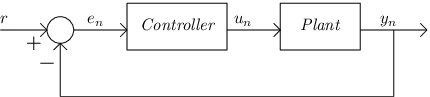
If the controller is an integrator having the transfer function $G_{c}(z)=Az^{-1}/(1-z^{-1})$, for a constant $A>0$, then in the time domain it is defined by the relation $u_{n}=u_{n-1}+Ae_{n-1}$. However, we will consider an adjustable (controlled) gain, and hence the controller equation has the form

$$u_{n}=u_{n-1}+A_{n}e_{n-1},$$

(2)

where the gain $A_{n}$ is computed in a manner described below. The error signal has the form

$$e_{n}=r-y_{n}.$$

(3)

Suppose that the plant functions $g_{n}(u)$ are differentiable, and let “prime” denote their derivatives with respect to $u$. We define the gain $A_{n}$ as

$$A_{n}=\frac{1}{g_{n}^{\prime}(u_{n-1})}.$$

(4)

The systems considered in the sequel have the following structure. Consider a SISO dynamical system having an input $\{u(t)\}$ and output $\{y(t)\}$, $t\geq 0$. Partition the time-horizon $\{t\geq 0\}$ into consecutive time-slots $[\tau_{n-1},\tau_{n})$, $n=1,2,\ldots$, with $\tau_{0}:=0$ and $\tau_{n+1}>\tau_{n}$ $\forall\ n=1,\ldots$; define $C_{n}:=[\tau_{n-1},\tau_{n})$ and call it the $n^{th}$ control cycle. Suppose that the value of the input is changed only at the boundary points $\tau_{n}$, and denote the value of the input $u(t)$ during $C_{n}$ by $u_{n-1}$. Let $y_{n}$ be a quantity of interest that is generated by the system during $C_{n}$ from $u_{n-1}$, such as $y(\tau_{n}^{-})$ or $\int_{C_{n}}y(t)dt$. $y_{n}$ also depends on the initial condition $y(\tau_{n-1})$, but this is reflected in Equation (1) by the system’s definition as time varying. Thus, (1) represents certain input-output properties of dynamical systems while hiding the details of the dynamics and appearing to have the form of a memoryless nonlinearity. Regarding the feedback system, we suppose that $u_{n-1}$, $y_{n-1}$, and $e_{n-1}$ are available to it at time $\tau_{n-1}$, and it generates $y_{n}$ by (1) and computes $A_{n}$ during $C_{n}$ via (4). The closed-loop system is defined by repeated applications of Equations $(1)\rightarrow(4)\rightarrow(2)\rightarrow(3)$.

To see the rationale behind the definition of the gain $A_{n}$ in (4) consider the case where the plant is time invariant, namely $g_{n}(u)=g(u)$ for a function $g:\mathds{R}\rightarrow\mathds{R}$. Then this control law amounts to a realization of the Newton-Raphson method for solving the equation $g(u)=r$, whose convergence means that $\lim_{n\rightarrow\infty}e_{n}=0$. Furthermore, if the derivative $g^{\prime}(u_{n-1})$ cannot be computed exactly, convergence also is ensured under broad assumptions. For instance, suppose that Equation (4) is replaced by

$$A_{n}=\frac{1}{g^{\prime}(u_{n-1})+\xi_{n-1}},$$

(5)

where the error term $\xi_{n-1}$ is due to modeling uncertainties, noise, or computational errors. If the function $g(u)$ is globally monotone increasing or monotone decreasing, and convex or concave throughout $\mathds{R}$, and if the relative error term $|\xi_{n}|/|g^{\prime}(u_{n})|$ is upper-bounded by a constant $\alpha\in(0,1)$ for all $n=1,2,\ldots$, then convergence (in the sense that $\lim_{n\rightarrow\infty}e_{n}=0$) is guaranteed for every starting point $e_{0}$ as long as $g^{-1}(r)\neq\emptyset$. If $g(u)$ is piecewise monotone and piecewise convex/concave then convergence is guaranteed for a local domain of attraction; namely, for every point $\hat{u}\in\mathds{R}$ such that $g(\hat{u})=r$ and $g^{\prime}(\hat{u})\neq 0$, there exists an open interval $I$ containing $\hat{u}$ such that, for every $u_{0}\in I$, $u_{n}\rightarrow\hat{u}$ and hence $e_{n}\rightarrow 0$ as $n\rightarrow\infty$. More specifically, there exist $\gamma\in(0,1)$ and $N\geq 0$ such that, for every $n\geq N$,

$$|e_{n}|\leq\gamma|e_{n-1}|.$$

(6)

These, and more extensive results concerning convergence of Newton-Raphson method for finding the zeros of a function can be found in [21].

In the general time-varying case where the plant function $g_{n}$ is $n$-dependent (as in (1)), it cannot be expected to have $e_{n}\rightarrow 0$. However, the term $\limsup_{n\rightarrow\infty}|e_{n}|$ has been shown to be bounded by quantified measures of the system’s time-variability. For instance, [20] derived the following result under conditions of monotonicity and strict convexity of the functions $g_{n}$: For every $\varepsilon>0$ there exist $\delta>0$ such that, if $|g_{n-1}(u_{n-1})-g_{n}(u_{n-1})|<\delta$ $\forall n=1,2,\ldots$, then $\limsup_{n\rightarrow\infty}|e_{n}|<\varepsilon.$ Moreover, there exist $\eta>0$ and $N\geq 0$ such that, for every $n\geq N$, Equation (6) holds true as long as $|e_{n-1}|>\eta$.

These results have had extensions to the multivariable case arising in Multi-Input-Multi-Output (MIMO) systems with the same number of outputs as inputs (e.g., [21, 22]). Accordingly, for a given $M\geq 1$, let $u\in\mathds{R}^{M}$ and $y\in\mathds{R}^{M}$ denote the input and output of the plant, respectively. Define the plant function by Equation (1) except that $g_{n}$ is a function from $\mathds{R}^{M}$ to $\mathds{R}^{M}$, the feedback equation by (2) except that $A_{n}$ is an $M\times M$ matrix, the error term via Equation (3), and the gain matrix $A_{n}$ by the following extension of Equation (4),

$$A_{n}=\Big(\frac{\partial g_{n}}{\partial u}(u_{n-1})\Big)^{-1}.$$

(7)

In the time-invariant case where $g:=g_{n}$ is independent of $n$, the system consisting of repetitive applications of Equations $(1)\rightarrow(7)\rightarrow(2)\rightarrow(3)$ comprises an implementation of Newton-Raphson method for solving the equation $g(u)=r$.

We are concerned with the time-varying case where the plant function depends on $n$ as in (1), and the Jacobian matrix $\frac{\partial g_{n}}{\partial u}(u_{n-1})$ is approximated rather than computed exactly. In this case Equation (7) is replaced by the following extension of (5),

$$A_{n}=\Big(\frac{\partial g_{n}}{\partial u}(u_{n-1})+\xi_{n-1}\Big)^{-1},$$

(8)

where the error term $\xi_{n-1}$ is an $M\times M$ matrix. Define the relative error at the $n^{th}$ step of the control algorithm by ${\cal E}_{n}:=||\xi_{n-1}||\big(||\frac{\partial g_{n}}{\partial u}(u_{n-1})||\big)^{-1}$. Various general results concerning the Newton-Raphson method guarantee local convergence of the control algorithm under the condition that ${\cal E}_{n}\leq\alpha$ for some $\alpha<1$, for all $n=1,2,\ldots$; see, e.g., [21]. They typically state that $\lim_{n\rightarrow\infty}e_{n}=0$ in the time-invariant case, and show upper bounds on $\lim\sup_{n\rightarrow\infty}||e_{n}||$ in the case of time-varying systems.

The control law defined by Equations (8) and (2) updates all of the $M$ components of $u_{n}$ simultaneously and hence can be viewed as centralized. However, by ignoring the off-diagonal terms of $\frac{\partial g_{n}}{\partial u}(u_{n-1})$ we effectively obtain a distributed controller. Formally, define $D_{n}$ to be the matrix comprised of the diagonal elements of $\frac{\partial g_{n}}{\partial u}(u_{n-1})$, and define $\xi_{n-1}:=D_{n}-\frac{\partial g_{n}}{\partial u}(u_{n-1})$. Then Equation (8) can be computed in parallel by Equation (5) for each input-output coordinate. Thus the system comprised of repeated applications of Equations $(1)\rightarrow(8)\rightarrow(2)\rightarrow(3)$ can be viewed as a distributed system consisting of repeated runs of $(1)\rightarrow(5)\rightarrow(2)\rightarrow(3)$.

This section describes an application of the control technique described in Section II to temperature regulation in computer cores by adjusting their frequencies. Unlike the case of regulating the dynamic power, described in [20], the frequency-to-temperature relationships are highly dynamic and complex, and moreover, the temperatures at various cores on a chip are inter-related. Nevertheless our objective is to have a distributed controller whose required calculations are as simple as possible since, among other reasons, their complexity poses a lower bound on the durations of the control cycles.

To this end we consider approximations that trade off precision with low computational complexity by leveraging the convergence robustness reflected in Equations (5) and (6). Therefore much of the developments in this section concern modeling approximations that yield simple computations. The resultant control law is tested in the next section.

The first part of the investigation concerns the frequency-to-temperature relations in a single core, formalized via the scalar-version of Equation (1). Suppose that the frequency applied to the core has a constant value during each control cycle and it is changed only at the cycle boundaries. Let $\phi$ denote the frequency applied to the core during a typical control cycle, and let $P:=P(t)$ and $T:=T(t)$ denote the resulting dissipated power and spatial average temperature during the cycle. The power has two main components: static power and dynamic power, respectively denoted by $P_{s}$ and $P_{d}$. The static power is dissipated due to leakage currents in the transistors, and the dynamic power is dissipated when the transistors are switched between the on and off states. Figure 2 depicts the functional relations between these quantities, and we note that the dynamic power depends on the frequency, the temperature depends on the total power, and the static power depends on the frequency and temperature. The relationships between these quantities are indicated in the figure by the system-notation $S_{1}$, $S_{2}$, and $S_{3}$, and we next describe their models in detail.

The core frequency typically is controlled by an applied voltage $V$, not shown in Fig. 2. The relationship between frequency and voltage can be modeled by the affine equation

$$V=m\phi+V_{0},$$

(9)

[23, 24] whose slope $m$ often can be obtained from the manufacturer.

As mentioned earlier, the total power is given by

$$P\ =\ P_{s}+P_{d}.$$

(10)

The system $S_{1}$ (Figure 2): An established physical model for the static power is described in [25], and it is given by the equation

	$\displaystyle P_{s}\ =\ VNk_{{\rm design}}I^{\prime}_{so}e^{-(V_{{\rm off}})q/(\eta kT)}$
	$\displaystyle\times 10^{-(V_{T})q/(2.303\eta kT)},$		(11)

where $V$ is the applied voltage, $N$ is the number of transistors in the core, $k_{{\rm design}}$ is a positive parameter depending on the core design, $I^{\prime}_{so}$ is a constant related to the subthreshold drain current, $V_{{\rm off}}$ is an empirically determined model parameter, $q=1.6\times 10^{-19}$C is the electron’s charge, $\eta$ is a technology-dependent parameter, $k=1.38\times 10^{-23}m^{2}kgs^{-2}K^{-1}$ is the Bolzmann’s constant, $T$ is the core temperature in Kelvin, and $V_{T}$ is the threshold voltage of the transistor. Grouping terms and defining

$$\beta=Nk_{{\rm design}}I^{\prime}_{so}$$

and

$$\gamma=q(V_{{\rm off}}+V_{T})/(2.303\eta k),$$

we obtain the equation

$$P_{s}\ =\ V\beta\times 10^{-\gamma/T},$$

(12)

where we note that $\beta>0$ and $\gamma>0$. Observe that $P_{s}$ depends on $V$ (and hence on $\phi$ via (9)) as well as on $T$.

The system $S_{2}$: An established model for the dynamic power [26] is described by the following equation,

$$P_{d}\ =\ \alpha(t)CV^{2}\phi,$$

(13)

where $C$ is the lumped capacitance of the core, and $\alpha(t)$, called the activity factor, is a time-varying parameter related to the amount of switching activity of the logic gates at the core. We note that $\alpha(t)$ cannot be effectively computed or predicted in real time, but its evaluation is not needed for the control algorithm.

The system $S_{3}$: A detailed physical model for the power-to-temperature relationship is quite complicated. However, it will be seen that what we need is the derivative term $\frac{dT}{dP}$, and that this can be approximated by a constant which can be computed off line. In making this approximation we leverage the robustness of the tracking algorithm with respect to errors in the computation of $g_{n}^{\prime}(u_{n-1})$ (see (5),(6)), as discussed in Section II.

The power-to-temperature relationship in a core has had an effective model in [27], that is based on a linear and time-invariant system, and hence yields fast simulation-response time as compared to physics-based models. The dimension of the system is the number of functional units in the core, typically in the $50$ - $100$ range, the input $u$ represents the vector of the dissipated power at each functional unit, and the state variable $x$ is the temperature at each functional unit. The state equation has the form

$$\dot{x}\ =\ Ax+Bu,$$

(14)

where the matrices $A$ and $B$ can be estimated off line. At each time $t$, the total dissipated power at the core, $P:=P(t)$, and the spatial average of the core temperature, $T:=T(t)$, are linear combinations of $u$ and $x$, respectively, and therefore the $P-T$ relationship can be described via the scalar differential equation

$$\dot{T}=aT+bP.$$

(15)

Consequently, the derivative term $\frac{dT}{dP}$ satisfies the equation

$$\frac{d}{dt}\Big(\frac{dT}{dP}\Big)=a\Big(\frac{dT}{dP}\Big)+b.$$

(16)

The constants $a$ and $b$ can be estimated off line via simulation and used to solve the latter equation. Moreover, if the settling time of this equation is shorter than the control cycles then we just use the steady-state value of Equation (16), which is $-\frac{b}{a}$. We feel confident that this additional approximation simplifies the control algorithm without significantly degrading its tracking performance. Details of the computation of this term will be presented in the next section, where its effectiveness in temperature control will be demonstrated.

Using the above models for the systems $S_{1}$, $S_{2}$, and $S_{3}$, we can approximate the derivative term $\frac{dT}{d\phi}$ that is required by the regulation law via Equation (5). In fact, combining Equations (9), (10), (12), and (13), and taking derivatives, we obtain, after some algebra, that

$$\frac{dT}{d\phi}=\frac{\Big(\frac{dT}{dP}\Big)\Big(m\frac{P_{s}}{V}+(P-P_{s})\Big(\frac{1}{\phi}+\frac{2m}{V}\Big)\Big)}{1-\Big(\frac{dT}{dP}\Big)P_{s}(\log 10)\Big(\frac{-\gamma}{T^{2}}\Big)}.$$

(17)

We point out that all of the terms in the RHS of this equation except for $P_{s}$ and $\frac{dT}{dP}$ can be obtained from real-time measurements of a core, $P_{s}$ can be calculated online using Equation (12), and $\frac{dT}{dP}$ can be estimated off-line by its steady-state value, $-\frac{b}{a}$, obtained from (16).

Consider now the case of multiple cores on a chip, where the problem is to regulate their temperatures to given (not-necessary identical) setpoints by adjusting their respective frequencies. Due to the thermal gradients between the cores, it appears that their temperatures have to be regulated jointly. However, extensive simulations, described in the next section, revealed that the Jacobian matrix of the function relating the cores’ frequency vector to the temperature vector is diagonally dominant and this justifies the use of a distributed control where each core runs an adjustable-gain integrator as described in Section II. The details of this control law will be presented in the next section.

We tested the proposed controller on Manifold [28], a cycle-level, full-system processor simulation environment with a suitable interface for injecting the thermal controller. The Manifold framework simulates the architecture-level execution of applications based on state-of-the-art physical models [29]. A functional emulator front-end [30] boots a Linux kernel and executes compiled binaries from an established suite of benchmarks [31].

The processor that we simulated consists of four out-of-order execution cores, a two-level cache hierarchy, and a memory controller, and its architecture is shown in Figure 3. The centralized (joint) control consists of repeated applications of Equations $(1)\rightarrow(8)\rightarrow(2)\rightarrow(3)$, where $u_{n-1}=\phi_{n-1}\in\mathds{R}^{4}$ is the vector of core frequencies during the $n^{th}$ cycle and $y_{n}=T_{n}\in\mathds{R}^{4}$ is the vector of core temperatures at the end of the $n^{th}$ cycle. Recall that Equation (8) denotes the controller’s gain, and since it is diagonal, the control is implemented by the cores in a distributed fashion. In contrast Equation (1) represents the processor system and hence must be simulated jointly. This was done in Manifold in the following way.

Equation (1) can be written as $T_{n}=g_{n}(\phi_{n-1})$, where $\phi_{n-1}:=(\phi_{n-1,1},\ldots,\phi_{n-1,4})^{\top}\in\mathds{R}^{4}$ and $T_{n}:=(T_{n,1},\ldots,T_{n,4})^{\top}\in\mathds{R}^{4}$ according to their respective co-ordinates, with the second subscript $j=1,\ldots,4$ corresponding to the index of the core in Figure 3. In Equation (8) we approximate the $4\times 4$ Jacobian matrix $\frac{dT_{n}}{d\phi_{n-1}}$. Its diagonal terms, $\frac{\partial T_{n,j}}{\partial\phi_{n-1,j}}$, $j=1,\ldots,4$, are just the terms $\frac{dT}{d\phi}$ in the Left-Hand Side (LHS) of Equation (17) with the subscripts $n,j$ indicating core $j$ at the $n^{th}$ control cycle. As mentioned earlier all the terms in the RHS of (17) can be obtained from real-time measurements and computation except for $\frac{dT}{dP}$, now referred to as $\frac{dT_{n,j}}{dP_{n-1,j}}$. For estimating this term we used (16) in the steady state. To this end we ran extensive Manifold simulations of the processor in open loop with various input frequencies. Each simulation was run for successive cycles of $10$ms, long enough for the temperature to reach its steady state, and it yielded traces of power and its corresponding temperature at each cycle. The traces, providing over $4,000$ data pairs per core, indicated a nearly-affine power-to-temperature relation for each core regardless of the physical state (frequencies and temperatures) at the other three cores. We used the MATLAB Curve-Fitting Toolbox to approximate these power-temperature relations by respective lines, whose slopes serve to estimate the terms $\frac{\partial T_{n,j}}{\partial P_{n-1,j}}$. Since the $P$-$T$ traces were generated across the entire spectrum of frequencies at all four cores, the slopes of the approximating lines do not depend on $n$, although they may depend on $j=1,\ldots,4$ according to the processor’s floor plan. Thus, the steady-state solution of Equation (16) in our case has the following approximation,

$$\frac{\partial T_{n,j}}{\partial P_{n-1,j}}\cong-\frac{b_{j}}{a_{j}},\ \ \ \ \ j=1,\ldots,4,$$

(18)

whose right-hand side is the slope of the line associated with core $j$. The MATLAB Curve-Fitting Toolbox yielded the following values, $3.97,5.242,3.877,4.055$ for cores $1-4$, respectively, with an R-Square confidence metric $>0.97$. As a further approximation we averaged these four numbers and thus used $-\frac{b_{j}}{a_{j}}\cong 4.286$ for $j=1,\ldots,4$. This, in conjunction with (17) yields the terms $\frac{\partial T_{n,j}}{\partial\phi_{n-1,j}}$. We note that while this approximation of $\frac{\partial T_{n,j}}{\partial P_{n-1,j}}$ is independent of $n$ or $j$, the partial derivative $\frac{\partial T_{n,j}}{\partial\phi_{n-1,j}}$ does depend on $n$ and $j$ through the other terms in the RHS of (17).

For the off-diagonal terms of $\frac{dT_{n}}{d\phi_{n-1}}$ we observe (by the chain rule) that for $i,j=1,\ldots,4$,

$$\frac{\partial T_{n,i}}{\partial\phi_{n-1,j}}=\frac{\partial T_{n,i}}{\partial T_{n,j}}.\frac{\partial T_{n,j}}{\partial\phi_{n-1,j}}.$$

(19)

The second multiplicative term in the RHS of (19) was discussed in the previous paragraph. As for the first term, we estimated it by finite-difference approximations from the traces of simulation outputs. To this end we used HotSpot, an established simulation platform designed to assess the thermal behavior of digital designs [32]. The thermal model generated by HotSpot consists of a linear, time-invariant circuit comprised of resistors and capacitors, where potentials and currents represent temperature and power, respectively. The input to the circuit consists of current sources and the outputs are node voltages, and hence HotSpot is a suitable tool for modeling the thermal behavior of the core.

Varying the input power to the cores one-at-a-time, we obtained the temperature variations from which the finite-difference approximations for $\frac{\partial T_{n,i}}{\partial T_{n,j}}$ were derived. These approximating terms also are independent of $n$ and hence denoted by $\frac{\partial T_{i}}{\partial T_{j}}$, but $\frac{\partial T_{n,j}}{\partial\phi_{n-1,j}}$ certainly depends on $n$ through the second term in the RHS of (19).²² 2 Manifold has the core frequencies as input but it does not permit us to vary the core powers one-at-a-time, while HotSpot allows us to do just that. This is the reason we used both simulation environments in the manner described above.

The matrix $\frac{\partial T_{i}}{\partial T_{j}}$, $i,j=1,\ldots,4$, thus obtained from HotSpot, is

	$\displaystyle\frac{\partial T_{i}}{\partial T_{j}}=\begin{bmatrix}1\times 10^{6}&0.0439&0.003378&0.003378\\ 0.0439&1\times 10^{6}&0.003378&0.003378\\ 0.003378&0.003378&1\times 10^{6}&0.0439\\ 0.003378&0.003378&0.0439&1\times 10^{6}\end{bmatrix}$
	$\displaystyle\times 10^{-6}.$

This is clearly diagonally dominant, and hence we expected the Jacobian matrix $\frac{dT_{n}}{d\phi_{n-1}}$ to be diagonally dominant as well. This indeed was observed at each value of $n$, as the following randomly-chosen example from our Manifold runs shows,

$$\frac{dT_{n}}{d\phi_{n-1}}=\begin{bmatrix}23800&1109&73.78&72.73\\ 1045&25270&73.78&72.73\\ 80.405&85.37&21870&945\\ 80.405&85.37&958&21530\end{bmatrix}\times 10^{-6}.$$

With this we felt confident in neglecting the off-diagonal terms of the Jacobian matrix, thereby replacing the joint core-temperature control based on Equation (8) by four parallel one-dimensional controllers, one for each core, based on Equation (5).

We implemented the distributed controller in conjunction with Manifold simulation of the processor. Each one of the cores executed a different benchmark program from the parsec suite of benchmarks [31]: blackscholes, swaptions, facesim, and fluidanimate were executed by Core $1$, Core $2$, Core $3$, and Core $4$ (see Figure 3), respectively. The target temperature of all cores was set to $340$K, a typical value, and the range of frequencies was $1$GHz to $4.7$GHz. The control cycles at each one of the controllers were $10$ms. blackscholes running on Core $1$ lasts $400$ms and hence the control was run for $40$ cycles, while the rest of the benchmarks take longer than $700$ms but we graph the results only for the first $70$ control cycles. The results are shown in the four graphs in Figure 4, and for each core we computed the average temperature from the end of the first overshoot to the cycle ending at the final time shown in the graph ($400$ ms for Core $1$, $700$ ms for the other cores).

In Core $1$ we notice convergence at $5$ iterations (control cycles) following a fast rise and a $5$-degree overshoot. The average temperature (from the end of the first overshoot to iteration $40$) is $339.995$K. In Core $2$ we see a similar rise and overshoot as in Core $1$, but then we note an oscillatory behavior and not a smooth tracking. The reason is that the benchmark swaptions had large and rapid variations in its activity factor $(\alpha(t))$ and hence in the dissipated dynamic power, causing ripples in the temperature profile. However, the computed average temperature is $339.96$K - arguably quite close to the target setpoint of 340K.

Core $3$ shows no tracking until $250$ms, then an overshoot followed by a $130$-ms smooth tracking, and a period of minor ripples. The reason for the delayed tracking is that during the first $250$ms the benchmark facesim is in a data-fetch phase when most of the computation units within the core are idle. Therefore there is no significant dynamic power dissipation and the core temperature does not rise. During that phase the core frequency first climbs to its maximum value ($4.7$Ghz) and then stays there until time $250$ms. Once the program enters the computation phase (time $>250$ms), the dynamic power rises which causes the core temperature to increase and the controller is now able to track the set temperature of $340$K. The average temperature, computed as before, was $340.204$K.

In Core $4$ the benchmark program has two data-fetch periods and also periods of wide-range power dissipation during its execution. We discern a similar delayed tracking as was observed with Core 3 but for a shorter duration, ending at $t=80$ms. Later the program enters another data-fetch phase in the time range of $400$ - $500$ms, causing the core temperature to drop while the frequency rises to its maximum value. In both cases the data-fetch phase is followed by a computation phase which results in a temperature overshoot followed by a period of tracking except for ripples that are due to large variability in the dynamic power. The average temperature from the end of the first overshoot to the last control cycle shown in the graph was $339.565$K.

In the previous simulation we allowed the frequency to take any value in the range $1$GHz to $4.7$GHz. However, in a typical processor only a finite set of frequencies can be applied to a core. Therefore we repeated the simulation of the control technique for the following set of allowed frequencies, $\{1,1.5,1.8,3.4,3.7,3.9,4.0,4.1,4.2,4.4,4.7\}$ GHz. The only difference from the previous simulation is that in Equation (2) we took the control $u_{n}$ to be the nearest element in this set to the computed term $u_{n-1}+A_{n}e_{n-1}$. The results are shown in Figure 5, and they are similar to those in Figure 4 except that slightly larger ripples and minor steady-state errors are discerned. These were expected, and are due to the quantization errors in the selection of frequencies. However, the average temperatures at the cores, from the end of the first overshoot to the final time, are quite close to the setpoint reference: $340.482$K, $339.986$K, $340.623$K, and $339.392$K at Cores $1-4$, respectively.

We close this section by comparing the tracking performance of our adaptive-gain controller with those using fixed gains. The need for an adaptive-gain control arises from unpredictable program activity factors $(\alpha(t))$, which may vary widely during the program. We simulated the four-core system but applied the controllers only to core 4 running the fluidanimate benchmark. The frequency range is continuous. We chose a low gain of 10 and a high gain of 120. The graphs of the temperature traces obtained from these two gains as well as the variable-gain control are shown in Figure 6. It is readily seen that the low gain results in the longest settling times, while the high gain yields larger oscillations. Not surprisingly, the tracking performance of the variable-gain controller is better than those of the two fixed-gain controls.

Temperature regulation has emerged as a fundamental requirement of modern and future processors. The state of the practice to date has been dominated by ad-hoc adaptive heuristics. More recent attempts have begun to apply the rich landscape of control theory to this problem. However, these techniques have primarily dealt with temperature as a constraint while controlling power dissipation.

This paper makes a subtle but important observation - temperature ought to be directly regulated to track a target value while power should be managed to maximize performance. Regulating chip-wide temperature to a balanced thermal field is necessary while preventing transitions across a maximum temperature, since the latter can produce thermal fields that adversely affect reliability and performance. Furthermore, unlike prior works we consider a nonlinear, time-varying plant model that explicitly captures the exponential dependence of temperature and static power, and devise a distributed control technique that trades off precision with simplicity of real-time computations. Simulation results using a full system, cycle level simulator executing industry standard benchmark programs indicate convergence of our regulation technique despite the modeling approximations.

References

- [1] R. H. Dennard, F. H. Gaensslen, V. L. Rideout, E. Bassous, and A. R. LeBlanc, “Design of ion-implanted mosfet’s with very small physical dimensions,” Solid-State Circuits, IEEE Journal of, vol. 9, no. 5, pp. 256–268, 1974.
- [2] “International Technology Roadmap for Semiconductors (ITRS), 2011,” http://www.itrs.net/Links/2011ITRS/Home2011.htm, accessed: 2014-03-15.
- [3] K. Skadron, M. R. Stan, W. Huang, S. Velusamy, K. Sankaranarayanan, and D. Tarjan, “Temperature-aware microarchitecture,” in ACM SIGARCH Computer Architecture News, vol. 31, no. 2. ACM, 2003, pp. 2–13.
- [4] K. Skadron, T. Abdelzaher, and M. R. Stan, “Control-theoretic techniques and thermal-rc modeling for accurate and localized dynamic thermal management,” in High-Performance Computer Architecture, 2002. Proceedings. Eighth International Symposium on. IEEE, 2002, pp. 17–28.
- [5] G. Liu, M. Fan, and G. Quan, “Neighbor-aware dynamic thermal management for multi-core platform,” in Design, Automation & Test in Europe Conference & Exhibition (DATE), 2012. IEEE, 2012, pp. 187–192.
- [6] I. Yeo, C. C. Liu, and E. J. Kim, “Predictive dynamic thermal management for multicore systems,” in Proceedings of the 45th annual Design Automation Conference. ACM, 2008, pp. 734–739.
- [7] J. Kong, S. W. Chung, and K. Skadron, “Recent thermal management techniques for microprocessors,” ACM Computing Surveys (CSUR), vol. 44, no. 3, p. 13, 2012.
- [8] J. Donald and M. Martonosi, “Techniques for multicore thermal management: Classification and new exploration,” ACM SIGARCH Computer Architecture News, vol. 34, no. 2, pp. 78–88, 2006.
- [9] H. Qian, X. Huang, H. Yu, and C. H. Chang, “Cyber-physical thermal management of 3d multi-core cache-processor system with microfluidic cooling,” Journal of Low Power Electronics, vol. 7, no. 1, pp. 110–121, 2011.
- [10] B. Shi, Y. Zhang, and A. Srivastava, “Dynamic thermal management for single and multicore processors under soft thermal constraints,” in Proceedings of the 16th ACM/IEEE international symposium on Low power electronics and design. ACM, 2010, pp. 165–170.
- [11] Y. Fu, N. Kottenstette, C. Lu, and X. D. Koutsoukos, “Feedback thermal control of real-time systems on multicore processors,” in Proceedings of the tenth ACM international conference on Embedded software. ACM, 2012, pp. 113–122.
- [12] F. Zanini, D. Atienza, L. Benini, and G. De Micheli, “Multicore thermal management with model predictive control,” in Circuit Theory and Design, 2009. ECCTD 2009. European Conference on. IEEE, 2009, pp. 711–714.
- [13] X. Wang, K. Ma, and Y. Wang, “Adaptive power control with online model estimation for chip multiprocessors,” Parallel and Distributed Systems, IEEE Transactions on, vol. 22, no. 10, pp. 1681–1696, 2011.
- [14] S. Murali, A. Mutapcic, D. Atienza, R. Gupta, S. Boyd, L. Benini, and G. De Micheli, “Temperature control of high-performance multi-core platforms using convex optimization,” in Design, Automation and Test in Europe, 2008. DATE’08. IEEE, 2008, pp. 110–115.
- [15] A. Bartolini, M. Cacciari, A. Tilli, and L. Benini, “Thermal and energy management of high-performance multicores: Distributed and self-calibrating model-predictive controller,” Parallel and Distributed Systems, IEEE Transactions on, vol. 24, no. 1, pp. 170–183, 2013.
- [16] E. Rotem, A. Naveh, D. Rajwan, A. Ananthakrishnan, and E. Weissmann, “Power-management architecture of the intel microarchitecture code-named sandy bridge,” IEEE Micro, pp. 20–27, 2012.
- [17] “AMD Phenom II Key Architectural Features,” http://www.amd.com/us/products/desktop/processors/phenom-ii/Pages/phenom-ii-key-architectural-features.aspx, accessed: 2014-03-15.
- [18] I. Paul, S. Manne, L. Bircher, M. Arora, and S. Yalamanchili, “Cooperative Boosting: Needy vs. Greedy Power Management,” IEEE/ACM International Symposium on Computer Architecture (ISCA), June 2013.
- [19] W. Song, S. Mukhopadhyay, and S. Yalamanchili, “Architectural Reliability: Lifetime Reliability Characterization and Management for Many Core Processors, “ IEEE Computer Architecture Letters, to appear.
- [20] N. Almoosa, W. Song, Y. Wardi, and S. Yalamanchili, “A power capping controller for multicore processors,” in American Control Conference (ACC), 2012. IEEE, 2012, pp. 4709–4714.
- [21] P. Lancaster “Error analysis for the Newton-Raphson method,” in Numerische Mathematik, 1966, vol. 9, pp. 55–68, 1966.
- [22] J. Ortega, and Rheinboldt, C. Werner Iterative solution of nonlinear equations in several variables, Siam, 2000.
- [23] T. D. Burd, T. A. Pering, A. J. Stratakos, and R. W. Brodersen, “A dynamic voltage scaled microprocessor system,” Solid-State Circuits, IEEE Journal of, vol. 35, no. 11, pp. 1571–1580, 2000.
- [24] R. McGowen, C. A. Poirier, C. Bostak, J. Ignowski, M. Millican, W. H. Parks, and S. Naffziger, “Power and temperature control on a 90-nm itanium family processor,” Solid-State Circuits, IEEE Journal of, vol. 41, no. 1, pp. 229–237, 2006.
- [25] J. A. Butts and G. S. Sohi, “A static power model for architects,” in Proceedings of the 33rd annual ACM/IEEE international symposium on Microarchitecture. ACM, 2000, pp. 191–201.
- [26] J. Rabaey, Low Power Design Essentials, ser. Integrated Circuits and Systems. Springer, 2009. [Online]. Available: http://books.google.com/books?id=A-sBy_nmQ8wC
- [27] Y. Han, I. Koren, and C. M. Krishna, “Tilts: A fast architectural-level transient thermal simulation method,” Journal of Low Power Electronics, vol. 3, no. 1, pp. 13–21, 2007.
- [28] Wang et al., “Manifold: A Parallel Simulation Framework for Multicore Systems,” ISPASS, Mar. 2014.
- [29] Song et al., “Energy Introspector: A Parallel, Composable Framework for Integrated Power-Reliability-Thermal Modeling for Multicore Architectures,” ISPASS, Mar. 2014.
- [30] C. D. Kersey, A. Rodrigues, and S. Yalamanchili, “A universal parallel front-end for execution driven microarchitecture simulation,” in Proceedings of the 2012 Workshop on Rapid Simulation and Performance Evaluation: Methods and Tools. ACM, 2012, pp. 25–32.
- [31] C. Bienia, S. Kumar, and K. Li, “Parsec vs. splash-2: A quantitative comparison of two multithreaded benchmark suites on chip-multiprocessors,” in Workload Characterization, 2008. IISWC 2008. IEEE International Symposium on. IEEE, 2008, pp. 47–56.
- [32] “HotSpot Version 5.0” http://lava.cs.virginia.edu/HotSpot/index.htm, accessed: 2014-09-19.