Near-optimal perfectly matched layers
for indefinite Helmholtz problems
Abstract
A new construction of an absorbing boundary condition for indefinite Helmholtz problems on unbounded domains is presented. This construction is based on a near-best uniform rational interpolant of the inverse square root function on the union of a negative and positive real interval, designed with the help of a classical result by Zolotarev. Using Krein’s interpretation of a Stieltjes continued fraction, this interpolant can be converted into a three-term finite difference discretization of a perfectly matched layer (PML) which converges exponentially fast in the number of grid points. The convergence rate is asymptotically optimal for both propagative and evanescent wave modes. Several numerical experiments and illustrations are included.
keywords
Helmholtz equation, Neumann-to-Dirichlet map, perfectly matched layer, rational approximation, Zolotarev problem, continued fractionAMS
35J05, 65N06, 65N55, 30E10, 65D251 Introduction
An important task in science and engineering is the numerical solution of a partial differential equation (PDE) on an unbounded spatial domain. Unbounded spatial domains need to be truncated for computational purposes and this turns out to be particularly difficult when the PDE models wave-like phenomena. In this case the solution may not decay rapidly towards the truncation boundary and artificial reflections and resonances may pollute the numerical solution. The prototype of such notorious PDEs is the Helmholtz equation, which models the propagation of electromagnetic or acoustic fields from a source with a single frequency
| (1) |
As a motivating example from geophysics, this equation may be posed on an unbounded half-space corresponding to the Earth’s subsurface and the variable wave speed may be caused by variations in the sedimental composition, see Figure 1. In seismic exploration a pressure wave signal of frequency is emitted by an acoustic transmitter placed on the Earth’s surface or below, travels through the underground, and is then logged by receivers. From these measurements geophysicists try to infer variations in the wave speed which then allows them to draw conclusions about the subsurface composition. Clearly, the spatial domain for this problem needs to be truncated and there are various ways for achieving this, with a very popular approach being known as perfectly matched layer (PML, see [7, 10, 13]).
A perfectly matched layer can be seen as a localized modification of the spatial discretization scheme to absorb the waves exiting the computational domain. In a finite difference framework such layers typically lead to variable complex-valued step sizes, which is why this approach is sometimes also referred to as complex coordinate stretching. The aim of an efficient PML is to achieve a strong absorption effect by adding only a few number of layers. The aim of this work is to extend a modern finite-difference construction of perfectly matched layers which are near-optimal for indefinite Helmholtz problems, that is, they achieve near-best possible absorption for a given number of layers. The number of required layers is critical in particular for large-scale simulations of three-dimensional exterior problems. A variety of such problems arise, for example, in oil and gas exploration, and near-optimal grids are part of almost all electromagnetic simulators used at Schlumberger [15, 1, 57]. Other applications of effective discretizations of exterior domains include homogenization theory, photonic crystals, energy-driven pattern formation, and the modelling of biologic cell communication (see, e.g., [41, 42, 43]).
1.1 Outline of this work
We will now give a short overview of this work and explain the structure of the paper. Let us start by considering a prototype of a differential equation on an unbounded domain, the two-point boundary value problem
| (2) |
where is nonsingular and . If is a discretization of a differential operator on some spatial domain , then (2) is a semidiscretization of an -dimensional partial differential equation on . Assuming that problem (2) is well posed (which may require some additional conditions like, e.g., the limiting absorption principle discussed below), its exact solution can be given in terms of matrix functions as . In particular, at the solution is given as
| (3) |
The function is often referred to as the impedance function (also known as Weyl function), and it completely characterizes the reaction of the unbounded domain to an external force [36]. The relation (3) allows for the exact conversion of the Neumann data at the boundary into the Dirichlet data , without the need for solving (2) on its unbounded domain. This is why is often referred to as the Neumann-to-Dirichlet (NtD) operator.
When solving wave scattering problems one typically deals with a discretization matrix of the negative shifted Laplacian on . Under the assumption that does not depend on , problem (2) is a semidiscretization of the indefinite Helmholtz equation (1) on the domain . In this case the matrix is (similar to a matrix) of the form
| (4) |
where is Hermitian positive definite, is the identity matrix, and is not in the spectrum of . For a solution of (2) to be unique we impose the limiting absorption principle (see, e.g., [50]). This means that for a real number we define as a limit of solutions of (2) with wave numbers () instead of , i.e.,
| (5) |
This uniquely defines the value , notwithstanding that some eigenvalues of may lie on the standard branch cut of .
We will now outline our construction in the following sections, which combines ideas of the eminent mathematicians Y. I. Zolotarev (1847–1878), T. J. Stieltjes (1856–1894), and M. G. Krein (1907–1989). The main aim in section 2 is to approximate by a rational interpolant of type , so that can be seen as an approximate NtD operator, mapping the Neumann data to the Dirichlet data . Clearly, the weighted 2-norm approximation error of this map is
where and are the eigenpairs of with . We have and thus arrive at the problem of scalar rational approximation of on the union of a positive and a negative real interval. Our rational interpolant is obtained by combining two optimal Zolotarev interpolants constructed for the two intervals separately. For illustration purposes we have graphed the relative error of such a function in Figure 2. In addition to the explicit construction of such approximants, section 2 also contains a novel detailed convergence analysis, with the more technical proofs given in the appendix.
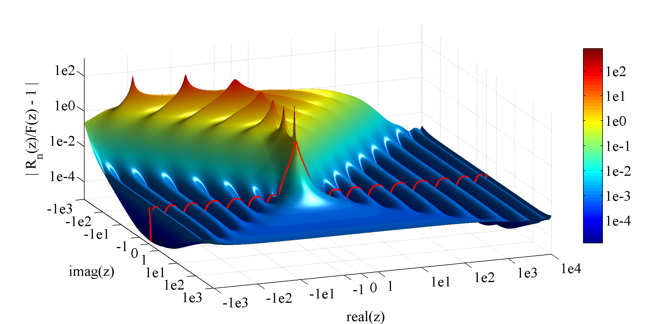
In section 3 we will show that the rational function can be converted into an equivalent three-term finite difference scheme on a nonuniform grid with points. This is achieved by formally rewriting as a Stieltjes continued fraction and using Krein’s interpretation of that fraction as a finite-difference scheme. However, due to the non-Stieltjes nature of (its poles may lie on a curve in complex plane, as shown in Figure 3) the continued fraction coefficients can also be complex, which results in a finite difference scheme with complex-valued grid steps. This scheme allows for the simple and efficient computation of an NtD map and the construction of an absorbing boundary layer for indefinite Helmholtz problems. The near-optimality of implies that the number of required grid points is close to smallest possible. A summary of an algorithm for computing this grid is given in section 4.
Section 5 is devoted to the adaptation of our PML construction to a second-order finite difference framework. In particular, in section 5.1, we extend our optimal rational approximation approach to the infinite lattice problem. Our analysis carries over to this problem, thereby providing a novel theoretical justification for the exponential error reduction in our perfectly matched layer as the number of grid points increases.
Finally, in section 6 we demonstrate the high accuracy and exponential convergence of our perfectly matched layer with several numerical examples.
1.2 Review of related work
It was already shown in [18, 34] that a rational approximant of type for the function can be converted into an equivalent three-term finite difference scheme on a special nonuniform grid with points, mapping the Neumann data to the Dirichlet data . In these papers the authors were mainly concerned with a special instance of (2) where corresponds to a discretization of the negative Laplacian , in which case is a real symmetric positive definite matrix. The error of the approximate Neumann-to-Dirichlet (NtD) map is then bounded by the maximum of on the positive spectral interval of . Approximation theory allows for the construction of exponentially convergent rational functions with a convergence rate weakly dependent on the condition number of , thus producing a three-term finite difference scheme with a so-called optimal grid (also known as finite-difference Gaussian rule or spectrally matched grid). The connection of and this grid is inspired by Krein’s mechanical interpretation of a Stieltjes continued fraction [36]. It was shown in [5] that the same grids produce exponentially convergent NtD maps even for problems arising from the semidiscretization of anisotropic elliptic PDEs and systems with mixed second-order terms, i.e., when the second-order ODE system in (2) is modified by adding a first-order term.
It should be noted that the positive and negative eigenmodes of correspond to so-called evanescent and propagative solutions and , respectively, with denoting the Heaviside step function. The evanescent modes, i.e., the nonzero eigenmodes in the spectral decomposition of , decay exponentially as increases (hence the name). Therefore a simple, though possibly not the most efficient, way to absorb them is to truncate the domain at some (sometimes quite significant) distance from the targeted area of interest, and then to deal with the propagative modes alone. On the other hand, the norm does actually not depend on , so simple boundary truncation will not be effective for absorbing propagative modes.
In their seminal paper [21], Enquist and Majda computed as a Padé approximant of at some real negative point and then evaluated it via continued fraction-type recursions. This approach yielded exponential convergence on the negative real semiaxis, however, with the rate quickly deteriorating towards the origin. Another celebrated approach for absorbing propagative modes is called complex scaling and was originally introduced in [7] for molecular physics calculations. It is also known as perfectly matched layer (PML), a term coined in the influential work [10], where it was independently rediscovered and adapted for time-domain wave propagation. We will use the latter term because it seems to be more established in the wave propagation literature. The well-posedness of the PML formulation was studied in [9, 3]. The essence of the PML approach is a complex coordinate transformation which changes purely imaginary exponentials of propagative modes to complex decaying ones, thus, in principle, allowing reflectionless domain truncation [7, 13]. However, coarse PML discretizations introduce undesirable numerical reflections which decay rather slowly with the grid size in case of low-order discretization schemes. This problem was partially circumvented in [4] for the solution of time-domain wave problems, where the optimal gridding approach was extended to PML discretizations. By choosing an appropriate purely imaginary grid this approach allowed for the construction of all possible rational interpolants for on a real negative interval, including the Padé approximants constructed in [21], and preferably the best uniform approximants targeting the spectral support of the expected solution. See also [39] and [19] for adaptations of the optimal gridding approach to the hyperbolic elasticity system and the Helmholtz equation, respectively. A non-optimal PML layer for absorbing both evanescent and propagative modes in dispersive wave equations has been proposed in [56]. However, the problem of designing discrete PMLs which are optimal for both wave modes remained open.
Our construction in section 2 is inspired by a “trick” originally used by Zolotarev and Newmann, writing the relative approximation error in terms of , where is a polynomial of degree , . This trick was rediscovered in [29, 28], where was identified with the numerical reflection coefficient, and a continued-fraction absorbing condition was explicitly constructed in terms of the roots of and introduced in the PDE discretization via a so-called trapezoid finite element method. However, these important papers fell short of introducing optimal approximants. In addition to the construction of these approximants, section 2 also contains a novel detailed convergence analysis. To make our paper more pleasant to read we have decided to present the technical proofs in an appendix.
In an unfinished report [17], the authors suggested to split into the product of polynomials with real and imaginary roots, thus decoupling the approximation problems on the positive and negative intervals. It was then suggested to apply conventional optimal rational approximants on each of the two intervals, and the resulting error was only determined by the largest error of these two approximants. A drawback of such an approach is that it requires the splitting of the PML grid into two subdomains with nonlocal finite difference stencils at the conjugation interfaces.
2 Construction of a near-optimal approximant on two intervals
The function is commonly defined in the complex plane with the slit . However, in our application we need an analytic continuation of from the positive real semiaxis to in accordance with the limiting absorption principle (5), i.e., attaining the values
and the principal value of the square root for . We will therefore assume in the following that is defined in with the branch cut in the lower half-plane.
Following [17], we now construct a rational interpolant of type to on the union of two real intervals
using solutions of a classical Zolotarev problem on each of the two intervals. In view of the definition (4), these intervals will correspond to the spectral subintervals and (or their estimates), respectively, where .
Separating the odd and even parts of a polynomial of degree , we define polynomials and of degrees and , respectively, such that
| (6) |
The rational function
| (7) |
will be considered as an approximant for on . We have
| (8) |
and thereby obtain an expression of the relative averaged approximation error as
Following [17, Section 2], we can split the approximation problem on into two independent problems on and .
Lemma 1.
Let and be positive integers such that , and let and be polynomials of degrees and with roots on and , respectively. Define
Then
and
Proof.
This lemma immediately follows from the equalities
and reciprocally
∎
Let us consider a single real interval with , and the problem of finding a real monic polynomial of degree (denoted as ) which attains the minimum in the Zolotarev problem
| (9) |
It is known from [58, 40] that this minimizer exists uniquely, that its roots () are located in , and that they are expressible in terms of elliptic integrals. More details are given in the appendix, in particular, formula (32).
We choose positive integers and and introduce the polynomial
| (10) |
of degree . From Lemma 1 we obtain the following result.
Proposition 2.
The polynomial defined in (10) satisfies
It is well known that the classical Zolotarev functions in (9) converge exponentially. Let us denote by the Cauchy–Hadamard convergence rate of , i.e.,
An exact expression of in terms of elliptic integrals is given in (34). For small interval ratios one can derive a simple approximate expression
in terms of elementary functions [34, Appendix A]. This expression shows the weak dependence of the Cauchy–Hadamard convergence rate on the interval ratio .
In view of Proposition 2, and should be chosen to balance the errors of both Zolotarev functions. One way of achieving this is by setting
| (11) |
and
| (12) |
where is chosen to round to the nearest integer. We are now in the position to formulate a near-optimality result for the obtained approximant.
Theorem 3.
Let us denote
| (13) |
Let the polynomial be defined by (10), the polynomials and defined by (6), the rational fraction defined by (7), and . Further let the conditions (12) and
| (14) |
be satisfied. Then the upper relative error bound
| (15) |
holds. On the other hand, if and are arbitrary polynomials of degrees and , respectively, then satisfies the lower error bound
| (16) |
This theorem, whose proof is given in the appendix, implies that the upper error bound for our Zolotarev approximant and the lower bound for the best possible approximant have the same Cauchy–Hadamard convergence rate , i.e., our approximant is asymptotically optimal in the Cauchy–Hadamard sense. As is also demonstrated by the following numerical example (and the corresponding Table 1), the Zolotarev approximant can be worse than the best possible approximant only by a moderate factor. We should point out that, unlike their real counterparts, complex max-norm optimal rational approximation problems are generally not convex and may have non-unique solutions [52]. It therefore seems unlikely that the near-optimality result of Theorem 3 can be improved significantly.
Example 2.1.
Let us, as in Figure 2, consider the problem of approximating by a rational function of type on the union of two intervals . Using the exact formula (34) we calculate
In Table 1 we list the error bounds of Theorem 3 for various values of together with the actual approximation error. The calculations confirm the bounds and show that they are roughly of the same order, i.e., our approximants have relative errors of the same order as the best possible approximants.
The logarithmic surface plot in Figure 3 shows the relative error for the case (the same as in Figure 2). Note how the poles align on a curve in the lower-left quadrant of the complex plane. We speculate that this curve asymptotically (as ) approximates the shifted branch cut of the analytic continuation of into the lower half-plane, and that possesses the so-called S-property (“symmetry property”, see [26, 48, 27]) with respect to . This would imply that the equilibrium charge of the condenser has a logarithmic potential which is (constant and) minimal on over all “attainable” branch cuts. Our experiments also suggested that the curve coincides exactly with the negative imaginary semiaxis in the case of symmetric intervals , and that it approaches the real positive or negative semiaxis for large or small ratios , respectively.
3 Finite difference grids from rational approximants
We now explain how a rational function can be transformed into an equivalent staggered finite difference grid for (2). Assume that we are given primal grid points and steps
and dual grid points and steps
with in both cases. Denote by approximations to the solution of (2) at the primal grid points . Let the first-order finite differences be located at the dual points (. We assume that the following finite difference relations
| (17) | |||||
| (18) |
are satisfied with the convention that . It can be verified by back-substitution that the value specified by these recursive relations can be written as
where is a rational function of type . By construction, is the Schur complement of the submatrix with positive indices of the system (17)–(18). Written as a finite-length Stieltjes continued fraction (S-fraction11 1 We now allow for complex-valued () in (19), which is different from the classical definition of S-fractions with real positive parameters.) this function takes the form
| (19) |
Recalling from above that the exact solution of (2) satisfies , we are apparently left with the problem of determining such that , optimally in some sense. The conversion of Neumann data to Dirichlet data can now be realized by solving a finite difference relation on a grid generated from quantities and () in (19).
The connection between the S-fraction (19) and the finite difference problem (17)–(18) is due to Mark Krein (see, e.g., [36]). He viewed the problem (17)–(18) as a so-called Stieltjes string, which is a string of point masses and weightless stiffnesses (), both real positive. There is a one-to-one correspondence between the set of Stieltjes strings and Stieltjes spectral functions , which are rational functions of type having non-coinciding real negative poles and real positive residues. For this case, the S-fraction parameters and () can be computed via steps of the Euclidean polynomial division algorithm (see, e.g., [33]), which can be stably executed with the help of the reorthogonalized Lanczos algorithm [18]. The optimal rational approximation of on a positive real interval is a Stieltjes problem [34], hence the generated grid steps are real positive. The approximation problem on a single negative interval can be solved by using , where is the approximation on the symmetrically reflected positive interval. This reflection rotates the grid steps and () by an angle of in , i.e., it makes the grid steps purely imaginary. Generally, the problem of optimal approximation on the union of a positive and a negative interval leads to non-Stieltjes rational functions of type . Assuming absence of breakdowns (which are unlikely but can not be definitely excluded), the transformation to the non-Stieltjes rational function (19) can still be carried out via the complex -step Euclidean algorithm. We used the bi-Lanczos extension of the Lanczos-based algorithm [18] which, according to our experience, always produced meaningful results.
Example 3.1.
We begin with reproducing a real optimal grid from (19) generated for a real positive interval , see Figure 4 (left). Similar results were reported in [34]. We can consider this example as a degenerate case of the two-interval problem with and . The plot shows “alternation” of the primal and dual grid points and monotonically growing steps. The grid looks like an equidistant grid stretched by a rather smooth transform. It was shown in [34] that for large and small interval ratios such transforms are asymptotically close to the exponential.
In Figure 4 (right) we plot the complex finite difference grid points obtained from the continued fraction (19) in the case when and and . We notice the “alternation” of the primary and dual points on some “curve”, which is an intuitive evidence of a good quality of the grid, i.e., we can speculate that the finite difference solution approximates the exact solution with second-order accuracy on that curve. This curve can be interpreted as the complex PML transform of the real positive axis in accordance with [7, 13].
In summary, we observe that the finite-difference operators on grids obtained from (19) approximate the second-order derivative operator on curves in the complex plane. This can be viewed as a complex extension of Krein’s results on the convergence of the Stieltjes discrete string with impedance to its continuous counterpart with impedance when on [36]. Besides internal beauty, this phenomenon may have useful consequences. For example, it lets us hope that pseudospectral estimates and stability results for continuous PMLs and damped 1D differential operators [3, 9, 16] remain valid for (17)–(18) with the optimal grid.
4 Summary of the algorithm
In the following we provide a step-by-step description for computing the grid steps and () in (19).
- 1.
It follows from (8) that the numbers
are the interpolation nodes for as an interpolant of . Knowing interpolation nodes and function values, we compute the coefficients of and by means of solving the corresponding system of linear algebraic equations in high-precision arithmetic.
- 2.
The poles of the interpolant, i.e., the roots of , can be computed as the eigenvalues of an associated companion matrix, see [24, Subsection 7.4.6]. To solve this eigenvalue problem we use the quasi-version22 2 I.e., we formally use in the complex case the formulas intended for the real case. of the QR transformation method [45, § 11.6] and then, if necessary, correct the roots by means of a combination of Laguerre’s [45, § 9.5] and Newton’s [37] method.
- 3.
Knowing the poles of , the corresponding residues are computed.
- 4.
Finally, the grid steps and () are computed using the recursion formulas [18, (3.4)], with the underlying analogue of an inverse eigenvalue problem for a symmetric tridiagonal matrix (see [18, subsection 3.1, item 3∘], [46, theorem 7.2.1]) being solved by a quasi-Lanczos process [14, Ch. 6] with quasi-reorthogonalization. Here we used the well-known connection between the Lanczos and Euclidean algorithms (see, e.g., [33]).
5 Adaptation to a second-order finite difference framework
5.1 Approximation of the discrete impedance function
So far we have considered the function , which arises when solving the boundary-value problem (2) for . When this problem is seen as an infinite extension of some interior computational domain, the exponential convergence of the interpolant is consistent with a high-order (or even spectral) discretization of the operator acting in this computational domain.
However, it is also possible to compute the NtD map of a discretized version of (2) on a uniform infinite grid via rational approximation of a slightly modified function to be determined below. This function will lead to a three-term finite difference scheme which is appropriate for being combined with a standard second-order finite difference discretization in the interior computational domain, because it allows for the elimination of spurious reflections from the PML boundary due to the error of the interior discretization.
Given a fixed step size , let us consider the problem (17)–(18) on the infinite equidistant grid with and for . We will determine a function such that
via a well-known approach widely used in the representation of irrational numbers via continued fractions (see, e.g., [20, section 9]). This approach was already applied in [51] to the infinite lattice problem: the infinite-length S-fraction representation of analogous to (19) is
(for a proof of convergence we refer to [49] or [35, theorem 4.58]). The remainder continued fraction
evidently satisfies the equation
or equivalently . Since , we have arrived at the quadratic equation
We choose the root which converges to the exact impedance as , i.e.,
| (20) |
This function, which we will refer to as the discrete impedance function, approximates with second-order accuracy the exact impedance at the boundary, so being centered, the resulting finite difference scheme is of second order globally.
Analogously to what we had achieved with (3) for continuous , the relation (20) allows us to convert the Neumann data at into the Dirichlet data without actually solving the infinite lattice problem.
For a given let us define . The invertible linear fractional change of variables
| (21) |
translates the union of a negative and a positive segment again into the union of a negative and a positive segment. Let us assume33 3 As discussed earlier, the parameter should be set to a lower bound of ’s spectral interval, in which case the condition corresponds to the Nyquist sampling criterion of two grid points per wave length. This assumption should be met by any reasonable discretization scheme. that . Let denote the rational approximant of theorem 3 for the image of under transformation (21). Then
is small on , the numerator and the denominator
being polynomials of degrees and , respectively. We have thereby established a direct relation between the errors of the rational interpolants for and on transformed compact sets, respectively, with the interpolation nodes being transformed accordingly. This allows us to conclude that we obtain identical convergence rates for both interpolation processes. In particular, Theorem 3 holds with being replaced by .
We would like to mention that a rational approximation-based absorbing boundary condition for the infinite lattice was suggested in [51] and combined with a trapezoidal finite element approach in [29]. However, that approach required a modification of the Helmholtz equation by a higher-order term. On the contrary, in our framework the discreteness can be incorporated simply by adjusting the PML grids. Visually these grids look very similar to the ones shown in Figure 4, i.e., we can speculate again that they approximate the exact solution of (2) with second-order accuracy on some modified -curve in the complex plane.
5.2 Matching interior and exterior discretizations via a single grid
Let us consider the second-order infinite equidistant finite difference problem
| (22) |
with boundary conditions
| (23) |
assuming for . Problem (22) can be split equivalently into an interior finite-dimensional system
| (24) | |||||
and an exterior infinite system
| (25) | |||||
both systems being coupled via a vector variable .44 4 Problem (22)–(23) can be viewed as the second-order discretization of , for some regular enough supported on . As the infinite exterior problem (25) approximates with second-order accuracy the same equation on with conditions and , the relation (24) approximates with second order the same equation restricted to with conditions and .
Problem (25) (with the condition at infinity) was already considered in section 5.1, and can be exactly eliminated using the discrete impedance function (20),
This formally corresponds to a Schur complement. Upon substitution we arrive at the approximate problem
Hence
since all the involved linear systems are well posed uniformly in .
Performing similar manipulations with the approximate problem in reverse order, we obtain the equivalent system (26)–(27)
| (26) | |||||
| (27) | |||||
by introducing and fictitious variables with positive subindices which, unlike their negative counterparts, do not approximate corresponding components of . Finally, eliminating we can merge the systems (26)–(27) into a single recursion
with the convention that for , for , for , for , and (see also Figure 5). This finite difference scheme is easy to implement by simply modifying the trailing primal and dual grid steps in a given finite difference scheme with step size . We reiterate that this scheme converges exponentially with error to the solution of (22)–(23) in the interior domain, i.e., for the nonpositive subindices.
The above derivation can easily be extended to variable operators in the interior domain and tensor-product PML discretizations. This will be illustrated by a numerical example in section 6.2.
6 Numerical experiments
6.1 Waveguide example
To test the accuracy of our absorbing boundary layer, we consider the inhomogeneous Helmholtz equation
on a rectangular domain of length and height . We prescribe homogeneous Dirichlet conditions at the upper and lower boundaries in . The source term is set to
with the Dirac delta function .
Our aim is to verify that our absorbing boundary layer models the correct physical behavior. To this end we solve the above Helmholtz equation on two rectangular domains with fixed height and different lengths and , respectively. See also Figure 7 (left and right, respectively). The wave number is chosen as . The problem is discretized by central finite differences with step size in both coordinate directions. The eigenvalues of the resulting tridiagonal matrix , corresponding to the operator on with homogeneous Dirichlet boundary conditions, are explicitly known and eigenvalue inclusion intervals are
We extend the interior finite difference grid by our absorbing boundary layer with additional grid points to the left of and to the right of , with the near-optimal grid steps computed from a rational interpolant of as explained in section 5.1. The physical domain can hence be thought of as an infinite strip parallel to the -axis. We therefore expect the solutions of both problems (with and ) to coincide when they are restricted to . Visually, this is indeed the case, as one can see in Figure 7 (where ). Note how the amplitude of the solution is damped very quickly inside the absorbing boundary layer.
To quantify the accuracy of our absorbing boundary layer numerically, we plot in Figure 7 the relative uniform norm of the difference of the two numerical solutions and restricted to , i.e.,
| (28) |
Indeed, this figure reveals exponential convergence with the rate given in Theorem 3. In this example, the expected rate is and this is indicated by the slope of the dashed line in Figure 7.
We would like to mention that absorbing boundary layers usually require some physical separation from the support of the right-hand side (the source term) [32]. However, thanks to the efficient absorption of evanescent and propagative modes even on spectral subintervals with extreme interval ratios, we are able to place our Dirac source extremely close to the PML boundary (only one grid point away, see the right of Figure 7) without deteriorating convergence (see Figure 7).


6.2 PML in multiple coordinate directions
In this experiment we demonstrate how our perfectly matched layer can be used to mimic domains which are unbounded in several coordinate directions, and where there is a nonconstant wave speed. To this end consider
on a square domain . The wave speed varies as indicated in Figure 1, with in the gray region (background material), in the light gray layer, and in the dark inclusion at the bottom (see also Figure 9). The wave number is chosen as and the source term is set to
The domain is discretized by central finite differences with step size in both coordinate directions. We aim to append absorbing boundary layers with grid points at each of the four edges of .
For constructing the absorbing layers in the -direction (below and above ) we need inclusion intervals for the negative and positive eigenvalues of , where is the discretization of on with homogeneous Dirichlet boundary and for . (Note that varies only tangentially along the boundaries of , so for we can indeed write .) Possible inclusion intervals for the eigenvalues are
| (29) |
For constructing the absorbing layers in the -direction (to the left of and to the right of ) we need inclusion intervals (29) for the negative and positive eigenvalues of , where is the finite difference discretization of on with homogeneous Dirichlet boundary and
Possible intervals are
| (30) |
From the union of intervals in (29) and (30) we can now calculate the grid steps of absorbing boundary layers in the - and -directions, and then modify the finite difference matrices to and , respectively. As in the previous example, this is done by computing a rational interpolant of defined in section 5.1.
However, there is a small subtlety one has to be aware of with the approach just described: effectively, the NtD operators are now given as and , respectively, and the involved matrices are no longer Hermitian. In Figure 9 (left) we show the eigenvalues of and , respectively, and observe that these eigenvalues have “lifted off” the real axis into the upper half of the complex plane, in agreement with the analysis of [16] for continuous one-dimensional damped operators. From Figure 3 we find at least visually that the Zolotarev approximant is of a good quality in this region as well, and the accuracy of the resulting absorbing boundary layers should still be satisfactory.
To quantify the accuracy numerically, we solve the same Helmholtz problem on a smaller domain , again appended with absorbing boundary layers of grid points at each of the four edges of . As the source term is supported inside , we expect coinciding solutions and on their restrictions to . In Figure 9 (right) we have plotted the relative uniform norm of the difference of both solutions, i.e.,
| (31) |
Again we observe exponential convergence, and the reduction of the measured error is in good agreement with (even slightly better than) the rate expected from Theorem 3.


7 Summary, generalizations, and open problems
We have presented a new approach for the construction of discrete absorbing boundary layers for indefinite Helmholtz problems via complex coordinate transforms. This approach is based on the use of near-optimal relative rational interpolants of the inverse square root (or a modification thereof) on a negative and a positive real interval. Bounds for the approximation error have been derived, and the exponential convergence of the approximants has been established theoretically and demonstrated at numerical examples. Although our focus in this paper was on absorbing boundary conditions for indefinite Helmholtz problems, it was recently understood that these conditions also constitute good approximations to Schur complements of certain PDE discretization matrices, and they became a crucial component of modern Helmholtz preconditioners, such as Schwarz domain decomposition [23, 12] and the sweeping preconditioner in [22]. Preliminary results have shown successful application to a multilevel domain decomposition preconditioner, and a related Schlumberger patent application is pending.
7.1 Time-domain problem
Classical (explicit) finite-difference time-domain formulations lead to PMLs that can be represented via grid steps and which are dependent on the wave number as , , where are real positive parameters [3, 10, 9, 13]. Our experiments suggest that the steps of our optimal PML grids always have positive real parts, and negative or zero imaginary parts; see, e.g., the grid in Figure 4. So formally, the steps of the frequency-dependent PML can be obtained as , , where the steps and are obtained for a fixed wave number . If the rational approximant for uses symmetric intervals of approximation, the corresponding grid lies on a semiaxis rotated by with respect to and the introduction of is equivalent to the rotation of the grid and the spectral measure respectively on and . Therefore such grids retain the exponential convergence for . However, it is not clear if the exponential convergence holds for nonsymmetric intervals, neither is known if this convergence holds for the approximation of the discrete impedance function from section 5.1.
Alternatively, the time domain solution can be represented via stability-correcting functions of the discretized operator with the PML obtained for a fixed wave number; see [19]. It can then be efficiently computed in the time domain via Krylov subspace projection.
7.2 Maxwell and elasticity systems
Important hyperbolic systems, such as isotropic Maxwell’s and linear elasticity systems are usually approximated via staggered finite-difference (finite volume) schemes [55, 53]. Staggered schemes for multidimensional problems can be constructed via tensor products of one-dimensional staggered schemes. Thus the one-dimensional staggered grids developed in this paper can be automatically implemented in such framework, similar to what was done in [15, 39] for PMLs based on the single interval rational approximants. Work [39] also provides error estimates for the propagative modes in isotropic elasticity systems, showing that for hyperbolic systems one may need rational approximants on slightly larger spectral intervals compared to the scalar wave equation.
7.3 Adaptive grids
The uniform approximation approach requires bounds for the smallest/largest negative and positive eigenvalues, which can be rather loose due to the weak dependence of the convergence rate of the Zolotarev approximants on the interval ratios. The external bounds of the intervals can thus be estimated roughly. Still, the numerical estimation of the internal bounds can be rather difficult, and accidentally at least one eigenvalue may be very close to the origin, in which case even an optimal approximant may require significant order for a satisfactory accuracy. To circumvent this problem, it would be interesting to derive a parameter-free near-optimal rational approximant of , which takes into account the discrete nature of the spectrum of and the spectral weights of the vector . Promising steps have been made by using adaptive rational Krylov algorithms [31, 30, 11] for this purpose.
7.4 Variable coefficients
As explained in this paper, variable PDE coefficients in the tangential direction can be straightforwardly incorporated into the PML by modifying . Moreover, according to preliminary findings, our PML approach may be generalized for coefficients varying in the normal direction. Let us replace the first equation of (2) by
with compactly supported coefficient . Then grid steps , can be obtained via rational approximation of the “fine grid” finite-difference NtD map , involving the finite-difference system
with boundary conditions (23). For constant such an approach yields being the same as defined in section 5.1. Our experiments with discrete PMLs for variable coefficients exhibited exponential convergence albeit at a slower rate than for the constant coefficient problem.
7.5 Connection to inverse problems
Constructing PMLs can be viewed as finding equivalent media matching the NtD maps, and this is reminiscent to what is done in inverse problems of electrical impedance tomography (EIT). In fact, the conversion of rational approximations to finite-difference schemes (and its planar generalization) was the basis for the solution of EIT inverse problems via resistor network approximations [8].
Finally, we would like to point out that cloaking problems (which are popular in the inverse problems community) are closely related with the construction of PMLs, because the latter can be viewed as cloaking of the point at infinity. Cloaking problems can also be formulated via complex coordinate transforms [38] and lead to approximation problems of NtD maps. Although the involved Stieltjes impedance function is typically different in these applications, techniques similar to those presented in this paper may still be applicable.
Acknowledgments
We are grateful to Paul Childs, Martin Gander, Mikhail Zaslavsky, and Hui Zhang for useful discussions. We thank the anonymous referees for helpful comments and suggestions, and David Bailey for making available the Fortran 90 multiprecision system [6].
Appendix A Zolotarev approximation and proof of Theorem 3
The solution of the Zolotarev problem (9) can be computed as
| (32) |
where
is the complete elliptic integral of the first kind55 5 The definition of is not consistent in the literature. We stick to the definition used in [44, Ch. VI]. In Matlab one would type ellipke(delta^2) to obtain the value . and where the Jacobian elliptic function is defined via another such function, , by the relations
In order to prove near-optimality results, we first need to study the quantity in (9) carefully. Evidently, . Upper and lower bounds for (9) were given in [40] as
| (33) |
with
Hence the Cauchy–Hadamard convergence rate can be computed as
| (34) |
Recalling the equalities (11) and (13), let us define the sets
and consider the following auxiliary problem: find a (complex) monic polynomial of degree being the minimizer of
| (35) |
We now construct an approximate solution of this problem and show that the approximate solution gives the maximum in (35) which yields the best possible functional value up to a moderate multiplier.
Accounting, as it was done in [17, Section 2], that
and
because these polynomials have real coefficients, the polynomial defined in (10) satisfies
| (36) |
and
| (37) |
Lemma 4.
The polynomial defined in (10) satisfies the inequality
| (38) |
with the numbers and defined in (11) and (13), provided that are chosen according to (12).
On the other hand, for any complex polynomial we have
| (39) |
Proof.
Let be defined as in (10) and conditions (12) be satisfied. Accounting for (36), (37) and (33), we obtain
which gives assertion (38).
To prove assertion (39), we consider the third Zolotarev problem in the complex plane for the condenser (see [25], [54, § 8.7] or [47, § VIII.3]). Due to the symmetry of the condenser, the two measures forming the (unique) equilibrium pair for are symmetric to each other in the evident sense. Thus, one can choose an (in the Cauchy–Hadamard sense) optimal sequence of type rational functions of the form , , such that the roots () of each polynomial belong to . Define
By virtue of (33) and the location of the roots we have
and
whence
Since the quantity under the conditions , , is minimal at
we obtain
so
It follows in view of [25, Theorem 1, Formula (12)] that the logarithmic capacity of our condenser satisfies
Moreover, [25, Theorem 1, Formula (11)] yields for all
from which (39) follows. ∎
We are now prepared to conclude the proof of Theorem 3.
References
- [1] A. Abubakar, T. M. Habashy, V. L. Druskin, L. Knizhnerman, and D. Alumbaugh, 2.5D forward and inverse modeling for interpreting low-frequency electromagnetic measurements, Geophysics, 73:4 (2008), pp. F165–F177.
- [2] N. I. Akhiezer, Theory of Approximation, Dover, 1992.
- [3] D. Appelö, T. Hagstrom, and G. Kreiss, Perfectly matched layers for hyperbolic systems: General formulation, well-posedness, and stability, SIAM J. Appl. Math., 67 (2006), pp. 1–23.
- [4] S. Asvadurov, V. Druskin, M. Guddati, and L. Knizhnerman, On optimal finite-difference approximation of PML, SIAM J. Numer. Anal., 41 (2003), pp. 287–305.
- [5] S. Asvadurov, V. Druskin, and S. Moskow, Optimal grids for anisotropic problems, Electron. Trans. Numer. Anal., 56 (2007), pp. 55–81.
- [6] D. N. Bailey, A Fortran-90 based multiprecision system, RNR Technical Report RNR-94-013, NAS Scientific Computation Branch, NASA, Ames Research Center, CA, USA (1994).
- [7] E. Balslev and J. Combes, Spectral properties of many body Schrödinger operators with dilation analytic interactions, Commun. Math. Phys., 22 (1971), pp. 280–294.
- [8] L. Borcea, V. Druskin, F. Guevara Vasquez and A. Mamonov, Resistor network approaches to electrical impedance tomography, in Inverse Problems and Applications: Inside Out II. Vol. 60. Cambridge University Press, 2013, pp. 55–119
- [9] E. Becache and P. Joly, On the analysis of Berenger’s perfectly matched layers for Maxwell’s equations, Math. Model. Num. Anal., 36 (2002), pp. 87–119.
- [10] J. P. Berenger, A perfectly matched layer for the absorption of electromagnetic waves, J. Comp. Phys., 114 (1994), pp. 185–200.
- [11] M. Berljafa and S. Güttel, Generalized rational Krylov decompositions with an application to rational approximation, The University of Manchester, MIMS Eprint 2014.59, 2014.
- [12] Y. Boubendir, X. Antoine, and C. Geuzaine, A quasi-optimal non-overlapping domain decomposition algorithm for the Helmholtz equation, J. Comp. Phys., 231 (2012), pp. 262–280.
- [13] W. Chew and B. Weedon, A 3D perfectly matched medium from modified Maxwell’s equations with stretched coordinates, Microwave Opt. Technol. Lett., 7 (1994), pp. 599–604.
- [14] J. Cullum and R. A. Willoughby, Lanczos Algorithms for Large Symmetric Eigenvalue Computations. Volume 1, Theory, SIAM, Philadelphia, 2002.
- [15] S. Davydycheva, V. Druskin, and T. Habashy, An efficient finite-difference scheme for electromagnetic logging in 3D anisotropic inhomogeneous media, Geophysics, 68 (2003), pp. 1525–1536.
- [16] T. A. Driscoll and L. N. Trefethen, Pseudospectra for the wave equation with an absorbing boundary, J. Comput. Appl. Math., 69 (1996), pp. 125-142.
- [17] V. Druskin, M. Guddati, and T. Hagstrom, On generalized discrete PML optimized for propagative and evanescent waves, arXiv:1210.7862v1 [math.NA], 29 Oct 2012.
- [18] V. Druskin and L. Knizhnerman, Gaussian spectral rules for the three-point second differences: I. A two-point positive definite problem in a semiinfinite domain, SIAM J. Numer. Anal., 37 (1999), pp. 403–422.
- [19] V. Druskin and R. Remis, A Krylov stability-corrected coordinate-stretching method to simulate wave propagation in unbounded domains, SIAM J. Sci. Comput., 35 (2013), pp. 313–357.
- [20] S. Elaydi, An Introduction to Difference Equations, Springer, New York, 2005.
- [21] B. Engquist and A. Majda, Radiation boundary conditions for acoustic and elastic wave calculations, Comm. Pure Appl. Math., 32 (1979), pp. 313–357.
- [22] B. Engquist and L. Ying, Sweeping preconditioner for the Helmholtz equation: hierarchical matrix representation, Comm. Pure Appl. Math., 64:5 (2011), pp. 697–735.
- [23] M. Gander, Optimized Schwarz methods, SIAM J. Numer. Anal., 44:2 (2006), pp. 699–731.
- [24] G. H. Golub and C. F. van Loan, Matrix computations, The Johns Hopkins Univ. Press, Baltimore and London, 1989.
- [25] A. A. Gonchar, Zolotarev problems connected with rational functions, Math. Digest (Matem. Sbornik), 7 (1969), pp. 623–635.
- [26] A. A. Gonchar, The rate of rational approximation of analytic functions, Proc. Steklov Inst. Math., 166 (1984), pp. 52–60.
- [27] A. A. Gonchar and E. A. Rakhmanov, Equilibrium distributions and degree of rational approximation of analytic functions, Sb. Math., 176 (1987), pp. 306–352.
- [28] M. N. Guddati and K.-W. Lim, Continued fraction absorbing boundary conditions for convex polygonal domains, Int. J. Numer. Meth. Engng., 66 (2006), pp. 949–977.
- [29] M. Guddati and J. Tassoulas, Continued-fraction absorbing boundary conditions for the wave equation, J. Comp. Acoust., 8 (2000), pp. 139–156.
- [30] S. Güttel, Rational Krylov approximation of matrix functions: Numerical methods and optimal pole selection, GAMM-Mitt., 36:1 (2013), pp. 8–31.
- [31] S. Güttel and L. Knizhnerman, A black-box rational Arnoldi variant for Cauchy–Stieltjes matrix functions, BIT Numer. Math., 53:3 (2013), pp. 595–616.
- [32] T. Hagstrom and T. Warburton, Complete radiation boundary conditions: minimizing the long time error growth of local methods, SIAM J. Numer. Anal., 47:5 (2009), pp. 3678–3704.
- [33] O. Holtz and M. Tyaglov, Structured matrices, continued fractions, and root localization of polynomials, SIAM Rev., 54:3 (2012), pp. 421–509.
- [34] D. Ingerman, V. Druskin, and L. Knizhnerman, Optimal finite difference grids and rational approximations of the square root, I. Elliptic problems, Comm. Pure Appl. Math., 53 (2000), pp. 1039–1066.
- [35] W. B. Jones and W. J. Thron, Continued Fractions. Analytic Theory and Applications, Enc. of Math. and its Appl., v. 11, Addison-Wesley P. C., London et al., 1980.
- [36] I. S. Kac and M. G. Krein, On the spectral functions of the string, Amer. Math. Soc. Transl., 103 (1974), pp. 19–102.
- [37] C. T. Kelley, Solving nonlinear equations with Newton’s method, Fundamentals of Algorithms, No. 1, SIAM, Philadelphia, 2003.
- [38] R. V. Kohn, D. Onofrei, M. S. Vogelius and M. Weinstein, Cloaking via change of variables for the Helmholtz equation, Comm. Pure Appl. Math., 63 (2010), pp. 973–1016.
- [39] V. Lisitsa, Optimal discretization of PML for elasticity problems, Electron. Trans. Numer. Anal., 30 (2008), pp. 258–277.
- [40] A. A. Medovikov and V. I. Lebedev, Optimization of stable Crank–Nicolson method, Russian J. Numer. Anal. Math. Modelling, 20 (2005), pp. 283–304.
- [41] F. Posta, S. Y. Shvartsman and C. B. Muratov, Compensated optimal grids for elliptic boundary-value problems J. Comput. Phys. 227 (2008), pp. 8622–8635.
- [42] C. B. Muratov and V. V. Osipov, Optimal grid-based methods for thin film micromagnetics simulations, J. Comput. Phys. 216 (2006), pp. 637–653.
- [43] C. B. Muratov and S. Y. Shvartsman Boundary homogenization for periodic arrays of absorbers, Multiscale Model. Simul. 7 (2008), pp. 44–61.
- [44] Z. Nehari, Conformal mapping, Dover, New York, 1975.
- [45] W. H. Press, S. A. Teukolsky, W. T. Vetterling, and B. P. Flannery, Numerical Recipes in Fortran 77: The Art of Scientific Computing, Cambridge Univ. Press, Cambridge, 1992.
- [46] B. N. Parlett, The Symmetric Eigenvalue Problem, Prentice-Hall, SIAM, Philadelphia, 1998.
- [47] E. B. Saff and V. Totik, Logarithmic Potentials with External Fields, Springer, Berlin, 1997.
- [48] H. Stahl, Orthogonal polynomials with complex valued weight function, I, Constr. Approx., 2 (1986), pp. 225–240.
- [49] T. J. Stieltjes, Recherches sur les fractions continues, Annales de la Faculté des Sciences de Toulouse, 8 (1984), p. 1–122, 9 (1894), p. 1–47.
- [50] M. E. Taylor, Partial Differential Equations II. Qualitative Studies of Linear Equations, Springer, New York, 1996.
- [51] S. Thirunavukkarasu and M. N Guddati, Absorbing boundary conditions for time harmonic wave propagation in discretized domains, Comput. Methods Appl. Mech. Engrg., 200:33 (2011), pp. 2483–2497.
- [52] R. Varga, Scientific computation on mathematical problems and conjectures, CBMS-NSF, SIAM, 1990.
- [53] J. Virieux, P-SV wave propagation in heterogeneous media: Velocity-stress finite-difference method, Geophysics, 51 (1986), pp. 889–901.
- [54] J. L. Walsh, Interpolation and Approximation by Rational functions in the Complex Domain, AMS, Rhode Island, 1960.
- [55] K. S. Yee, Numerical solution of initial boundary value problems involving Maxwell’s equations in isotropic media. IEEE Trans. Antennas Propag., 14 (1966), pp. 302–307.
- [56] M. A. Zahid and M. N. Guddati Padded continued fraction absorbing boundary conditions for dispersive waves, Comput. Methods Appl. Mech. Engrg., 195 (2006), pp. 3797–3819.
- [57] M. Zaslavsky, V. Druskin, S. Davydycheva, L. Knizhnerman, A. Abubakar, and T. Habashy, Hybrid finite-difference integral equation solver for 3D frequency domain anisotropic electromagnetic problems, Geophysics, 76:2 (2011), pp. F123-F137.
- [58] Y. I. Zolotarev, Collection of Works, Saint Petersburg Academy of Sciences, 30:5, 1877.