Optimal stopping for Lévy processes
with polynomial rewards

Ernesto Mordecki Note: Universidad de la República, Facultad de Ciencias, Centro de Matemática. Iguá 4225, 11400 Montevideo, Uruguay. e-mail: mordecki@cmat.edu.uy Yuliya Mishura Note: National Taras Shevchenko University of Kyiv, Department of Probability Theory, Statistics and Actuarial Mathematics. Volodymirska 60, 01601 Kyiv, Ukraine. e-mail: myus@univ.kiev.ua.

Abstract

Explicit solution of an infinite horizon optimal stopping problem for a Lévy processes with a polynomial reward function is given, in terms of the overall supremum of the process, when the solution of the problem is one-sided. The results are obtained via the generalization of known results about the averaging function associated with the problem. This averaging function can be directly computed in case of polynomial rewards. To illustrate this result, examples for general quadratic and cubic polynomials are discussed in case the process is Brownian motion, and the optimal stopping problem for a quartic polynomial and a Kou’s process is solved.

Keywors: Optimal stopping, Lévy processes, polynomial rewards

AMS MSC: 60G40

1 Introduction

Since the seminal work of Darling, Liggett and Taylor (1972), giving the solution to the optimal stopping problem for random walks, and reward functions of the form $g(x)=x^{+}$ and $g(x)=(e^{x}-1)^{+}$ , in terms of the distribution of the maximum of the random walk, it became clear the possibility of linking these two relevant problems in probability theory: the optimal stopping problem and the computation of the distribution of the overall maximum of a random walk. The natural question that this work posed was the possibility of extending these results to more general classes of processes, and to more general reward functions.

The first results for Lévy processes were obtained by Mordecki (2002a); Mordecki (2002b), where the similar corresponding problems for arbitrary Lévy processes are solved, based on a discretization approximation argument, for the same reward functions, with the novelty of the consideration of the decreasing put reward $g(x)=(K-e^{x})^{+}$ , that has a solution in terms of the overall infimum of the process. The first results for general payoffs were obtained by Boyarchenko and Levendorskiĭ (2002). Namely, using the technique of the Pseudo-Differential operators, these authors obtained solutions to optimal stopping problems considering a large class of reward functions, making clear that the obtained previously results were not based on particular properties of the payoff function, but only on the properties of the Lévy processes. Their approach is analytic, based on the decomposition of an operator, that is in certain sense equivalent to the Wiener-Hopf factorization, and imposes certain restrictions on the class of Lévy processes to which the results can be applied. For a general exposition of these results see also Boyarchenko and Levendorskiĭ (2002a). Afterwards, Novikov and Shiryaev (2004) solved the optimal stopping problem for arbitrary random walks and reward functions of the form $g(x)=(x^{+})^{n}$ , in terms of the Appell polynomials, and Novikov and Shiryaev (2007) gave the solution to the problem with a power function reward with real and positive exponent, for both random walks and Lévy process. Salminen (2007) applies the representation method for this problem (initiated in Salminen (1985)) finding the representing measure of the value function. More recently, Mishura and Tomashyk (2011) considered the optimal stopping problem for a general polynomial reward and a random walk. Alili and Kyprianou (2005) and Kyprianou and Surya (2005) obtained a new proof of the main results in Mordecki (2002a) and a generalization of the results in Novikov and Shiryaev (2004) for Lévy process respectively, in both cases based on the strong Markov property of Lévy processes. These contributions were summarized in the monograph by Kyprianou (2006). On the way to the consideration of more general processes, Mordecki and Salminen (2007) obtained a representation of the value function for Hunt processes, that in the case of Lévy processes give a representation in terms of the maximum of the process, and Christensen et al. (2013) exploited the excessive property of the maximum of a Markov process to obtain a verification theorem. It became then clear that the results were based on the probabilistic properties which random walks and Lévy processes share, i.e. the independence and homogeneity of increments, and not on the particular form of the reward functions. Nevertheless, some particular reward functions admitted solutions in closed form.

The approach that we use in this paper is the averaging problem, that was introduced in Surya (2007) (see also Surya (2007a)). The objective of the present paper is then twofold. We first present a theorem that summarizes and slightly improves the results of Surya (2007) and Christensen et al. (2013) in the case of Lévy processes. The improvement consists in the observation that the averaging function in Surya (2007) (or the function $\hat{f}$ in Christensen et al. (2013)) need not to be defined in the whole line, consequently the condition of this function to be negative on a certain set is not necessary. This allows to apply the result to larger classes of payoffs functions, what can be verified for certain polynomial rewards (see Remark 1). The second objective of the paper is to apply the previous results to the class of general polynomial rewards. The main result there is a simple algorithm to compute the averaging polynomial $P$ of a given polynomial $p$ .

The content of the paper is as follows. In Section 2 we formulate the problem and prove the main results. In Section 3 we specializes to polynomial rewards. In Section 4 we present some examples: we discuss in detail the optimal stopping problem for Brownian motion and general quadratic and cubic polynomials, and also solve explicitely the optimal stopping problem for a quartic polynomial for a Kou process.

2 Formulation of the problem and main results

Let $X=\{X_{t}\}_{t\geq 0}$ be a Lévy process defined on a stochastic basis ${\cal B}=(\Omega,{\cal F},{\bf F}=({\cal F}_{t})_{t\geq 0},{\operatorname{\mathbf{P}}_{x}})$ departing from $X_{0}=x$ . For $z\in i\mathbb{R}$ , the Lévy-Khintchine formula states ${\operatorname{\mathbf{E}}_{0}}e^{zX_{t}}=e^{t\psi(z)}$ with

\psi(z)=az+{\sigma^{2}\over 2}z^{2}+\int_{\mathbb{R}}\left(e^{zy}-1-zh(y)\right)\Pi(dy),

(1)

where $a\in\mathbb{R}$ , $\sigma\geq 0$ and $\Pi(dy)$ that satisfies $\int_{\mathbb{R}}(1\wedge y^{2})\Pi(dy)<\infty$ conform the characteristic triplet $(a,\sigma,\Pi)$ of the process. Here $h(y)=y\mathbf{1}_{\{|y|<1\}}$ is a truncation function. Given the stochastic basis ${\cal B}$ the set of stopping times is the set of random variables

\mathcal{M}=\{\tau\colon\Omega\to[0,\infty]\text{ such that }\{\tau\leq t\}\in\mathcal{F}_{t}\text{ for all $t\geq 0$}\}.

Observe that we allow the possibility $\tau=\infty$ , as for several optimal stopping problems, the optimal stopping time is within this class. A key rôle in the solution of the problem is played by the overall maximum of the process, defined, for $r\geq 0$ by

M=\sup\{X_{t}\colon 0\leq t\leq e(r)\},

where $e(r)$ is an exponential random variable of parameter $r>0$ , and we assume $e(0)=\infty$ . We further assume thorough the paper that $M$ is a proper random variable. This entails either that $r>0$ or that $X=\{X_{t}\}_{t\geq 0}$ drifts to $-\infty$ when $r=0$ , and that ${\operatorname{\mathbf{P}}_{x}}(M>x)>0$ , excluding the case of the negative of a subordinator, that gives $M=x$ a.s.

Given a non-negative payoff function $g(x)$ , a process $\{X_{t}\}_{t\geq 0}$ departing from $X_{0}=x$ adapted to a filtration $\mathbf{F}$ , and a discount factor $r\geq 0$ , the optimal stopping problem consists in finding the value function ${V}(x)$ and the optimal stopping rule $\tau^{*}$ such that

{V}(x)=\sup_{\tau\in\mathcal{M}}{\operatorname{\mathbf{E}}_{x}}e^{-r\tau}g(X_{\tau})={\operatorname{\mathbf{E}}_{x}}e^{-r\tau^{*}}g(X_{\tau^{*}}).

(2)

Following Shiryaev (2008) we assume that the payoff received in the set $\{\omega\colon\tau(\omega)=\infty\}$ is

\limsup_{t\to\infty}e^{-rt}g(X_{t}).

In the present paper we are interested in problems with one-sided solution, i.e. such that the optimal stopping rule is of the form

\tau^{*}=\inf\{t\geq 0\colon X_{t}\geq x^{*}\},

(3)

for some critical threshold $x^{*}$ . For this reason we assume that $\limsup_{x\to\infty}g(x)=\lim_{x\to\infty}g(x)=0$ .

The averaging problem for optimal stopping, introduced by Surya (2007), consists in finding an auxiliary function $Q$ such that

{\operatorname{\mathbf{E}}_{x}}Q(M)=g(x)\text{ for all $x\in\mathbb{R}$},

(4)

where $g$ is the payoff function of the problem and $M$ the overall maximum. This approach, combined with the strong Markov property and invariance of increments of Lévy process gives a fluctuation identity that allows to write the value function of the problem (2) in terms of $M$ (see (10) in Lemma 1 below). Here we present a generalization of the results in Surya (2007).

Theorem 1.

Consider a Lévy process $X=\{X_{t}\}_{t\geq 0}$ , a discount rate ${r}\geq 0$ , and a reward function $g\colon\mathbb{R}\to[0,\infty)$ such that $\lim_{x\to-\infty}g(x)=0$ . Assume that there exists a point $x^{*}$ and a non-decreasing function $G^{*}:[x^{*},\infty)\to\mathbb{R}$ such that

{\operatorname{\mathbf{E}}_{x}}{G^{*}}({M})=g(x),\text{ for all $x\geq x^{*}$.}

Define the function

G(x)=\begin{cases}G^{*}(x),&\text{ if $x\geq x^{*}$},\\ 0,&\text{ if $x<x^{*}$},\end{cases}

(5)

and the function $V\colon\mathbb{R}\to\mathbb{R}$ by

V(x)={\operatorname{\mathbf{E}}_{x}}{G}({M}),\quad\text{for all $x\in\mathbb{R}$.}

(6)

If the condition

V(x)\geq g(x),\quad\text{for all $x<x^{*}$},

(7)

is satisfied, then the optimal stopping problem (2) has value function $V(x)$ in (6), and (3) is an optimal stopping time for the problem.

Remark 1.

Compared to Theorem 5.3.1. in Surya (2007a), Theorem 1 above does not require the solution of the averaging problem for $g$ and $M$ to be found on the whole real line, but only on a certain set of the form $[x^{*},\infty)$ . The relevant new condition to be verified on the set $(-\infty,x^{*})$ is (7). If the averaging function $Q$ (satisfying (4)) can be defined in the whole real line and it satisfies $Q(x)\leq 0$ on the set $(-\infty,x^{*})$ , then, condition (7) follows (see Corollary 1). Our function $G$ is simply defined to be zero on this set. In Example 4.1 when $a=-1$ we observe that (7) is verified while the averaging function corresponding to (4) takes positive values (for instance, $P_{2}(0)=1$ , see Figure 1). Furthermore, condition (7) is slightly more general than condition (b)(ii) in Theorem 2.4 in Christensen et al. (2013).

As usual in optimal stopping proofs we have to verify two statements:

	$\displaystyle V(x)$	$\displaystyle={\operatorname{\mathbf{E}}_{x}}e^{-r\tau^{}}g(X_{\tau^{}})={\operatorname{\mathbf{E}}_{x}}e^{-r\tau^{}}g(X_{\tau^{}}).$		(8)
	$\displaystyle V(x)$	$\displaystyle\geq{\operatorname{\mathbf{E}}_{x}}e^{-r\tau}g(X_{\tau})={\operatorname{\mathbf{E}}_{x}}e^{-r\tau}g(X_{\tau}),\quad\forall\tau\in\mathcal{M}.$		(9)

These two statements are proved based on the following two lemmas which proofs follow essentially the respective proofs of Surya (2007) and Christensen et al. (2013) with the minor necessary modifications.

Lemma 1.

Consider a Lévy process $X$ , a discount rate ${r}\geq 0$ , a reward function $g$ , a threshold $x^{*}$ , an averaging function $G^{*}$ , and the extended function $G$ , all this elements as in Theorem 1. Then, for any $a\geq x^{*}$ and $x\in\mathbb{R}$ ,

{\operatorname{\mathbf{E}}_{x}}{G}({M})\mathbf{1}_{\{M\geq a\}}={\operatorname{\mathbf{E}}_{x}}e^{-{r}\tau_{a}}g(X_{\tau_{a}})\mathbf{1}_{\{\tau_{a}<\infty\}}.

(10)

In particular, when $a=x^{*}$ , for $\tau^{*}$ in (3) and $r>0$ , we have

{\operatorname{\mathbf{E}}_{x}}{G}({M})\mathbf{1}_{\{M\geq x^{*}\}}={\operatorname{\mathbf{E}}_{x}}e^{-{r}\tau^{*}}g(X_{\tau^{*}})\mathbf{1}_{\{\tau^{*}<\infty\}}.

meanwhile, when $r=0$ , we have

{\operatorname{\mathbf{E}}_{x}}{G}({M})\mathbf{1}_{\{M\geq x^{*}\}}={\operatorname{\mathbf{E}}_{x}}g(X_{\tau^{*}})\mathbf{1}_{\{\tau^{*}<\infty\}}.

Proof.

Consider, for $a\geq x^{*}$ , a hitting time of the form

\tau_{a}=\inf\{t\geq 0\colon{}X_{t}\geq a\}.

As Lévy processes satisfy the homogeneity property of increments in time and space, conditionally to the $\sigma$ -algebra $\mathcal{F}_{\tau_{a}}$ , and on the set $\{\tau_{a}<\infty\}$ , the process $\tilde{X}_{s}=X_{\tau_{a}+s}-X_{\tau_{a}}$ is independent of $\mathcal{F}_{\tau_{a}}$ and has the same distribution as $X$ (see Theorem 7, Chapter 4 in Skorokhod (1991)). We then consider two independent Lévy processes $X$ and $\tilde{X}$ defined on a product probability space ${\operatorname{\mathbf{P}}}\times\tilde{{\operatorname{\mathbf{P}}}}$ . Consider first the case $r=0$ . We have

	$\displaystyle{\operatorname{\mathbf{E}}_{x}}G(M)$	$\displaystyle\mathbf{1}_{\{M\geq a\}}={\operatorname{\mathbf{E}}_{x}}{G}\Big(\sup_{0\leq t<\infty}X_{t}\Big)\mathbf{1}_{\{\tau_{a}<\infty\}}$
		$\displaystyle={\operatorname{\mathbf{E}}_{x}}G\Big(X_{\tau_{a}}+\sup_{\tau_{a}\leq t<\infty}(X_{t}-X_{\tau_{a}})\Big)\mathbf{1}_{\{\tau_{a}<\infty\}}$
		$\displaystyle={\operatorname{\mathbf{E}}_{x}}{\operatorname{\tilde{\mathbf{E}}}_{0}}G\Big(X_{\tau_{a}}+\sup_{0\leq s<\infty}\tilde{X}_{s}\Big)\mathbf{1}_{\{\tau_{a}<\infty\}}={\operatorname{\mathbf{E}}_{x}}g\left(X_{\tau_{a}}\right)\mathbf{1}_{\{\tau_{a}<\infty\}}.$

We proceed now for $r>0$ . In this case, we have

	$\displaystyle{\operatorname{\mathbf{E}}_{x}}{G}({}{M})$	$\displaystyle\mathbf{1}_{\{{}M\geq a\}}={\operatorname{\mathbf{E}}_{x}}{G}\Big(\sup_{0\leq t<{e(r)}}X_{t}\Big)\mathbf{1}_{\{\tau_{a}<{e(r)}\}}$
		$\displaystyle={\operatorname{\mathbf{E}}_{x}}{G}\Big({}X_{\tau_{a}}+\sup_{\tau_{a}\leq t<{e(r)}}(X_{t}-X_{\tau_{a}})\Big)\mathbf{1}_{\{\tau_{a}<{e(r)}\}}$
		$\displaystyle={\operatorname{\mathbf{E}}_{x}}\int_{\tau_{a}}^{\infty}{G}\Big({}X_{\tau_{a}}+\sup_{0\leq s<t-\tau_{a}}(X_{\tau_{a}+s}-X_{\tau_{a}})\Big){r}e^{-{r}t}dt\mathbf{1}_{\{\tau_{a}<\infty\}}$
		$\displaystyle={\operatorname{\mathbf{E}}_{x}}e^{-{r}\tau_{a}}\int_{0}^{\infty}{G}\Big({}X_{\tau_{a}}+\sup_{0\leq s<v}(X_{\tau_{a}+s}-X_{\tau_{a}})\Big){r}e^{-{r}v}dv\mathbf{1}_{\{\tau_{a}<\infty\}}$
		$\displaystyle={\operatorname{\mathbf{E}}_{x}}{\operatorname{\tilde{\mathbf{E}}}_{0}}e^{-{r}\tau_{a}}\int_{0}^{\infty}{G}\Big({}X_{\tau_{a}}+\sup_{0\leq s<v}\tilde{X}_{s}\Big){r}e^{-{r}v}dv\mathbf{1}_{\{\tau_{a}<\infty\}}$
		$\displaystyle={\operatorname{\mathbf{E}}_{x}}e^{-{r}\tau_{a}}{\operatorname{\tilde{\mathbf{E}}}_{0}}G\big(X_{\tau_{a}}+\tilde{{M}}\big)\mathbf{1}_{\{\tau_{a}<\infty\}}={\operatorname{\mathbf{E}}_{x}}e^{-{r}\tau_{a}}g({}X_{\tau_{a}})\mathbf{1}_{\{\tau_{a}<\infty\}},$

concluding the proof. ∎

Remark 2.

Fluctuation identities as the one presented in the previous Lemma in case of exponential or related to exponential functions have been obtained by Darling, Liggett and Taylor (1972) for random walks and by Alili and Kyprianou (2005) for Lévy processes. In case of power functions with positive integer exponent Novikov and Shiryaev (2004) introduced the Appel polynomials to obtain similar identities for random walks, and Kyprianou and Surya (2005) obtained the corresponding result for Lévy processes. The case of power functions with real positive exponent was considered in Novikov and Shiryaev (2007) for both random walks and Lévy processes. The identity for general functions was obtained by Surya (2007a), see also Surya (2007).

Lemma 2.

Consider a non-negative non-decreasing function $f(x)$ and a real $r\geq 0$ . Then: (a) The function $h(x)={\operatorname{\mathbf{E}}_{x}}f({M})\quad(x\in\mathbb{R})$ is $r$ -excessive, and, in consequence, (b) the process $\{e^{-{r}t}h(X_{t})\}$ is a supermartingale.

Proof.

The fact that (b) follows from (a) is standard, see for example Shiryaev (2008). The statement (a) is a corollary of Lemma 2.2 in Christensen et al. (2013), as for non-decreasing $f$ we have

\sup_{0\leq t\leq e(r)}f(X_{t})=f\left(\sup_{0\leq t\leq e(r)}X_{t}\right)=f(M),

concluding the proof. ∎

Proof of the Theorem 1.

We finally observe that (8) follows from Lemma 1 with $a=x^{*}$ . To prove (9) we observe that $V(x)$ is excessive based on Lemma 2 applied to the non-decreasing function $G(x)$ in (5), so, for any stopping time $\tau\in\mathcal{M}$ , we have

V(x)\geq{\operatorname{\mathbf{E}}_{x}}e^{-r\tau}V(X_{\tau})\geq{\operatorname{\mathbf{E}}_{x}}e^{-r\tau}g(X_{\tau}).

This concludes the proof of Theorem 1. ∎

Remark 3.

If the equality in (7) holds for some $x<x^{*}$ , then, defining the set

S=\{x\in\mathbb{R}\colon V(x)=g(x)\},

the stopping time

\tau^{**}=\inf\{t\geq 0\colon X_{t}\in S\}

is also an optimal stopping time for the problem (2). In fact, from the super-martingale property, as $\tau^{**}\leq\tau^{*}$ , we have

V(x)\geq{\operatorname{\mathbf{E}}_{x}}e^{-r\tau^{**}}V(X_{\tau^{**}})\geq{\operatorname{\mathbf{E}}_{x}}e^{-r\tau^{*}}V(X_{\tau^{*}}),

obtaining that ${\operatorname{\mathbf{E}}_{x}}e^{-r\tau^{**}}V(X_{\tau^{**}})={\operatorname{\mathbf{E}}_{x}}e^{-r\tau^{*}}g(X_{\tau^{*}})$ .

Remark 4.

A method to find $G^{*}(x)$ and $x^{*}$ consists in first imposing condition (4) for all $x\in\mathbb{R}$ , i.e. in finding the averaging function of $g$ and $M$ , and then finding its largest root. This determines $G^{*}$ for $x\geq x^{*}$ , in case it is a non-decreasing function on this half-line.

The following result gives a sufficient condition in order to verify condition (7).

Corollary 1 (Surya (2007a)).

Assume that there exists a function ${Q}\colon\mathbb{R}\to\mathbb{R}$ such that

{\operatorname{\mathbf{E}}_{x}}{Q}({}{M})=g(x)\text{ for all $x$,}

and a real constant $x^{*}$ such that whenever

x<x^{*}<y<z

we have

{Q}(x)\leq{Q}(x^{*})=0\leq{Q}(y)\leq{Q}(z).

(11)

Then $G^{*}(x)=Q(x)$ when $x\geq x^{*}$ verifies the conditions of Theorem 1 , and $\lim_{x\to\infty}g(x)=0$ .

Proof of the Corollary.

Let us check first that

\lim_{x\to-\infty}g(x)=0.

(12)

In fact, if $\limsup_{t\to-\infty}g(x)>0$ there exists a decreasing sequence $x_{n}\to-\infty$ such that $g(x_{n})\geq\ell>0$ . But

	$\displaystyle g(x_{n})$	$\displaystyle={\operatorname{\mathbf{E}}_{0}}Q(x_{n}+M)$
		$\displaystyle={\operatorname{\mathbf{E}}_{0}}Q(x_{n}+M)\mathbf{1}_{\{x_{n}+M\geq x^{}\}}+{\operatorname{\mathbf{E}}_{0}}Q(x_{n}+M)\mathbf{1}_{\{x_{n}+M<x^{}\}}$
		$\displaystyle\leq{\operatorname{\mathbf{E}}_{0}}Q(x_{n}+M)\mathbf{1}_{\{x_{n}+M\geq x^{*}\}}\to 0\text{ as $n\to\infty$},$

by dominated convergence, as $Q(x)\mathbf{1}_{\{x+M\geq x^{*}\}}$ is decreasing in $x$ by hypothesis, giving a contradiction, and concluding (12).

The rest of the proof is immediate as condition (11) implies condition (7). In fact, for $G$ defined in (5), we have

V(x)={\operatorname{\mathbf{E}}_{x}}G(M)\geq{\operatorname{\mathbf{E}}_{x}}Q(M)=g(x),

concluding (7), and the proof of the Corollary. ∎

3 Polynomial rewards

Our payoff function is constructed from a polynomial

p_{n}(x)=x^{n}+a_{n-1}x^{n-1}+\cdots+a_{1}x,

(13)

where we assume that $x=0$ is a root of $p_{n}(x)$ . The payoff is the positive part of a polynomial, for positive values of the variable $x$ :

g(x)=\left(p_{n}(x^{+})\right)^{+}=\begin{cases}p_{n}(x)^{+},&\text{when $x\geq 0$},\\ 0,&\text{otherwise.}\end{cases}

Observe that, the problem (2) with reward function $\alpha g(\cdot+x_{0})$ has solution $\alpha V(\cdot+x_{0})$ , taking the first coefficient $a_{n}=1$ and $x=0$ as the smallest root of $p_{n}$ in (13) entails no loss of generality for any polynomial with positive leading coefficient and at least one root.

3.1 The averaging polynomial

We search for a function ${P}_{n}(x)$ such that

{\operatorname{\mathbf{E}}_{x}}{P}_{n}({}M)=p_{n}(x),x\in\mathbb{R}.

(14)

It is not difficult to see that this averaging function can be taken to be a polynomial of order $n$ ,

{P}_{n}(x)=x^{n}+b_{n-1}x^{n-1}+\cdots+b_{1}x+b_{0}.

(15)

Assume that the first $n$ moments of $M$ are finite and denote them by $\mu_{k}={\operatorname{\mathbf{E}}_{0}}(M^{k})\ (k=1,\dots,n)$ . Denote $\mu_{0}=1$ . With this notation, the l.h.s. in equation (14), after changing the order in the sums, reads

\sum_{k=0}^{n}b_{k}\sum_{\ell=0}^{k}C^{\ell}_{k}x^{\ell}\mu_{k-\ell}=\sum_{\ell=0}^{n}\left(\sum_{k=\ell}^{n}b_{k}C^{\ell}_{k}\mu_{k-\ell}\right)x^{\ell},

that equating coefficients of equal degree in (14) gives

\sum_{k=\ell}^{n}b_{k}C^{\ell}_{k}\mu_{k-\ell}=a_{\ell},\ \ell=n,n-1,\dots,0.

(16)

This system of equations can be solved recursively backwards, i.e.

	$\displaystyle b_{n}$	$\displaystyle=1,$
	$\displaystyle b_{n-1}$	$\displaystyle=a_{n-1}-n\mu_{1},$
	$\displaystyle b_{\ell}$	$\displaystyle=a_{\ell}-\sum_{k=\ell+1}^{n}b_{k}C_{k}^{\ell}\mu_{k-\ell},\quad\ell=n-2,\dots,0,$

where we put $a_{0}=0.$

Remark 5.

An equivalent way to obtain the averaging function $P_{n}(x)$ in (14) is to write it as

P_{n}(x)=\sum_{k=1}^{n}a_{k}Q_{k}(x)

where the $Q_{k}(x)$ are the Appell polynomials of the random variable $M$ , introduced in Novikov and Shiryaev (2004), applied also in Kyprianou and Surya (2005), Salminen (2007) and Mishura and Tomashyk (2011).

We have the following simple result.

Proposition 1.

Consider a polynomial $p_{n}(x)$ as in (13).

(a) The averaging polynomial $P_{n}(x)$ constructed as in (15) has at least one positive root.

(b) If $x^{*}$ denotes the largest root of $P_{n}(x)$ , we have $p_{n}(x)\geq 0$ for $x\geq x^{*}$ and $p_{n}(x)>0$ for $x>x^{*}$ .

Proof.

(a) If $P_{n}(x)$ has no positive root for $x\geq 0$ then $P_{n}(x)>0$ for all $x>0$ . As $\mathbf{P}_{0}(M>0)>0$ , this gives $0<\mathbf{E}_{0}P_{n}(M)=p_{n}(0)=0$ , a contradiction.

(b) is a consequence of

p_{n}(x)={\operatorname{\mathbf{E}}_{x}}P_{n}({}M)\geq 0\text{ for $x\geq x^{*}$},

(17)

as $\mathbf{P}_{x}\{M\geq x^{*}\}>0$ and $P_{n}(x)>0$ for $x\geq x^{*}$ . The condition ${\operatorname{\mathbf{P}}_{x}}(M>x)>0$ and inequality $P_{n}(x)>0$ for $x>x^{*}$ gives the strict inequality in (17), concluding the proof. ∎

Theorem 2.

Let $p_{n}(x)$ be a polynomial of degree $n$ with leading coefficient $a_{n}=1$ and $p_{n}(0)=0$ . Define as before

g(x)=\left(p_{n}(x^{+})\right)^{+}.

Denote by $P_{n}(x)$ the averaging polynomial of $p_{n}(x)$ for the random variable $M$ . Denote by $x^{*}$ the largest positive root of $P_{n}(x)$ . Define ${G}(x)={P}_{n}(x)\mathbf{1}_{\{x\geq x^{*}\}},$ and

{V}(x)={\operatorname{\mathbf{E}}_{x}}{G}({}M),\quad\tau^{*}=\inf\{t\geq 0\colon{}X_{t}\geq x^{*}\}.

If $G(x)$ is non-decreasing and $V(x)\geq g(x)$ for $x\leq x^{*}$ , then, the pair ${V}(x)$ , $\tau^{*}$ is a solution of the optimal stopping problem (2).

Proof.

The result follows directly from the application of Theorem 1. ∎

4 Examples

In order to illustrate our results we first assume that $X$ is the Brownian motion and $r=1/2$ . In this case $M$ has exponential distribution with parameter one (in the general case with parameter $1/\sqrt{2r}).$ Its moments satisfy $\mu_{n}=\Gamma(n+1)=n!$ Observe that for spectrally negative Lévy processes, the random variable $M$ is also exponentially distributed, with parameter $\Phi(r)$ , where $\Phi(r)$ is the unique positive root of equation $\psi(\lambda)=r$ and $\psi(\lambda)$ is the Laplace exponent of corresponding Lévy process (see for instance Bertoin (1996)). In this case we can produce similar results.

4.1 Example 1: Quadratic polynomials

Consider $p_{2}(x)=x^{2}+ax$ . Solving (16) we obtain

P_{2}(x)=x^{2}+(a-2\mu_{1})x+2(\mu_{1})^{2}-\mu_{2}-a\mu_{1}

that has its largest root

x^{*}=\mu_{1}-a/2+\sqrt{\mu_{2}-\mu_{1}^{2}+a^{2}/4}={\operatorname{\mathbf{E}}_{0}}M-a/2+\sqrt{\operatorname{\mathbf{var}}_{0}M+a^{2}/4},

that is evidently positive that can be checked independently of Proposition 1. In case $a=0$ we obtain

x^{*}=\mu_{1}-a/2+\sqrt{\mu_{2}-\mu_{1}^{2}+a^{2}/4}={\operatorname{\mathbf{E}}_{0}}M+\sqrt{\operatorname{\mathbf{var}}_{0}M}

that gives the solution found in Novikov and Shiryaev (2004). In our particular case $\mu_{1}=1,\mu_{2}=2$ , $P_{2}(x)=x^{2}+(a-2)x-a,$ and $x^{*}=1-a/2+\sqrt{1+a^{2}/4}$ . For any $a\in\mathbb{R}$ it is evident that $G(x)$ increases after $x^{*}$ and it is not difficult to calculate $V(x)$ :

V(x)=(x^{2}+ax)\mathbf{1}_{\{x>x^{*}\}}+((x^{*})^{2}+ax^{*})e^{x-x^{*}}\mathbf{1}_{\{x\leq x^{*}\}}.

In order to apply Theorem 2, we need only to check the condition $V(x)\geq g(x)$ for $x\leq x^{*}$ , but in fact it is only necessary to check this for $-a\leq x\leq x^{*}$ . Consider the case $a<0$ , the opposite case is considered similarly. So, we need to check the condition

(x^{2}+ax)e^{-x}\leq((x^{*})^{2}+ax^{*})e^{-x^{*}}

(18)

for $-a\leq x\leq x^{*}$ . The latter inequality holds for $x=-a$ where we have the strict inequality and for $x=x^{*}$ where we have the equality. Furthermore, function $f(x)=(x^{2}+ax)e^{-x}$ has the derivative $f^{\prime}(x)=-P_{2}(x)e^{-x}$ which is positive between the roots of $P_{2}(x)$ , the biggest is $x^{*}$ . Moreover, the smallest root of $P_{2}(x)$ equals $1-a/2-\sqrt{1+a^{2}/4}<-a$ for negative $a$ . It means that $f(x)$ increases on $(-a,x^{*})$ whence we get (18). So, according to Theorem 2, $(V(x),x^{*})$ create a solution of (2). The same is true for $a>0$ . In Fig. 1 we plot the solution for $a=-1$ and $a=1$ .

Refer to caption — Figure 1: Example 1 with $a=1$ (left) and $a=-1$ (right). Here $p_{2}(x)$ is plotted continuously, $P_{2}(x)$ (dashed) gives the roots. The thick lines are the respective solutions $V(x)$ . Observe that in case $a=1$ (left) the averaging function $P_{2}$ does not remain non-positive for values smaller than the root $x^{*}\sim 2.62$ .

4.2 Example 2: Cubic polynomials

Consider $p_{3}(x)=x^{3}+ax^{2}+bx$ . Solving (16) we obtain

P_{3}(x)=x^{3}+(a-3\mu_{1})x^{2}+(b-3\mu_{2}-2(a-3\mu_{1})\mu_{1})x\\ -\mu_{3}-(a-3\mu_{1})\mu_{2}-(b-3\mu_{2}-2(a-3\mu_{1})\mu_{1})\mu_{1}.

If we further assume that $X$ is the Brownian motion and $r=1/2$ , we have

P_{3}(x)=x^{3}+(a-3)x^{2}+(b-2a)x-b

and

V(x)=(x^{3}+ax^{2}+bx)\mathbf{1}_{\{x>x^{*}\}}+((x^{*})^{3}+a(x^{*})^{2}+bx^{*})e^{x-x^{*}}\mathbf{1}_{\{x\leq x^{*}\}}.

If $b>0$ , $P_{3}$ evidently has at least one positive root since $P_{3}(0)<0$ and $P_{3}(+\infty)=+\infty$ . Let $b<0,a>-2$ , then $P_{3}(1)=-a-2<0$ , and at least one positive root exceeds $1$ . If $b<0,a\leq-2$ , then $P(-a)=-a^{2}-b(1+a)<0$ and at least one positive root exceeds $-a$ . So, in any case $P_{3}$ has positive roots, in accordance with Proposition 1 but we have checked this independently. Now, in order to apply Theorem 2, consider some particular cases. In the case when $3<a<\frac{b}{2}\wedge 8$ , (the case of positive coefficients, for example, $a=4,b=10$ ) $p_{3}(x)$ has only one root $x=0$ because other roots that should equal $x_{1,2}=-\frac{a}{2}\pm\sqrt{\frac{a^{2}}{4}-b}$ do not exist (discriminant is negative, since $\frac{a^{2}}{4}-b<\frac{ab}{8}-b<0$ ), the derivative $P_{3}^{\prime}(x)=3x^{2}+2(a-3)x+b-2a$ has two negative roots therefore it is positive on $[0,\infty)$ , and $P_{3}(x)$ increases on $[x^{*},\infty)$ , even more, it increases on $[0,\infty)$ being negative on $[0,x^{*})$ . Moreover, as in the example with quadratic polynomials, we need to check inequality

(x^{3}+ax^{2}+bx)e^{-x}\leq((x^{*})^{3}+a(x^{*})^{2}+bx^{*})e^{-x^{*}}

on the interval $[0,x^{*}]$ but on the interval $[0,x^{*}]$ the derivative of the function $(x^{3}+ax^{2}+bx)e^{-x}$ being equal $-P_{3}(x)e^{-x}$ is positive therefore both conditions of Theorem 2 hold. In the case $a=b=0$ , i.e. $p_{3}(x)=x^{3}$ , we have

P_{3}(x)=x^{3}-3x^{2},

with largest root $x^{*}=3$ (see Fig. 3). Evidently, $P_{3}$ increases on $[x^{*},\infty)$ because its derivative $3x^{2}-6x$ is positive on the interval $[2,\infty)$ and $-P_{3}^{\prime}$ is positive on $(0,3)$ which supplies both conditions of Theorem 2.

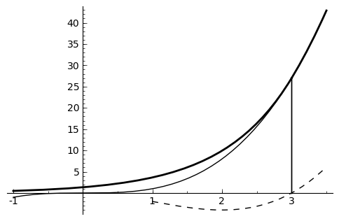
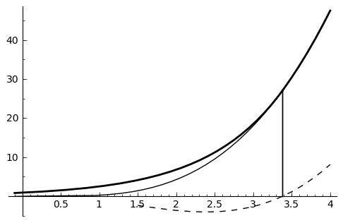
An example for Brownian motion with $r=1/2$ and polynomial with positive $b$ and negative $a$ is shown in Fig. 2. We put in this case

p_{3}(x)=x^{3}-(9/8)x^{2}+3/8,\qquad P_{3}(x)=x^{3}-\frac{33}{8}\,x^{2}+\frac{21}{8}\,x-\frac{3}{8},

and the largest root is $x^{*}=3.3815$ .

4.3 Example 3: Kou’s process for a quartic polynomial

A diffusion process $\{X_{t}\}$ with two sided exponential jumps, defined by the formula

X_{t}=at+\sigma W_{t}+\sum_{k=1}^{N_{t}}Y_{k}-\sum_{k=1}^{N^{\prime}_{t}}Y^{\prime}_{k},

is known in the financial literature as a Kou’s process (see Kou (2002) and Cont and Tankov (2004)). Here $\{N_{t}\}$ (resp. $\{N^{\prime}_{t}\}$ ) is a Poisson process with parameter $\mu$ (resp. $\nu$ ) and $\{Y_{k}\}$ (resp $\{Y^{\prime}_{k}\}$ ) is a sequence of independent exponential random variables with parameter $\alpha$ (resp $\beta$ ). The charactristic exponent (1) of the process is given by

\psi(z)=az+\frac{1}{2}\sigma^{2}z^{2}+\mu\frac{z}{\alpha-z}-\nu\frac{z}{z+\beta},

and the density of the maximum $M$ in this case is a mixture of two exponentials

f_{M}(x)=A_{1}r_{1}e^{-r_{1}x}+A_{2}r_{2}e^{-r_{2}x},

with coefficients

A_{1}={1-r_{1}/\beta\over 1-r_{1}/r_{2}},\quad A_{2}={1-r_{2}/\beta\over 1-r_{2}/r_{1}},

where $0<r_{1}<r_{2}$ are the positive roots of the equation $\psi(z)=r$ (see Mordecki (2003)). In consequence the moments are given by

\mu_{k}=k!\left(\frac{A_{1}}{r_{1}^{k}}+\frac{A_{2}}{r_{2}^{k}}\right).

We consider a quartic polynomial

p(x)=x^{4}+a_{3}x^{3}+a_{2}x^{2}+a_{1}x.

If we denote $P(x)=x^{4}+b_{3}x^{3}+b_{2}x^{2}+b_{1}x+b_{0}$ , applying (16) we obtain

	$\displaystyle b_{3}$	$\displaystyle=a_{3}-4\mu_{1}$
	$\displaystyle b_{2}$	$\displaystyle=a_{2}-6\mu_{2}-3b_{3}\mu_{1}$
	$\displaystyle b_{1}$	$\displaystyle=a_{1}-4\mu_{3}-3b_{3}\mu_{2}-2b_{2}\mu_{1}$
	$\displaystyle b_{0}$	$\displaystyle=-(\mu_{4}+b_{3}\mu_{3}+b_{2}\mu_{2}+b_{1}\mu_{1})$

Assuming that there exists a value $x^{*}$ that satisfies the conditions of Theorem 2, we write the possible value function

V(x)={\operatorname{\mathbf{E}}_{x}}P(x+M)\mathbf{1}_{\{x+M\geq x^{*}\}}=B_{1}e^{r_{1}(x-x^{*})}+B_{2}e^{r_{2}(x-x^{*})},

where

B_{1}=A_{1}r_{1}\int_{0}^{\infty}P(z+x^{*})e^{-r_{1}z}dz,\quad B_{2}=A_{2}r_{2}\int_{0}^{\infty}P(z+x^{*})e^{-r_{2}z}dz.

To proceed we choose values for the parameters:

a=2,\ \sigma=1,\ \mu=1,\ \nu=1,\ \alpha=2,\ \beta=2,\ r=6.

and choose the polynomial

p(x)=x(x-1)(x-2)(x-3)=x^{4}-6x^{3}+11x^{2}-6x.

We obtain $r_{1}=1.4327$ , $r_{2}=2.8740$ , giving $A_{1}=0.5656,$ $A_{2}=0.4344$ . In consequence $x^{*}=4.3706$ . For this sets of parameters the conditions of Theorem 2 are fulfilled (see Figure 3).

References

Alili and Kyprianou (2005) L. Alili, and A.E. Kyprianou, Some remarks on first passage of Lévy processes, the American put and pasting principles, Annals of Applied Probability, 15 (2005), pp. 2062–2080.
Bertoin (1996) J. Bertoin, Lévy processes, Cambridge: Cambridge Univ. Press., 1996.
Boyarchenko and Levendorskiĭ (2002) S. I. Boyarchenko and S.Z. Levendorskiĭ, Perpetual American options under Lévy processes, SIAM Journal on Control and Optimization, 40 (2002), pp. 1663–1696.
Boyarchenko and Levendorskiĭ (2002a) S. I. Boyarchenko and S.Z. Levendorskiĭ, Non-Gaussian Merton-Black-Scholes theory, World Scientific: Singapore, 2002.
Christensen et al. (2013) S. Christensen, P. Salminen and Bao Quoc Ta, Optimal stopping of strong Markov processes, Stochastic Process. Appl. 123 (2013), pp. 1138–1159.
Cont and Tankov (2004) R. Cont and P. Tankov, Financial modelling with jump processes, Boca Raton, FL: Chapman and Hall/CRC 2004.
Darling, Liggett and Taylor (1972) D.A. Darling, T. Liggett and H.M. Taylor, Optimal stopping for partial sums, The Annals of Mathematical Statistics 43 (1972), pp. 1363–1368.
Kou (2002) S. G. Kou, A jump diffusion model for option pricing, Management Science, 48 (2002), pp. 1086–1101.
Kyprianou (2006) A. E. Kyprianou, Introductory lectures on fluctuations of Lévy processes with applications, Springer, Berlin Heidelberg, 2006.
Kyprianou and Surya (2005) A. Kyprianou and B.A. Surya, On the Novikov-Shiryaev Optimal Stopping problems in continous time, Electronic Communications in Probability, 10 (2005), pp. 146–154
Mishura and Tomashyk (2011) Yu. S. Mishura and V.V. Tomashyk, An optimal stopping problem for random walks with polynomial reward functions (Ukrainian) Teor. Imovir. Mat. Stat., 86 (2011), pp. 138–149, translation in Theory Probab. Math. Statist., 86 (2013), pp. 155–167.
Mordecki (2002a) E. Mordecki, Optimal stopping and perpetual options for Lévy processes, Finance and Stochastics, 6 (2002) pp. 473–493.
Mordecki (2002b) E. Mordecki, Perpetual options for Lévy processes in the Bachelier model, Proceedings of the Steklov Mathematical Institute, 237 (2002), pp. 256–264.
Mordecki (2003) E. Mordecki, Ruin probabilities for Lévy processes with mixed-exponential negative jumps, Theory Probab. Appl. , 48 (2003), pp 170–176.
Mordecki and Salminen (2007) E. Mordecki and P. Salminen, Optimal stopping of Hunt and Lévy processes, Stochastics 79 (2007), pp. 233–251.
Novikov and Shiryaev (2004) A. Novikov, and A.N. Shiryaev, On an effective solution of the optimal stopping problem for random walks, Theory of Probability and Their Applications, 49 (2004) pp. 373–382.
Novikov and Shiryaev (2007) A. Novikov, and A.N. Shiryaev, On a solution of the optimal stopping problem for processes with independent increments Stochastics. 79 (2007), pp. 393–406.
Salminen (1985) P. Salminen, P. Optimal stopping of one-dimensional diffusions, Math. Nachr. 124 (1985) pp. 85–101.
Salminen (2007) P. Salminen, Optimal stopping, Appell polynomials, and Wiener-Hopf factorization. Stochastics. 83 (2011), pp. 611–622.
Shiryaev (2008) A.N. Shiryaev, Optimal stopping rules, Springer, Berlin, 2008.
Skorokhod (1991) A. V. Skorokhod, Sluchaĭnye protsessy s nezavisimymi prirashcheniyami, (Russian) 2nd. edition, Nauka, Moscow, 1986. (see also Skorokhod, A. V. Random processes with independent increments Kluwer Academic Publishers, Dordrecht, 1991.
Surya (2007) B.A. Surya, An approach for solving perpetual optimal stopping problems driven by Lévy processes, Stochastics, 79 (2007), pp. 337–361.
Surya (2007a) B. A. Surya, Optimal stopping problems driven by Lévy processes and pasting principles, PhD thesis, 2007.

Optimal stopping for Lévy processes with polynomial rewards

Abstract

1 Introduction

2 Formulation of the problem and main results

Theorem 1.

Remark 1.

Lemma 1.

Proof.

Remark 2.

Lemma 2.

Proof.

Proof of the Theorem 1.

Remark 3.

Remark 4.

Corollary 1 (Surya (2007a)).

Proof of the Corollary.

3 Polynomial rewards

3.1 The averaging polynomial

Remark 5.

Proposition 1.

Proof.

Theorem 2.

Proof.

4 Examples

4.1 Example 1: Quadratic polynomials

4.2 Example 2: Cubic polynomials

4.3 Example 3: Kou’s process for a quartic polynomial

References

Optimal stopping for Lévy processes
with polynomial rewards