Fast Desynchronization For Decentralized Multichannel Medium Access Control

Nikos Deligiannis João F. C. Mota George Smart Yiannis Andreopoulos ^†^†thanks: This work has been presented in part at the 14th International Conference on Information Processing in Sensor Networks (IPSN ’15) [1].^†^†thanks: N. Deligiannis is with the Department of Electronics and Informatics, Vrije Universiteit Brussel, Pleinlaan 2, 1050 Brussels, Belgium, and also with iMinds, Ghent 9050, Belgium (email: ndeligia@etro.vub.ac.be).^†^†thanks: J. F. C. Mota, G. Smart, and Y. Andreopoulos are with the Electronic and Electrical Engineering Department, University College London, Roberts Building, Torrington Place, London, WC1E 7JE, UK (e-mail: {j.mota, george.smart, i.andreopoulos}@ucl.ac.uk).

Abstract

Distributed desynchronization algorithms are key to wireless sensor networks as they allow for medium access control in a decentralized manner. In this paper, we view desynchronization primitives as iterative methods that solve optimization problems. In particular, by formalizing a well established desynchronization algorithm as a gradient descent method, we establish novel upper bounds on the number of iterations required to reach convergence. Moreover, by using Nesterov’s accelerated gradient method, we propose a novel desynchronization primitive that provides for faster convergence to the steady state. Importantly, we propose a novel algorithm that leads to decentralized time-synchronous multichannel TDMA coordination by formulating this task as an optimization problem. Our simulations and experiments on a densely-connected IEEE 802.15.4-based wireless sensor network demonstrate that our scheme provides for faster convergence to the steady state, robustness to hidden nodes, higher network throughput and comparable power dissipation with respect to the recently standardized IEEE 802.15.4e-2012 time-synchronized channel hopping (TSCH) scheme.

Index Terms:

Medium access control, desynchronization, gradient methods, decentralized multichannel coordination.

I Introduction

In wireless sensor networks (WSNs), achieving and maintaining (de)synchronization among the nodes supports various functionalities, including data aggregation, duty cycling, and cooperative communications. In particular, devising protocols that perform desynchronization at the medium access control (MAC) layer is key in achieving fair TDMA scheduling among the nodes in a channel [2, 3, 4, 5, 6, 7].

In order to extend fair TDMA scheduling to large-scale networks, protocols that achieve (de)synchronization across multiple channels [4, 5] are required. Typical approaches are infrastructure-based (i.e., centralized), as they use a coordination channel and/or node and a global clock (e.g., via a GPS system) [5]. Channel hopping is been accepted as a good solution for MAC-layer coordination for dense WSN topologies. According to channel hopping, nodes hop between the available channels of the physical layer such that they are not constantly using a channel with excessive interference. Forming the state-of-the-art, the time-synchronized channel hopping (TSCH) [5] protocol is now part of the IEEE 802.15.4e-2012 standard [8]. In TSCH, each node reserves timeslots within the predefined slotframe interval and within the 16 channels of IEEE 802.15.4. However, filling up the available slots follows an advertising request-and-acknowledgment (RQ/ACK) process on a coordination channel. This channel is prone to interference and self-inflicted collisions when nodes advertise slots aggressively. Moreover, when nodes leave the network, their slots may remain unoccupied for long periods until another advertisement process reassigns them to other nodes. This limits the bandwidth usage per channel and does not allow for fast convergence to the steady state¹¹ 1 Both high network throughput and quick convergence are important for WSNs that operate with a periodic wake-up cycle (or are event-triggered) and must quickly converge to a steady operational state and transmit high data volumes before being re-suspended.. It is also important to note that TSCH requires a coordinator to maintain global time synchronization [3, 5].

To achieve infrastructure-less (i.e., decentralized) WSN MAC-layer coordination, distributed (de)synchro-nization algorithms have attracted a lot of interest [5, 9, 10, 6, 11, 12, 13, 14, 15, 2, 16, 17]. These algorithms are inspired by biological agents modeled as pulse-coupled oscillators (PCOs) [18, 6, 14], namely, as timing mechanisms following a periodic pulsing (i.e., beacon packet transmission at the MAC) that is updated via the timings of pulses heard from other nodes.

§Most work on distributed (de)synchronization is based on the PCO dynamics model introduced by Mirollo and Strogatz [18], and derives several algorithms with properties of practical relevance to WSN deployments, namely: (i) limited listening [19, 2, 20], a property that is imperative for low energy consumption in wireless transceivers; (ii) solutions amenable to multi-hop network topologies and the existence of hidden nodes [11, 17, 2]; (iii) solutions scalable to large groups of nodes [15, 6]; and (iv) modifications that lead to fast convergence to steady state [14, 13, 12, 21]. PCO-based synchronization methods have also been interpreted as consensus algorithms for multi-agent systems [22, 23, 24]. The work in [22] studied synchronization of networked oscillators under heterogeneous time-delays and varying topologies. In [24], the synchronization of networked oscillators was modeled using coupled discrete-time phase locked loops.

Regarding the study of the convergence speed of desynchronization algorithms, mostly estimates based on simulations or empirical measurements have been derived. In effect, only lower bounds [14, 19], order-of-convergence estimates [19, 6, 2] and operational estimates [25] have been established. However, no upper bounds are currently known for the convergence speed of desynchronization algorithms, despite the fact that such bounds provide for worst-case guarantees of time and energy consumption to achieve the state of desynchrony. Furthermore, despite the plethora of works on PCOs, the problem of extending distributed (de)synchronization algorithms to the multichannel case (which is key in today’s wireless networks) has received limited attention. A preliminary attempt was done in [7], where desynchronization was independently applied per channel. The limitation of the scheme in [7] is that, since the nodes in different channels are not synchronized, when a node switches channels convergence needs to be established anew.

In this work, we view the problem of desynchronization as an optimization problem. In particular, we show that a minor modification of the well established Desync algorithm [2, 10] is the gradient descent method applied to a specific optimization problem. Although desynchronization can also be viewed from a consensus perspective [23], the optimization approach is more powerful as it allows deriving faster algorithms [26, 27]. Our contributions are as follows:

•

We establish novel upper bounds on the convergence rate of the Desync process. Such bounds can yield reliable estimates of worst-case energy consumption and time required for convergence, which are important for systems that operate under delay and/or energy constraints.
•

We propose a novel desynchronization algorithm based on Nesterov’s accelerated gradient method [28, 29]. We show, both theoretically and experimentally, that the proposed algorithm leads to faster convergence to steady state than the conventional Desync algorithm [2, 10].
•

We propose a novel distributed multichannel method that jointly performs synchronization across channels and desynchronization within each channel. Contrary to [7], the proposed algorithm leads to time-synchronous multichannel TDMA coordination (where nodes allocated the same timeslot in adjacent channels are synchronized). In this way, nodes can swap channels (thus, avoiding persistent interference in certain channels and achieving higher connectivity) without the network exiting the steady state.
•

Finally, via simulations and experiments using a real WSN deployment abiding by the IEEE802.15.4 standard, we show that our approach leads to decentralized time-synchronous multichannel MAC-layer coordination that achieves higher network throughput compared to the state-of-the-art TSCH [5] protocol, while incurring comparable power consumption.

3.8,4.2) nput270zero $0$ 2)0.630330 nput-12x1 $\theta_{i+1}(t_{i-1})$ nput90x1 $\theta_{i-1}(t_{i-1})$ nput56x3k $\theta_{i}(t_{i-1})$ nput30x3n $\theta_{i}^{\prime}(t_{i-1})$ ncarc-x3kx3n

Fig. 1: Phase update of node

i

according to the Desync algorithm: node

i-1

fires at time

t_{i-1}

, and node

i

updates its phase from

\theta_{i}(t_{i-1})

\theta_{i}^{\prime}(t_{i-1})

, towards the average of the phases of nodes

i-1

and

i+1

, its phase neighbors.

The paper continuous as follows: Section II presents the background on PCO methods, while Section III derives our upper bound for the desynchronization process and proposes our novel accelerated desynchronization algorithm. Section IV presents our novel formulation of multichannel coordination. Simulations and experiments using a WSN deployment are given in Section V, while Section VI concludes the paper.

II Background on Pulse-Coupled Oscillators

Consider a fully-connected WSN comprising $n$ nodes, each acting as a pulse-coupled oscillator [18]. When a node does not interact with others, it broadcasts a fire message or pulse periodically. This is modeled by assigning to node $i$ a phase $\theta_{i}(t)$ , whose value at time $t$ is given by [2, 19]

\theta_{i}(t)=\frac{t}{T}+\phi_{i}\mod{1}\,,

(1)

where $\phi_{i}\in[0,1]$ is the phase offset of node $i$ and $\mod{1}$ denotes the modulo operation with respect to unity. Fig. 1 illustrates (1) graphically: the phase $\theta_{i}(t)$ of node $i$ can be seen as a bead moving clockwise on a circle, whose origin coincides both with $0$ and $1$ [18, 30, 19, 6]. If $\phi_{i}$ is constant, which happens when the nodes do not interact, node $i$ broadcasts a fire message every $T$ time units, when $\theta_{i}(t)=1$ , and then sets its phase to zero. When the nodes interact, e.g., by listening to each others’ messages, they modify their phases (specifically, their phase offsets), according to an update equation that expresses the PCO dynamics [18]. One of the most prominent PCO algorithms for desynchronization at the MAC layer of WSNs is the Desync algorithm [10, 2]. In Desync, the nodes are ordered according to their initial phases: $0\leq\theta_{1}(0)<\theta_{2}(0)<\cdots<\theta_{n}(0)<1$ . Assuming perfect beacon transmission and reception, the order of the firings in Desync will remain the same [10, 2]. The phase $\theta_{i}$ of each node $i$ is updated based on the phases $\theta_{i-1}$ and $\theta_{i+1}$ of its phase neighbors, nodes $i-1$ and $i+1$ , respectively. This is illustrated in Fig. 1: immediately after node $i-1$ transmits a fire message, node $i$ modifies its phase according to

\theta_{i}^{\prime}(t_{i-1})=(1-\alpha)\theta_{i}(t_{i-1})+\alpha\frac{\theta_{i-1}(t_{i-1})+\theta_{i+1}(t_{i-1})}{2}\,,

(2)

where $t_{i-1}$ is the time instant in which node $i-1$ fires, i.e., $\theta_{i-1}(t_{i-1})=1$ , and $i=1,2,\dots,n$ , with periodic extension at the boundaries. The jump-phase parameter $\alpha\in(0,1)$ controls the phase increment [10, 2].

When node $i$ updates its phase, it has stale knowledge of the phase of node $i+1$ , namely, it only knows the previous value of $\theta_{i+1}$ and not the current one. This is because node $i+1$ modified its phase when node $i$ fired, but the value of the new phase has not been “announced” yet [10]. In Desync, each node: (i) updates its phase once in each firing round (we say that a firing round is completed when each node in the network has fired exactly once); (ii) does not need to know the total number of nodes, $n$ , in the network; (iii) requires limited listening, as only the messages from the two phase neighbors are required. These features make Desync quite popular [10, 2]. For a fully-connected network, it has been shown that (2) converges to the state of desynchrony at time $\overline{t}$ , after which the interval between consecutive firings is $T/n$ up to a small threshold $\epsilon$ . Under partial connectivity or hidden nodes, convergence is still achieved under a wide variety of topologies, but the node firings may not be equidistant [2]. It has been conjectured via simulations [30, 10] that Desync converges to desynchrony (i.e., perfect TDMA scheduling) in

r_{\textsc{Desync}}=O\left(\frac{1}{\alpha}n^{2}\ln\frac{1}{\epsilon}\right)

(3)

firing rounds. Recently, under the assumption of uniformly distributed initial firing phases, an operational estimate for the number of firing rounds for the Desync algorithm’s convergence was derived [25]. However, no upper bounds are known for the desynchronization process.

4.0,4.2) nput270zero $0$ 2)0.630330 nput100x1 $\theta_{4}^{(0)}$ nput155x1 $\theta_{3}^{(0)}$ nput185x1 $\theta_{2}^{(0)}$ nput235x1 $\theta_{1}^{(0)}$

3.8,4.2) nput270zero $0$ 2)0.630330 nput5x1 $\theta_{4}^{(0)}$ nput90x1 $\theta_{2}^{(0)}$ nput140x1 $\theta_{1}^{(0)}$ nput60x3k $\theta_{3}^{(0)}$ nput30x3n $\theta_{3}^{(1)}$ ncarc-x3kx3n

4.5,4.2) nput270zero $0$ 2)0.630330 nput275x1 $\theta_{4}^{(0)}$ nput340x1 $\theta_{3}^{(1)}$ nput90x1 $\theta_{1}^{(0)}$ nput40x2k $\theta_{2}^{(0)}$ nput15x2n $\theta_{2}^{(1)}$ ncarc-x2kx2n

3.7,4.2) nput270zero $0$ 2)0.630330 nput90x1 $\theta_{4}^{(0)}$ nput155x1 $\theta_{3}^{(1)}$ nput190x1 $\theta_{2}^{(1)}$ nput265x1k $\theta_{1}^{(0)}$ nput340x1n $\theta_{1}^{(1)}$ ncarc-x1kx1n

4.0,4.2) nput270zero $0$ 2)0.630330 nput25x1 $\theta_{4}^{(0)}$ nput90x1 $\theta_{3}^{(1)}$ nput146x1 $\theta_{3}^{(0)}$ nput125x1 $\theta_{2}^{(1)}$ nput275x1 $\theta_{1}^{(1)}$ nput25x4k $\theta_{4}^{(0)}$ nput350x4n $\theta_{4}^{(1)}$ ncarc-x4kx4n

Fig. 2: Updates during the first iteration of Desync in a

4

-node network: (a) initial phases; no firing has occurred yet; (b) the first update occurs when node

2

fires and after nodes

4

and

3

have fired. The firing of node

2

causes node

3

to update

\theta_{3}^{(0)}

\theta_{3}^{(1)}

. In the remaining steps, node

i

fires and node

j

updates its phase, where

(i,j)

(1,2)

in (c),

(4,1)

in (d), and

(3,4)

in (e). All phases are updated as a function of the initial values, i.e., although some of the phases have already changed, the updates use always

\theta_{1}^{(0)}

\theta_{2}^{(0)}

\theta_{3}^{(0)}

, or

\theta_{4}^{(0)}

, and not the new values.

III Desync as a Gradient Method

We start by showing that, considering a fully-connected network, a minor modification of Desync [2, 10] can be viewed as a gradient descent method solving an optimization problem. Then, we establish novel convergence properties of the resulting method and derive a new accelerated desynchronization primitive.

Staleness of Desync: Fig. 2 shows five consecutive configurations of the phases of the nodes of a network with four nodes. The purpose is to illustrate how the phases of the nodes are updated in the first iteration of Desync [2, 10] and to highlight our minor modification. For simplicity, we omit the time dependence of the phases, but use a superscript to indicate how many times they have been updated. In Fig. 2, no firing has yet occurred. The first update occurs when node $2$ fires, whereby node $3$ updates its phase from $\theta_{3}^{(0)}$ to $\theta_{3}^{(1)}$ [see Fig. 2]. According to (2), this update requires knowing $\theta_{2}$ (which is equal to $1$ because node $2$ is firing) and $\theta_{4}$ (which is known because node $4$ was the first to fire). The second phase update occurs in Fig. 2: node $1$ fires, and node $2$ updates its phase from $\theta_{2}^{(0)}$ to $\theta_{2}^{(1)}$ . According to (2), this update requires the value of $\theta_{1}$ (known because node $1$ is firing) and $\theta_{3}$ . The current value of $\theta_{3}$ (actually, $\theta_{3}^{(1)}$ ) is not known because node $3$ has not fired since it updated its phase. Therefore, node $2$ will use $\theta_{3}^{(0)}$ rather than $\theta_{3}^{(1)}$ . This is why we say that Desync is stale: each update uses stale versions of the phases. In step (d), node $1$ updates its phase and also uses a stale version of the phase of node $2$ . Finally, in step (e), node $4$ updates its phase using a stale version of the phase of node $1$ . We assume, however, that in contrast with the other nodes, this update uses the value $\theta_{3}^{(0)}$ (in gray) and not $\theta_{3}^{(1)}$ .

Assumption 1.

In Desync, node $n$ updates its phase at iteration $k$ using $\theta_{n-1}^{(k-1)}$ in place of $\theta_{n-1}^{(k)}$ .

Via Assumption 1, all updates in Fig. 2 use the initial values $\theta_{1}^{(0)}$ , $\theta_{2}^{(0)}$ , $\theta_{3}^{(0)}$ , and $\theta_{4}^{(0)}$ . In practice, this assumption does not lead to a discernible difference in the performance of Desync.

Vector notation: Suppose we are in the $k$ -th firing round, i.e., all nodes have updated their phases $k-1$ times. We have already mentioned how the firing of a node $i$ , say at time $t_{i}$ , enables other nodes to determine the current value of $\phi_{i}^{(k-1)}$ in (1): $\phi^{(k-1)}_{i}=1-t_{i}/T$ . Knowing this, each node can determine the value of $\theta_{i}^{(k-1)}(t)$ for any time instant. We will now see how the update rule (2) translates into the updates of the phase offsets. Replacing (1) into (2) at firing round (iteration) $k$ , we obtain

	$\displaystyle\theta_{i}^{\prime}(t_{i-1})$	$\displaystyle=\frac{t_{i-1}}{T}+\phi_{i}^{(k)}$
		$\displaystyle=(1-\alpha)\Big[\frac{t_{i-1}}{T}+\phi_{i}^{(k-1)}\Big]$
		$\displaystyle\qquad+\frac{\alpha}{2}\Big[\frac{t_{i-1}}{T}+\phi_{i-1}^{(k-1)}+\frac{t_{i-1}}{T}+\phi_{i+1}^{(k-1)}\Big]$
		$\displaystyle=\frac{t_{i-1}}{T}+(1-\alpha)\phi_{i}^{(k-1)}+\alpha\frac{\phi_{i-1}^{(k-1)}+\phi_{i+1}^{(k-1)}}{2}\,.$

Eliminating the term $t_{i-1}/T$ , we get: $\phi_{i}^{(k)}=(1-\alpha)\phi_{i}^{(k-1)}+\alpha\frac{\phi_{i-1}^{(k-1)}+\phi_{i+1}^{(k-1)}}{2}\,.$ In a strict sense, this expression is only valid for $i=2,\ldots,n-1$ as the updates for nodes $1$ and $n$ require a correcting term to compensate the fact that each $\theta$ wraps around $1$ . Therefore, the updates for all nodes are

$\displaystyle\phi_{1}^{(k)}$	$\displaystyle=(1-\alpha)\phi_{1}^{(k-1)}+\frac{\alpha}{2}\big(\phi_{2}^{(k-1)}+\phi_{n}^{(k-1)}-1\big)$	(4)
$\displaystyle\phi_{i}^{(k)}$	$\displaystyle=(1-\alpha)\phi_{i}^{(k-1)}+\frac{\alpha}{2}\big(\phi_{i-1}^{(k-1)}+\phi_{i+1}^{(k-1)}\big)\,,\,2\leq i\leq n-1$	(5)
$\displaystyle\phi_{n}^{(k)}$	$\displaystyle=(1-\alpha)\phi_{n}^{(k-1)}+\frac{\alpha}{2}\big(\phi_{n-1}^{(k-1)}+\phi_{1}^{(k-1)}+1\big)\,.$	(6)

Without Assumption 1, $\phi_{1}^{(k-1)}$ in (6) would be replaced with $\phi_{1}^{(k)}$ . It is, however, this assumption that enables us to write (4)-(6) in vector form:

\boldsymbol{\phi}^{(k)}=\begin{bmatrix}1-\alpha&\frac{\alpha}{2}&0&\cdots&0&\frac{\alpha}{2}\\ \frac{\alpha}{2}&1-\alpha&\frac{\alpha}{2}&\cdots&0&0\\ \vdots&&\ddots&&\vdots&\vdots\\ \frac{\alpha}{2}&0&0&\cdots&\frac{\alpha}{2}&1-\alpha\end{bmatrix}\boldsymbol{\phi}^{(k-1)}\\ -\frac{\alpha}{2}\boldsymbol{d}\,,

(7)

where $\boldsymbol{\phi}^{(k)}=(\phi_{1}^{(k)},\phi_{2}^{(k)},\ldots,\phi_{n}^{(k)})\in\mathbb{R}^{n}$ is a vector containing the phases of all the nodes at iteration $k$ , and $\boldsymbol{d}:=(1,0,\ldots,0,-1)\in\mathbb{R}^{n}$ . Equation (7) has the format of the updates usually found in the discrete-time consensus literature [31, 32, 23] . In particular, the matrix in (7) can be seen as the Perron matrix of a network with a ring topology and the vector $\boldsymbol{d}$ can be seen as an input bias [23]. This observation can be used to provide upper bounds on the convergence rate of (7). However, one can view (7) as an algorithm solving an optimization problem since, besides also providing upper bounds, this interpretation enables the derivation of an accelerated version of desynchronization. This interpretation is formalized next.

Proposition 1.

Let $\boldsymbol{\phi}^{(k)}=(\phi_{1}^{(k)},\phi_{2}^{(k)},\dots,\phi_{n}^{(k)})$ denote the phases of all nodes at firing round $k$ . If Assumption 1 holds, then Desync (2) and (7) is the steepest descent method applied to

\underset{\boldsymbol{\phi}}{\text{\emph{minimize}}}\,\,\,\,g(\boldsymbol{\phi}):=\frac{1}{2}\big\|\boldsymbol{D}\boldsymbol{\phi}-v\boldsymbol{1}_{n}+\boldsymbol{e}_{n}\big\|_{2}^{2}

(8)

where $v=1/n$ , $\boldsymbol{1}_{n}\in\mathbb{R}^{n}$ is the vector of ones, $\boldsymbol{e}_{n}=(0,0,\ldots,0,1)\in\mathbb{R}^{n}$ , and

\boldsymbol{D}=\begin{bmatrix}-1&1&0&0&\dots&0\\ 0&-1&1&0&\dots&0\\ \vdots&\ddots&&\ddots&&\vdots\\ 0&\dots&0&0&-1&1\\ 1&\dots&0&0&0&-1\\ \end{bmatrix}\in\mathbb{R}^{n\times n}\,.

(9)

Specifically, the updates in (7) can be written as

\boldsymbol{\phi}^{(k)}=\boldsymbol{\phi}^{(k-1)}-\frac{\alpha}{2}\nabla g(\boldsymbol{\phi}^{(k-1)})\,.

(10)

Proof:

Since $\boldsymbol{D}^{T}\boldsymbol{1}_{n}=\boldsymbol{0}_{n}$ , we have

\nabla g\left(\boldsymbol{\phi}\right)=\boldsymbol{D}^{T}(\boldsymbol{D}\boldsymbol{\phi}-v\boldsymbol{1}_{n}+\boldsymbol{e}_{n})=\boldsymbol{D}^{T}\boldsymbol{D}\boldsymbol{\phi}+\boldsymbol{d}\,,

(11)

where $\boldsymbol{d}=\boldsymbol{D}^{T}\boldsymbol{e}_{n}$ is the vector that appears in (7). Therefore, the steepest descent applied to (8) yields

$\displaystyle\boldsymbol{\phi}^{(k)}$	$\displaystyle=\boldsymbol{\phi}^{(k-1)}-\beta\nabla g(\boldsymbol{\phi}^{(k-1)})$
	$\displaystyle=\boldsymbol{\phi}^{(k-1)}-\beta\boldsymbol{D}^{T}\boldsymbol{D}\boldsymbol{\phi}^{(k-1)}-\beta\boldsymbol{d}$
	$\displaystyle=(\boldsymbol{I}_{n}-\beta\boldsymbol{D}^{T}\boldsymbol{D})\boldsymbol{\phi}^{(k-1)}-\beta\boldsymbol{d}\,,$	(12)

where $\boldsymbol{I}_{n}$ is the identity matrix in $\mathbb{R}^{n}$ . Replacing $\beta=\alpha/2$ , we obtain

\boldsymbol{\phi}^{(k)}=(\boldsymbol{I}_{n}-\frac{\alpha}{2}\boldsymbol{D}^{T}\boldsymbol{D})\boldsymbol{\phi}^{(k-1)}-\frac{\alpha}{2}\boldsymbol{d}\,,

(13)

The last equation is exactly (7). ∎

We set $v=\frac{1}{n}$ in (8) to emphasize that the goal of Desync is to disperse the $n$ phases throughout $[0,1]$ . However, any other value for $v$ would lead to the same update rule, since the gradient of the objective function does not depend on $v$ ; see (11) in the proof. This confirms the fact that Desync does not require the knowledge of the number of nodes, $n$ , in the network [10]. Notice also that $\boldsymbol{D}$ is not full rank; therefore, the objective of (8) is not strictly convex. Indeed, the nullspace of $\boldsymbol{D}$ is $\{z\,\boldsymbol{1}_{n}\,:\,z\in\mathbb{R}\}\cup\{\boldsymbol{0}_{n}\}$ . Consequently, if $\overline{\boldsymbol{\phi}}$ is a solution of (8), so is $\overline{\boldsymbol{\phi}}+z\,\boldsymbol{1}_{n}$ for any $z\in\mathbb{R}$ . We notice that the interpretation of Proposition 1 is akin to the one that views consensus algorithms as gradient descent methods for minimizing $\sum_{i=1}^{n}(\phi_{i}-\theta_{i})^{2}$ , where $\theta_{i}$ is the observation of agent $i$ [33, 26].

This interpretation of Desync provides for: (i) an alternative way to establish the values of $\alpha$ for which convergence holds, and (ii) an upper bound on the number of the firing rounds until convergence.

Corollary 1.

Every limit point of the sequence produced by the Desync algorithm (7) with $\alpha\in(0,1)$ is a stationary point of (8).

Proof:

The proof is given in Appendix A. ∎

Corollary 2.

Let $\boldsymbol{\phi}^{(0)}$ represent the vector of initial phases, and let $\boldsymbol{\phi}^{\star}$ be any solution of (8). Suppose $\boldsymbol{0}_{n}\leq\boldsymbol{\phi}^{(0)}\leq\boldsymbol{1}_{n}$ . Then, the number of firing rounds, $r_{\textsc{D}}$ , that Desync (4)–(6) requires in order to generate a point $\overline{\boldsymbol{\phi}}$ that has accuracy $\epsilon:=g\big(\overline{\boldsymbol{\phi}}\big)$ is upper bounded as

	$\displaystyle r_{\textsc{D}}$	$\displaystyle\leq\frac{\\|\boldsymbol{\phi}^{(0)}-\boldsymbol{\phi}^{\star}\\|_{2}^{2}}{2\alpha(1-\alpha)}\bigg(\frac{1}{\epsilon}-\frac{1}{g\big(\boldsymbol{\phi}^{(0)}\big)}\bigg)$		(14)
		$\displaystyle\leq\frac{1}{6n\alpha(1-\alpha)}\left[\frac{7}{2}n^{2}+3n+4\right]\bigg(\frac{1}{\epsilon}-\frac{1}{g\big(\boldsymbol{\phi}^{(0)}\big)}\bigg)\,.$		(15)

Proof:

The proof is given in Appendix A. ∎

Corollary 1 confirms Theorem 1 in [10] regarding the stability and convergence of Desync, albeit using different tools and without requiring simulations to illustrate the avoidance of limit cycles. Corollary 2 complements the existing order-of-convergence estimate of (3) and the operational estimates derived by Buranapanichkit et al. [25] by deriving an upper bound for the firing rounds to achieve convergence. Such an upper bound allows for reliable estimates of worst-case energy consumption and time, expressed in number of firing rounds or iterations, required to reach convergence. These estimates are important for systems that operate under delay and/or energy constraints. Notice that the bound in (15) is a function of known system parameters, namely, the number of nodes $n$ , the jump-phase parameter $\alpha$ , the tolerance parameter $\epsilon$ , and the evaluation of $g(\cdot)$ on the initial phase vector (the latter can be ignored yielding a looser bound).

The Fast-Desync algorithm based on Nesterov: A key advantage of viewing desynchronization as an optimization problem is that we can create new primitives that converge to desynchrony much faster. Particularly, we can use Nesterov’s fast gradient algorithm [29, 28] (here we use the adaptation in [34]):


$\displaystyle\boldsymbol{\phi}^{(k)}$	$\displaystyle=\boldsymbol{\mu}^{(k-1)}-\beta\,\nabla g(\boldsymbol{\mu}^{(k-1)})$	(16a)
$\displaystyle\boldsymbol{\mu}^{(k)}$	$\displaystyle=\boldsymbol{\phi}^{(k)}+\frac{k-1}{k+2}\big(\boldsymbol{\phi}^{(k)}-\boldsymbol{\phi}^{(k-1)}\big)\,,$	(16b)

where $\boldsymbol{\mu}^{(k)}\in\mathbb{R}^{n}$ is an auxiliary vector. Nesterov’s method is applicable under the same assumptions as the steepest descent, i.e., when $g$ is continuously differentiable and its gradient is Lipschitz continuous with constant $L$ . However, it requires $0<\beta\leq 1/L$ rather than $0<\beta<2/L$ . At the expense of small extra memory and computation, Nesterov’s method takes $O(1/\sqrt{\epsilon})$ iterations to produce a point $\overline{\boldsymbol{\phi}}$ that satisfies $g(\overline{\boldsymbol{\phi}})-g(\boldsymbol{\phi}^{\star})\leq\epsilon$ , where $\boldsymbol{\phi}^{\star}$ minimizes $g$ . Recall that the steepest descent takes $O(1/\epsilon)$ to produce such a point [cf. (15)]. We shall show that this improved performance in terms of bounds is also observed experimentally. Note that $\boldsymbol{\mu}^{(k)}$ , $\boldsymbol{\phi}^{(k)}$ converge to the same point, i.e., $\|\boldsymbol{\phi}^{(k)}-\boldsymbol{\mu}^{(k)}\|\rightarrow{0}$ as $k\rightarrow{\infty}$ . More importantly, Nesterov showed in [29] that (16) has optimal convergence rate among first-order methods, i.e., methods that use information about first-order derivatives only, possibly from all past iterations.

We propose applying Nesterov’s algorithm (16a)-(16b) to solve (8). This yields a primitive that we call Fast-Desync. Node $i=1,\ldots,n$ holds two variables $\phi_{i}$ and $\mu_{i}$ , which are updated at iteration $k$ as


$\displaystyle\phi_{i}^{(k)}$	$\displaystyle=(1-\alpha)\mu_{i}^{(k-1)}+\frac{\alpha}{2}\big(\mu_{i-1}^{(k-1)}+\mu_{i+1}^{(k-1)}-d_{i}\big)$	(17a)
$\displaystyle\mu_{i}^{(k)}$	$\displaystyle=\phi_{i}^{(k)}+\frac{k-1}{k+2}\big(\phi_{i}^{(k)}-\phi_{i}^{(k-1)}\big)\,,$	(17b)

where $d_{1}=1$ , $d_{n}=-1$ , and $d_{i}=0$ for $i=2,\ldots,n-1$ . Note that (17a) is identical to the Desync updates (4)–(6). The only detriment is that each node needs an extra memory register to store $\phi_{i}^{(k-1)}$ , which is used in (17b), and perform the extra computations in (17b). Under this modification, the following holds:

Corollary 3.

Let $\alpha\in(0,1/2]$ and let $\boldsymbol{0}_{n}\leq\boldsymbol{\phi}^{(0)}=\boldsymbol{\mu}^{(0)}\leq\boldsymbol{1}_{n}$ represent the vectors of initial phases. Let also $\boldsymbol{\phi}^{\star}$ be any solution of (8). Then, the number of firing rounds that Fast-Desync (17a)-(17b) requires to generate a point $\overline{\boldsymbol{\phi}}$ that has accuracy $\epsilon:=g(\overline{\boldsymbol{\phi}})$ is upper bounded as

	$\displaystyle r_{\textsc{FD}}$	$\displaystyle\leq\frac{2}{\sqrt{\alpha\,\epsilon}}\big\\|\boldsymbol{\phi}^{(0)}-\boldsymbol{\phi}^{\star}\big\\|_{2}$		(18)
		$\displaystyle\leq 2\sqrt{\frac{1}{3n\alpha\epsilon}\left[\frac{7}{2}n^{2}+3n+4\right]}\,.$		(19)

Proof:

The proof is given in Appendix A. ∎Contrasting (15) and (19) we notice that Fast-Desync allows for significant reduction in the order-of-iterations for convergence compared to Desync, particularly, $O(\sqrt{n/\epsilon})$ versus $O(n/\epsilon)$ , respectively.

Refer to caption — Fig. 3: (a) Initial random state of $n=14$ nodes in $C=4$ channels; (b) steady state of the proposed protocol with $n_{c}=3$ nodes for channels $c=1$ and $c=2$ , and $n_{c}=4$ nodes in channels $c=3$ and $c=4$ . The Desync nodes (in white) allow for intra-channel desynchronization, while the Sync nodes (in grey) provide for cross-channel synchronization. Nodes that belong to balanced channel and that fire synchronously can swap channels. The horizontal position of a node indicates the firing moment.

IV Extension To Decentralized Multichannel Coordination

We now describe our algorithm that jointly applies synchronization across channels and desynchronization in each channel. We assume that all nodes can receive all fire message broadcasts in their channel. We will show experimentally, however, that our proposal works even for densely-connected WSNs (when some nodes cannot be reached by others), as Desync still converges in such cases [2]. We first describe our protocol.

IV-A Proposed Decentralized Multichannel MAC-layer Coordination

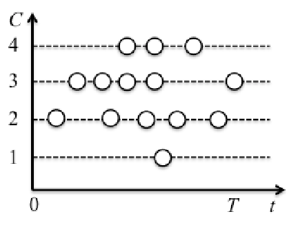
Let a WSN comprise $n$ nodes that are initially randomly distributed in $C$ channels [see Fig. 3(a)]—for example, the $C=16$ channels of the IEEE 802.15.4 standard [35, 36]. The maximum achievable throughput per node is obtained when the nodes are uniformly distributed across the available channels and a perfect TDMA scheduling is reached in each channel. When the total number of nodes in the network, $n$ , is divisible by $C$ our protocol will lead to $n_{c}=\frac{n}{C}$ nodes being present in each channel, alternatively, $n_{c}=\left\{\left\lfloor\frac{n}{C}\right\rfloor,\left\lceil\frac{n}{C}\right\rceil\right\}$ nodes will be present in each channel, as shown in Fig. 3(b).

Existing mechanisms, such as the one in [7], can take place during convergence to balance the number of nodes. Specifically, a node lying in channel $c$ may switch to channel $c+1$ (with cyclic extension at the border), if it detects that less nodes are present there. Detection of the number of nodes in a channel is possible by integrating this information in the fire messages transmitted by the nodes. In [7], in order to detect the number of nodes in channel $c+1$ , nodes within channel $c$ proactively switched channels for short time intervals [7]. Here, however, we follow a different approach, which is akin to the proposed algorithm. In particular, a single node (which we later call Sync) lying in channel $c$ is elected to listen for fire messages in channel $c+1$ . This specific node may jump to the next channel if it detects that less nodes are present there. When a Sync node jumps from one channel to the next, both channels are set to elect their Sync nodes anew. In order to avoid a race condition, where nodes continuously jump channels, the following conditions are defined for channel switching:

\begin{cases}n_{c}-n_{c+1}\geq{1},\mbox{if}\ c\in[1,C)\\ n_{c}-n_{c+1}\geq{2},\mbox{if}\ c=C\end{cases}

where $n_{c}$ denotes the number of nodes present in channel $c$ , with $n=\sum\limits_{c=1}^{C}n_{c}$ . The switching rule and conditions ensure that, after a few firing periods, there will be $n_{c}\in\{\left\lfloor\frac{n}{C}\right\rfloor,\left\lceil\frac{n}{C}\right\rceil\}$ nodes in each channel $c$ .

When the channels have been balanced, the proposed iterative joint synchronization-desynchronization algorithm is applied. By considering that each node acts as a pulse-coupled oscillator with a period of $T$ seconds, our novel algorithm (see Section IV-B) leads to decentralized multichannel round-robin scheduling. The nodes in each channel are divided in two classes. Specifically, all but one node in each channel apply desynchronization so as to achieve TDMA within the channel (these nodes are denoted as “Desync”). Desync nodes operate only within their channel, firing and listening to messages from the other nodes in their channel. In addition, one “Sync” node per channel performs cross-channel synchronization to achieve a time-synchronous slot structure [Fig. 3(b)]. The Sync node of each channel listens for the Sync fire message in the next channel²² 2 We consider a cyclic behavior between channels 1 and 16 of IEEE 802.15.4 [36, 35]. Namely, the Sync node at channel 16 listens for the fire message from the Sync node in channel 1.. A node can be designated as the Sync node in a channel based on a pre-established rule, e.g., the node with the smallest node ID, or the node with the highest battery level (all nodes can be made to report their node ID and battery status in their beacon messages).

We highlight that the existence of a Sync node in each channel calls for an iterative algorithm performed jointly across the available channels (see Section IV-B). This is fundamentally different from prior schemes, e.g., [7], which applied desynchronization in each channel independently. In contrast, cross-channel synchronization allows for a channel swapping mechanism to be applied in the converged state. Specifically, nodes (both of Sync and Desync type) that fire synchronously in adjacent channels can swap channels and time-slots in pairs using a simple RQ/ACK scheme³³ 3 Swap RQ/ACK packets are transmitted at another channel during a short interval after and before a node’s fire message transmission. [see Fig. 3(b)]. Channel swapping allows for communication between nodes initially present in different channels without leaving the steady network state, thereby achieving increased connectivity. Conversely, in [7], when a node changes channels, convergence to TDMA in the channel needs to be established anew.

According to our protocol, starting from any random state, the network reaches a steady state, where: (i) the same number of nodes is present in adjacent channels, (ii) the nodes in each channel have converged to a TDMA scheduling and (iii) the nodes in channels with the same number of nodes have a parallel TDMA scheduling, where nodes allocated with the same time-slot order transmit synchronously [see Fig. 3(b)].

IV-B Proposed Joint Sync-Desync Algorithm

We now describe the proposed joint algorithm that allows for synchronization of Sync nodes across channels and desynchronization of Desync nodes in each channel. Let $\theta_{c,i}$ (resp. $\phi_{c,i}$ ) denote the phase (resp. phase offset) of node $i=1,\dots,n_{c}$ in channel $c=1,\dots,C$ . Without loss of generality and to simplify notation, let the node $i=1$ be the Sync node in each channel⁴⁴ 4 As explained in Section IV-A, any node in a channel can be the Sync node. This convention is only used to simplify our notation.. Desync nodes $i=2,\dots,n_{c}$ in channel $c$ are coupled with phase neighboring nodes (both Desync and Sync) in the same channel. Namely, any Desync node $i$ in channel $c$ updates its phase offset $\phi_{c,i}$ when node $i-1$ in the same channel transmits a fire message, i.e., when $\theta_{c,i-1}=1$ . The Sync node in channel $c$ , in turn, receives coupling only from the Sync node in channel $c+1$ (channel 1 for $c=C$ ). Specifically, it updates its phase offset $\phi_{c,1}$ when the Sync node in the next channel fires, that is, when $\theta_{c+1,1}=1$ . An illustrative example of the phase updates performed by the proposed algorithm is given in Fig. 4.

Problem formulation: Inspired by the interpretation given in Proposition 1, we address the multichannel coordination problem by solving

\underset{\boldsymbol{\phi_{1}},\ldots,\boldsymbol{\phi_{C}}}{\text{minimize}}\,\,\,h(\boldsymbol{\phi_{1}},\ldots,\boldsymbol{\phi_{C}}):=\sum_{c=1}^{C}\frac{1}{2}\big\|\boldsymbol{D_{c}}\boldsymbol{\phi_{c}}-\frac{1}{n_{c}}\boldsymbol{1}_{n_{c}}+\boldsymbol{e_{c}}\big\|_{2}^{2}\\ +\sum_{c=1}^{C}\frac{1}{2}\Big(\boldsymbol{w_{c+1}}^{T}\boldsymbol{\phi}_{c+1}-\boldsymbol{w_{c}}^{T}\boldsymbol{\phi}_{c}\Big)^{2}\,,

(20)

where $\boldsymbol{\phi_{c}}=(\phi_{c,1},\phi_{c,2},\ldots,\phi_{c,n_{c}})\in\mathbb{R}^{n_{c}}$ is the vector containing the phase offsets of all nodes of channel $c$ , $\boldsymbol{D_{c}}\in\mathbb{R}^{n_{c}\times n_{c}}$ is the matrix of (9) with dimensions $n_{c}\times n_{c}$ , $\boldsymbol{e_{c}}=(0,0,\ldots,1)\in\mathbb{R}^{n_{c}}$ and $\boldsymbol{w_{c}}=(1,0,\ldots,0)\in\mathbb{R}^{n_{c}}$ . While the first term of $h$ enforces desynchronization among the nodes of the same channel [note that each summand has the same format as $g$ in (8)], the second term enforces synchronization among the first nodes of each channel. We remark that the second term of (20) is commonly found in the design of optimization-based consensus algorithms [26, 33, 27].

Intuition: We show that the direct application of the gradient descent method to solve (20) leads to updates (for the Sync nodes) that cannot be implemented in a practical WSN. However, the proposed solution will be a modification of those updates.

Taking into account that $\boldsymbol{D_{c}}^{T}\boldsymbol{1}_{n_{c}}=\boldsymbol{0}_{n_{c}}$ for any $c$ , the gradient of $h$ with respect to $\boldsymbol{\phi_{c}}$ is given by

\nabla_{\boldsymbol{\phi_{c}}}h(\boldsymbol{\phi_{1}},\ldots,\boldsymbol{\phi_{C}})=\boldsymbol{D_{c}}^{T}\boldsymbol{D_{c}}\boldsymbol{\phi_{c}}+\boldsymbol{d_{c}}\\ +\Big(2\boldsymbol{w_{c}}^{T}\boldsymbol{\phi_{c}}-\boldsymbol{w_{c-1}}^{T}\boldsymbol{\phi_{c-1}}-\boldsymbol{w_{c+1}}^{T}\boldsymbol{\phi_{c+1}}\Big)\boldsymbol{w_{c}}\,,

(21)

where $\boldsymbol{d_{c}}:=(1,0,\ldots,0,-1)\in\mathbb{R}^{n_{c}}$ . Therefore, the partial derivative of $h$ with respect to $\phi_{c,i}$ is

\frac{\partial}{\partial\,\phi_{c,i}}h(\boldsymbol{\phi_{1}},\ldots,\boldsymbol{\phi_{C}})\\ =\left\{\begin{array}[]{ll}4\phi_{c,i}-\phi_{c,i-1}-\phi_{c,i+1}-\phi_{c-1,i}-\phi_{c+1,i}&,\,\,i=1\\ 2\phi_{c,i}-\phi_{c,i-1}-\phi_{c,i+1}+(\boldsymbol{d_{c}})_{i}&,\,\,i\neq 1\,,\end{array}\right.

where $(\boldsymbol{d_{c}})_{i}$ denotes the $i$ -th component of $\boldsymbol{d_{c}}$ . The gradient descent with stepsize $\beta$ applied to (20) yields for node $i$ of channel $c$ : $\phi_{c,i}^{(k)}=\phi_{c,i}^{(k-1)}-\beta\frac{\partial}{\partial\,\phi_{c,i}}h(\boldsymbol{\phi_{1}}^{(k-1)},\ldots,\boldsymbol{\phi_{C}}^{(k-1)})$ . Replacing $\beta$ with $\alpha/2$ , we obtain

\phi_{c,i}^{(k)}=(1-2\alpha)\phi_{c,i}^{(k-1)}+\frac{\alpha}{2}(\phi_{c,i-1}^{(k-1)}+\phi_{c,i+1}^{(k-1)}+\phi_{c-1,i}^{(k-1)}+\phi_{c+1,i}^{(k-1)})\,,

(22)

for $i=1$ , and

\phi_{c,i}^{(k)}=(1-\alpha)\phi_{c,i}^{(k-1)}+\frac{\alpha}{2}(\phi_{c,i-1}^{(k-1)}+\phi_{c,i+1}^{(k-1)}-(\boldsymbol{d_{c}})_{i})\,,

(23)

for $i\neq 1$ . The update of (23) is similar to the Desync algorithm phase update in (4)–(6). However, the derived update for the Sync node, given in (22), does not abide by the coupling rules mentioned in Section IV-A. Specifically, to implement (22) in a wireless transceiver, each Sync node has to listen for fire messages in its own channel, as well as in the previous and the next channel. This is impractical with the half-duplex transceiver hardware in IEEE 802.15.4-based WSNs. This issue stems from the symmetry of the matrix $\boldsymbol{I}_{n}-\beta\boldsymbol{D}^{T}\boldsymbol{D}$ [cf. (21) and (12)]. To alleviate this issue, we propose modifying directly the matrix associated with the iterations (22) and (23). Our modification is based on the insight that there is one degree of freedom in each channel. Therefore, we can fix the phase of one of the nodes at an arbitrary value. Our approach is to modify (22) and (23) to have the first nodes of each channel performing a simple consensus algorithm [31] (while the remaining nodes perform a Desync algorithm).

Multichannel Sync-Desync (MuCh-Sync-Desync): For simplicity and without loss of generality, we assume that all channels have the same number of nodes: $n:=n_{1}=n_{2}=\cdots=n_{C}$ . The iteration we propose is

\begin{bmatrix}\boldsymbol{\phi_{1}}^{(k)}\\ \boldsymbol{\phi_{2}}^{(k)}\\ \vdots\\ \boldsymbol{\phi_{C}}^{(k)}\end{bmatrix}=\underbrace{\begin{bmatrix}\boldsymbol{Q_{1}}&\boldsymbol{Q_{2}}&\boldsymbol{0}&\cdots&\boldsymbol{0}\\ \boldsymbol{0}&\boldsymbol{Q_{1}}&\boldsymbol{Q_{2}}&\cdots&\boldsymbol{0}\\ \vdots&&\ddots&&\vdots\\ \boldsymbol{0}&\boldsymbol{0}&\cdots&\boldsymbol{Q_{1}}&\boldsymbol{Q_{2}}\\ \boldsymbol{Q_{2}}&\boldsymbol{0}&\boldsymbol{0}&\cdots&\boldsymbol{Q_{1}}\end{bmatrix}}_{=:\boldsymbol{M}}\begin{bmatrix}\boldsymbol{\phi_{1}}^{(k-1)}\\ \boldsymbol{\phi_{2}}^{(k-1)}\\ \vdots\\ \boldsymbol{\phi_{C}}^{(k-1)}\end{bmatrix}\\ +\underbrace{\beta\begin{bmatrix}\boldsymbol{e}_{n}\\ \boldsymbol{e}_{n}\\ \vdots\\ \boldsymbol{e}_{n}\end{bmatrix}}_{=:\boldsymbol{b}}\,,

(24)

where $\boldsymbol{0}$ is the $n\times n$ zero matrix, $\boldsymbol{e}_{n}:=(0,0\ldots,0,1)\in\mathbb{R}^{n}$ , $\boldsymbol{Q_{2}}:=\text{Diag}(\gamma,0,\ldots,0)\in\mathbb{R}^{n\times n}$ , $0<\gamma<1$ , and $\boldsymbol{Q_{1}}$ is the $n\times n$ matrix defined as

\boldsymbol{Q_{1}}:=\begin{bmatrix}1-\gamma&0&0&0&\cdots&0&0\\ \beta&1-2\beta&\beta&0&\cdots&0&0\\ 0&\beta&1-2\beta&\beta&\cdots&0&0\\ \vdots&&&\ddots&&\vdots&\vdots\\ \beta&0&0&0&\cdots&\beta&1-2\beta\end{bmatrix}\,.

In other words, in each channel $c$ , node $i\neq 1$ performs the update (23), while node $1$ performs

\phi_{c,1}^{(k)}=(1-\gamma)\phi_{c,1}^{(k-1)}+\gamma\phi_{c+1,1}^{(k-1)}\,.

(25)

Recall that the phase update of the Sync node in channel $c$ is performed when the Sync node in channel $c+1$ fires, i.e., when $\theta_{c+1,i}(t_{c+1,i})=1$ . Adding $\frac{t_{c+1,i}}{T}$ in both sides of (25) as well as replacing $\phi_{c+1,i}=1-\frac{t_{c+1,i}}{T}$ and using (1) leads to the following phase update for the Sync node in channel $c$ :

\theta_{c,1}^{\prime}(t_{c+1,1})=(1-\gamma)\theta_{c,1}(t_{c+1,1})+\gamma\mod{1}.

(26)

Since $0\leq\theta_{c,1}(t)\leq 1$ , it is straightforward to show that, for $0<\gamma<1$ , (26) provides for inhibitory coupling⁵⁵ 5 Similar to other synchronization algorithms [15], every time the Sync node in channel $c+1$ fires the Sync node in the previous channel will increase its phase towards 1 according to (26). between the Sync nodes in subsequent channels, thereby leading to synchronization of their phases. In the following proposition we establish that the update (24) converges to a solution of the optimization problem (20). In this case, however, we cannot obtain an explicit convergence rate. Note that the matrix $\boldsymbol{M}$ is not symmetric, which complicates the convergence analysis. Note also that, when the number of nodes per channel varies, the sizes of vectors $\boldsymbol{\phi}$ , $\boldsymbol{e}$ , and matrices $\boldsymbol{Q_{1}}$ and $\boldsymbol{Q_{2}}$ in (24) vary per channel $c=1,\dots,C$ , but their format is the same. Moreover, the update equations, described in (23) and (25) remain the same.

Proposition 2.

Let $0<\gamma<1$ and $0<\beta<\frac{1}{2}$ . Then, the sequence produced by (24) converges to a solution of (20).

Proof:

The proof is given in Appendix B. ∎In MuCh-Sync-Desync—formed by (23) and (25)—the Desync and Sync nodes per channel update their phases only once during a firing round in the channel. Similarly to existing (de)synchronization algorithms, the role of the parameters $\alpha$ and $\gamma$ in the updates of (23) and (25) is to compensate for missed fire messages and to not allow their propagation throughout all nodes and channels in the network.

Since the update of the Desync nodes in each channel follows the phase update in (4)–(6), the corresponding Nesterov modification can be applied to speed-up desynchronization in each channel. This approach leads to the Fast-MuCh-Sync-Desync version of our algorithm, of which the convergence speed is assessed in the next section.

V Experimental Evaluations

V-A Simulation Results

All simulations were performed in MATLAB, by extending the event-driven simulator in [2]. Initially, we examine the performance of Desync versus its fast counterpart based on Nesterov’s algorithm. Then, we assess the performance of the proposed MuCh-Sync-Desync algorithm and its fast version. We use two convergence thresholds, i.e., $\epsilon=10^{-3}$ and $\epsilon=10^{-4}$ . Convergence is reported at the firing round where the phases $\overline{\boldsymbol{\phi}}$ of the nodes minimize the objective function in (8) with accuracy $g\left(\overline{\boldsymbol{\phi}}\right)\leq\epsilon$ . Following existing desynchronization schemes [2, 10], our algorithms’ updates are performed on the nodes’ phases $\theta_{i}$ , as Assumption 1 does not need to be followed in practice. This simplifies the implementation, as we do not need to know the order of firings. All simulations were repeated 400 times and average results are reported.

The results of applying desynchronization at a given channel using either Desync [10, 2] or the proposed Fast-Desync algorithm are presented in Fig. 5(a) and (b) for $n=4$ and $n=8$ nodes, respectively. Although our analysis proves that Fast-Desync converges for $\alpha\in(0,0.5]$ , convergence is actually achieved for $\alpha\in(0,1)$ . In fact, Fast-Desync systematically reduces the required number of iterations to convergence (i.e., irrespective of the value of the parameter $\alpha$ ), leading to a 2.6%–28.6% speed-up with respect to Desync. Furthermore, the convergence speed-up increases when a strict threshold ( $\epsilon=10^{-4}$ ) is used. The improvement is more significant at low and medium values of $\alpha$ , which are typically used in practice to attenuate the impact of missed fire messages.

Fig. 6 depicts the maximum number of required firing rounds for convergence of Desync and Fast-Desync versus the bounds in Corollaries 2 and 3. The difference between Desync and Fast-Desync is not visible now due to the logarithmic scale. Because of the low $\epsilon$ value in the denominator of (15) the Desync upper bound appears to be loose. ±However, the Fast-Desync bound in (19) offers a tighter characterization of the simulation-based convergence iterations and follows a trend very similar to the simulation results.

We now evaluate the convergence properties of the proposed MuCh-Sync-Desync and its fast version. The results are given in Fig. 7(a) and (b) for $n_{c}=4$ nodes per channel in $C=6$ and $C=16$ channels, respectively. Contrasting these results with the ones in Fig. 5, we observe that the proposed multichannel algorithm requires approximately only 10–20% more firing rounds to reach convergence than the single-channel Desync algorithm. It is also worth noticing that the proposed Fast-MuCh-Sync-Desync version offers a notable convergence speed-up (i.e., 6.01%–42.54%) with respect to the simple MuCh-Sync-Desync algorithm, irrespective of the number of channels.

V-B Experiments with TelosB Motes

Experimental setup: We implemented the proposed MuCh-Sync-Desync and its Fast version as applications in the Contiki 2.7 operating system running on TelosB motes. By utilizing the NullMAC and NullRDC network stack options in Contiki, we control all node interactions at the MAC layer via our code. By utilizing the TelosB high-resolution timer (rtimer library), we can achieve the scheduling of transmission and listening events with sub-millisecond accuracy, and set $T=100$ ms. The phase-jump parameters are set as $\alpha=\gamma=0.6$ . All nodes first listen constantly until convergence is achieved in their channel, at which point data transmission starts and nodes switch to sparse listening to save energy. Due to interference in the 2.4 GHz band of IEEE 802.15.4 and timing uncertainties in the fire message broadcast and reception, we apply three practical modifications to ensure that, once the network reaches the steady state, it remains there until the entire network operation is suspended, or nodes join or leave the network:

1.

Each node can transmit data in-between its own fire message and the subsequent fire message from another node, albeit allowing for guard time of 6 ms before and after the anticipated beacon broadcast times; this ensures no collisions occur between data and fire message packets.
2.

In the steady state, each node turns its transceiver on solely for the 12 ms guard time corresponding to each beacon message. Moreover, all nodes switch to ‘‘sparse listening’’, i.e., they listen for beacons only once every eight periods, unless high interference noise is detected⁶⁶ 6 In the converged state, each node determines the interference noise floor in-between transmissions by reading the CC2420 RSSI register. If high interference is detected, the node switches to regular listening. Thus, sparse listening does not affect the stability of MuCh-Sync-Desync..
3.

To remain in sparse listening and avoid interrupting data transmission due to transient interference, all nodes are set to switch to full listening only if $N_{\text{c}}=10$ consecutive fire messages are missed. Our choice of $N_{\text{c}}$ provides stable operation under interference at the cost of slower reaction time.

As mentioned in Section IV-A, once all nodes are activated, they are first balanced across the available channels. Note also that, although our time-synchronized slot structure provides channel swapping between synchronous nodes, this is not considered in the experiments.

We select TSCH as benchmark for our comparisons, since it is a state-of-the-art centralized MAC protocol for densely-connected WSNs [3, 4]. Our implementation follows the 6tisch simulator and TSCH standard [8, 4, 36], namely: channel $11$ of IEEE 802.15.4 was used for advertisements, the RQ/ACK ratio was set to $\frac{1}{9}$ , the slotframe comprised $101$ slots of $15$ ms each, and one node was set to broadcast the slotframe beacon for global time synchronization. Finally, the WSN under TSCH is deemed as converged to the steady state when 5% or less of the timeslots changed within the last 10 slotframes.

Adhering to scenarios involving dense network topologies and data-intensive communications (e.g., visual sensor networks [37]), we deployed $n=64$ nodes in the $C=16$ channels of IEEE 802.15.4. This leads to $n_{c}=4$ nodes per channel after balancing. The $64$ TelosB motes were placed in four neighboring rooms on the same floor of an office building, with each room containing $16$ nodes.

Power dissipation results: We assessed the average power dissipation of our scheme against TSCH by placing selected TelosB motes in series with a high-tolerance 1-Ohm resistor and by utilizing a high-frequency oscilloscope to capture the current flow through the resistor in real time. During this experiment, no other devices (or interference signal generators) operating in the 2.4 GHz band were present in the area. Average results over $5$ min of operation are reported. The average power dissipation of MuCh-Sync-Desync without transmitting or receiving data payload was measured to be 1.58 mW. The average power dissipation of a TSCH node under minimal payload (128 bytes per 4 s) was found to be 1.64 mW, which is very close to the value that has been independently reported by Vilajosana et al. [4]. Therefore, under the same setup, our proposal and TSCH were found to incur comparable power dissipation for their operation.

Convergence speed results: We investigate the convergence time of MuCh-Sync-Desync, Fast-MuCh-Sync-Desync and TSCH under varying interference levels. Rapid convergence to the steady state is very important when the WSN is initiated from a suspended state, or when sudden changes happen in the network (e.g., nodes join or leave). We carried out 100 independent tests, with each room containing an interference generator for 25 tests. To generate interference, an RF signal generator was used to create an unmodulated carrier in the center of each WSN channel. The carrier amplitude was adjusted to alter the signal-to-noise-ratio (SNR) at each receiver [38]. The nodes were set to maximum transmit power (+0 dBm) in order to operate under the best SNR possible.

Fig 8 shows the time required for MuCh-Sync-Desync, Fast-MuCh-Sync-Desync and TSCH to converge under varying interfering signal power levels. The results corroborate that our proposal reduces the convergence time by an order of magnitude in comparison to TSCH and that the Nesterov-based algorithm offers 36.48%-41.07% increased convergence speed under a realistic setup. Moreover, the difference in convergence time between the proposed mechanism and TSCH increases with the interference level because TSCH nodes miss most of the RQ/ACK messages in the advertisement (control) channel. This result demonstrates the key advantages of our decentralized MAC mechanism with respect to TSCH, namely: (i) it is fully decentralized and (ii) it does not depend on an advertisement and acknowledgement scheme.

TABLE I: Average Convergence Time (in seconds) Under Hidden Nodes. Numbers in Parenthesis Show the Convergence time of the Fast (Nesterov-based) version of our proposal.

	MuCh-Sync-Desync	TSCH
Without Hidden Nodes	1.1356 (0.7351)	15.5845
With Hidden Nodes	1.8514 (1.2896)	15.2957

Results under hidden nodes: We now investigate the robustness and convergence speed of our scheme when some nodes in the WSN are hidden from other nodes. We measure the time to achieve convergence to steady state when a random subset of $20$ nodes in our WSN setup was programmed to ignore transmissions from $4$ randomly chosen nodes. The results in Table I show that, irrespective of the presence of hidden nodes, the convergence of MuCh-Sync-Desync and its fast version is an order-of-magnitude faster than that of TSCH. When hidden nodes are present, the required convergence time of MuCh-Sync-Desync (resp. its Fast version) increases by 63.03% (resp. 75.43%), while that of TSCH is actually sightly decreased by 2.13%. This is to be expected, as TSCH nodes simply ignore RQ packets from hidden nodes. Conversely, due to the Desync (resp. Fast-Desync) process within each channel, applied by MuCh-Sync-Desync (resp. its Fast version), prolonged beaconing will take place until all hidden nodes are placed amongst non-hidden Desync phase neighbors. This spontaneous robustness of MuCh-Sync-Desync (and its Fast version) to hidden nodes is an interesting property that deserves further study⁷⁷ 7 For instance, one can try to determine conditions that guarantee that no configuration of hidden nodes can lead to instability..

Bandwidth results: We measure the total network throughput (i.e., total payload bits transmitted by all nodes per second) achieved with MuCh-Sync-Desync and TSCH under various interference levels. Since the measurement is performed after the network is converged, the throughput of MuCh-Sync-Desync coincides with its fast version. The results in Fig 9 show that MuCh-Sync-Desync systematically achieves substantially higher network throughput (more than 40% increase w.r.t. TSCH), irrespective of the interference level. Both protocols suffer a significant throughput loss of under high interference (i.e., above 10 dBm), which is, however, substantially more severe for TSCH. In effect, when interference is above 12 dBm, the bandwidth obtained with TSCH drops to zero because of the inability to recover lost slots through advertising. Conversely, even under high interference levels, MuCh-Sync-Desync recuperates bandwidth utilization due to the elasticity of Sync and Desync mechanisms and the high value used for $N_{\text{c}}$ .

VI Conclusion

We have shown that Desync, which is a well established desynchronization method for MAC layer coordination in WSNs, can be viewed as a gradient method for solving an optimization problem. This interpretation led to a novel, faster desynchronization algorithm (based on Nesterov’s modification of the gradient method) and resulted in the derivation of upper bounds for the convergence of desynchronization. Importantly, casting the problem of time-synchronous desynchronization across channels as a convex optimization problem, led to the derivation of novel multichannel MAC algorithms. Our proposed MuCh-Sync-Desync algorithm and its fast counterpart were benchmarked against the IEEE 802.15.4e-2012 TSCH and were shown to provide for: (i) an order-of-magnitude decrease in the convergence time to the network steady state, (ii) more than 40% increase in the total network throughput, and (iii) significantly-increased robustness to interference and hidden nodes in the network, while requiring comparable power dissipation.

Appendix A

Proof:

It is known that every limit point of the steepest descent method with a constant stepsize $\beta$ , i.e., $\boldsymbol{\phi}^{(k)}=\boldsymbol{\phi}^{(k-1)}-\beta\,\nabla g(\boldsymbol{\phi}^{(k-1)}),$ is a stationary point of $g(\boldsymbol{\phi})$ whenever $\nabla g$ is Lipschitz continuous, i.e., there is an $L>0$ such that $\|\nabla g(\boldsymbol{y})-\nabla g(\boldsymbol{x})\|\leq L\|\boldsymbol{y}-\boldsymbol{x}\|$ for all $\boldsymbol{x}$ , $\boldsymbol{y}\in\mathbb{R}^{n}$ , and $\beta\in(0,2/L)$ ; see [39, Prop.1.2.3]. In problem (8), $g$ is twice differentiable, and $\nabla^{2}g(\boldsymbol{\phi})=\boldsymbol{D}^{T}\boldsymbol{D}$ , for all $\boldsymbol{\phi}$ . We can then set $L\geq\lambda_{\max}(\boldsymbol{D}^{T}\boldsymbol{D})$ , where $\lambda_{\max}(\cdot)$ is the maximum eigenvalue of a matrix. Notice that, for $\boldsymbol{D}$ in (9), $\boldsymbol{D}^{T}\boldsymbol{D}$ coincides with the Laplacian matrix of the ring graph, whose eigenvalues are given by $2-2\cos(2\pi k/n)$ , $k=1,\ldots,n$ [40, Lemma 2.4.4]. We then have

\lambda_{\max}(\nabla^{2}g(\boldsymbol{\phi}))=\underset{k}{\arg\max}\,\,\,2-2\cos\big(2\pi k/n\big)\leq 4\,.

(27)

Setting $L=4$ , and taking into account that $\alpha=2\beta$ , we obtain that Desync converges whenever $\alpha\in(0,1)$ . Notice that when $n$ is even, the maximum is achieved in (27), i.e., $\lambda_{\max}(\nabla^{2}g(\boldsymbol{\phi}))=4$ . ∎

Proof:

Let $g:\mathbb{R}^{n}\xrightarrow{}\mathbb{R}$ be a convex, continuously differentiable function whose gradient is Lipschitz continuous with constant $L$ . It is known that the sequence generated by the steepest descent method with constant stepsize $\beta\in(0,2/L)$ , i.e., $\boldsymbol{\phi}^{(k)}=\boldsymbol{\phi}^{(k-1)}-\beta\,\nabla g(\boldsymbol{\phi}^{(k-1)}),$ satisfies [29, Thm.2.1.14]

g(\boldsymbol{\phi}^{(k)})-g(\boldsymbol{\phi}^{\star})\\ \leq\frac{2(g(\boldsymbol{\phi}^{(0)})-g(\boldsymbol{\phi}^{\star}))\|\boldsymbol{\phi}^{(0)}-\boldsymbol{\phi}^{\star}\|_{2}^{2}}{2\|\boldsymbol{\phi}^{(0)}-\boldsymbol{\phi}^{\star}\|_{2}^{2}+k\,\beta(2-L\beta)(g(\boldsymbol{\phi}^{(0)})-g(\boldsymbol{\phi}^{\star}))}\,,

(28)

where $\boldsymbol{\phi}^{\star}$ is any minimizer of $g$ . As shown in the proof of Corollary 1, $L=4$ in our case. Furthermore, $g(\boldsymbol{\phi}^{\star})=0$ . Taking this into account in (28), using $\alpha=2\beta$ , and after some manipulations, we get (14).

To obtain (15), we note that (14) holds for any solution $\boldsymbol{\phi}^{\star}$ of (8). That is,

r_{\textsc{D}}\leq\bigg[\underset{\boldsymbol{\phi}^{\star}\in S^{\star}}{\min}\,\,\|\boldsymbol{\phi}^{(0)}-\boldsymbol{\phi}^{\star}\|_{2}^{2}\bigg]\cdot\frac{1}{2\alpha(1-\alpha)}\bigg(\frac{1}{\epsilon}-\frac{1}{g\big(\boldsymbol{\phi}^{(0)}\big)}\bigg)\,,

(29)

where $S^{\star}$ is the set of all solutions of (8). We have $S^{\star}=\{\overline{\boldsymbol{\phi}}+z\,\boldsymbol{1}_{n}\,:\,z\in\mathbb{R}\}$ , where $\overline{\boldsymbol{\phi}}$ is any solution of (8). Henceforth, we will take $\overline{\boldsymbol{\phi}}=(0,1/n,2/n,\ldots,(n-1)/n)$ . Then, the minimization problem in (29) is equivalent to the minimization of $\|\overline{\boldsymbol{\phi}}+z\,\boldsymbol{1}_{n}-\boldsymbol{\phi}^{(0)}\|_{2}^{2}$ over $z$ , which yields $z^{\star}=\frac{1}{n}\boldsymbol{1}_{n}^{T}(\overline{\boldsymbol{\phi}}-\boldsymbol{\phi}^{(0)})$ . Hence,

	$\displaystyle\underset{\boldsymbol{\phi}^{\star}\in S^{\star}}{\min}\,\,\\|\boldsymbol{\phi}^{(0)}-\boldsymbol{\phi}^{\star}\\|_{2}^{2}$	$\displaystyle=\Big\\|\overline{\boldsymbol{\phi}}+\frac{1}{n}\boldsymbol{1}_{n}^{T}(\overline{\boldsymbol{\phi}}-\boldsymbol{\phi}^{(0)})\boldsymbol{1}_{n}-\boldsymbol{\phi}^{(0)}\Big\\|_{2}^{2}$
		$\displaystyle=\Big\\|\big(\boldsymbol{I}_{n}+\frac{1}{n}\boldsymbol{1}_{n}\boldsymbol{1}_{n}^{T}\big)\big(\overline{\boldsymbol{\phi}}-\boldsymbol{\phi}^{(0)}\big)\Big\\|_{2}^{2}\,.$		(30)

To find a worst case scenario, we maximize (30) with respect to $\boldsymbol{\phi}^{(0)}$ , subject to the constraints $\boldsymbol{0}_{n}\leq\boldsymbol{\phi}^{(0)}\leq\boldsymbol{1}_{n}$ . This is a non-convex problem, but the solution can be found in closed-form with the following observation. Since $\boldsymbol{I}_{n}+(1/n)\boldsymbol{1}_{n}\boldsymbol{1}_{n}^{T}$ is a circulant matrix and its entries are all positive, maximizing (30) subject to $\boldsymbol{0}_{n}\leq\boldsymbol{\phi}^{(0)}\leq\boldsymbol{1}_{n}$ is equivalent to

\begin{array}[]{ll}\underset{\boldsymbol{\phi}^{(0)}}{\text{maximize}}&\Big\|\overline{\boldsymbol{\phi}}-\boldsymbol{\phi}^{(0)}\Big\|_{2}^{2}\\ \text{subject to}&\boldsymbol{0}_{n}\leq\boldsymbol{\phi}^{(0)}\leq\boldsymbol{1}_{n}\,.\end{array}

(31)

Since $\overline{\boldsymbol{\phi}}=(0,1/n,2/n,\ldots,(n-1)/n)$ , the solution of (31) is $\boldmath{\phi}^{(0)}=(1,1,\ldots,1,0,0,\ldots,0)$ , where the transition from $1$ to $0$ occurs at the first index $m$ where $m\geq n/2$ . Denoting B := ϕ (0) max ϕ ⋆ ∈S ⋆ min ∥ϕ^(0) - ϕ^⋆∥_2^2 s.t. 0_n ≤ϕ^(0) ≤1_n we have

$\displaystyle B$	$\displaystyle\leq 2\bigg[\sum_{i=0}^{m-1}\Big(1-\frac{i}{n}\Big)^{2}+\sum_{i=m}^{n-1}\Big(\frac{i}{n}\Big)^{2}\bigg]$	(32)
	$\displaystyle=\frac{2}{n^{2}}\bigg[\sum_{i=0}^{m-1}(n-i)^{2}+\sum_{i=m}^{n-1}i^{2}\bigg]$	(33)
	$\displaystyle=\frac{2}{n^{2}}\bigg[mn^{2}-nm(m-1)+\frac{n(n-1)(2n-1)}{6}\bigg]$	(34)
	$\displaystyle=\frac{1}{3n}\left[6nm-6m^{2}+6m+2n^{2}-3n+1\right]$	(35)
	$\displaystyle\leq\frac{1}{3n}\left[\frac{7}{2}n^{2}+3n+4\right].$	(36)

The bound in (32) is due to replacing $\boldmath{\phi}^{(0)}=(1,1,\ldots,1,0,0,\ldots,0)$ in (30) and using $\big\|(\boldsymbol{I}_{n}+\frac{1}{n}\boldsymbol{1}_{n}\boldsymbol{1}_{n}^{T})(\overline{\boldsymbol{\phi}}-\boldsymbol{\phi}^{(0)})\big\|_{2}^{2}\leq\big(\big\|\boldsymbol{I}_{n}\big\|_{2}^{2}+(1/n^{2})\big\|\boldsymbol{1}_{n}\boldsymbol{1}_{n}^{T}\big\|_{2}^{2}\big)\big\|\overline{\boldsymbol{\phi}}-\boldsymbol{\phi}^{(0)}\big\|_{2}^{2}=2\big\|\overline{\boldsymbol{\phi}}-\boldsymbol{\phi}^{(0)}\big\|_{2}^{2}$ . From (33) to (34), we developed the square in the first summand and used the identities $\sum_{i=1}^{m-1}i=m(m-1)/2$ and $\sum_{i=1}^{n-1}i^{2}=n(n-1)(2n-1)/6$ . From (35) to (36), we used the bound $n/2\leq m\leq(n+1)/2$ . Using (36) in (29) we get (15). ∎

Proof:

Equations (17a)-(17b) are applying Nesterov’s method (16a)-(16b) to problem (8) with $\alpha=2\beta$ . It is known that the number of iterations that (16a)-(16b) requires to generate a point $\overline{\boldsymbol{\phi}}$ that has accuracy $\epsilon=g(\overline{\boldsymbol{\phi}})$ is bounded as [34]

r_{\textsc{FD}}\leq\frac{\sqrt{2/\beta}}{\sqrt{\epsilon-g(\boldsymbol{\phi}^{\star})}}\big\|\boldsymbol{\phi}^{(0)}-\boldsymbol{\phi}^{\star}\big\|_{2}\,,

(37)

where $\boldsymbol{\phi}^{\star}$ minimizes $g$ . This expression is valid for $\beta\in(0,1/L]$ , where $L$ is the Lipschitz constant of $\nabla g$ . We saw in the proof of Corollary 1 that $L=4$ is a valid choice. Since $g(\boldsymbol{\phi}^{\star})=0$ for any optimal $\boldsymbol{\phi}^{\star}$ , and using $\alpha=2\beta$ in (37), we get (18). To obtain (19) from (18), we use (36) from the proof of Corollary 2. ∎

Appendix B

Proof:

If $\{\boldsymbol{\phi}^{(k)}\}$ converges, its limit will be a fixed point of (24). Before showing that $\{\boldsymbol{\phi}^{(k)}\}$ converges, we show that any fixed point of (24) solves (20). Let $\boldsymbol{\phi}^{\star}=(\boldsymbol{\phi}_{1}^{\star},\boldsymbol{\phi}_{2}^{\star},\ldots,\boldsymbol{\phi}_{C}^{\star})$ be a fixed point of (24). For each $c$ , we have

	$\displaystyle\phi_{c,i}^{\star}$	$\displaystyle=(1-\gamma)\phi_{c,i}^{\star}+\gamma\,\phi_{c+1,i}^{\star}\,,\,\,\,i=1$		(38)
	$\displaystyle\phi_{c,i}^{\star}$	$\displaystyle=\beta\,\phi_{c,i-1}^{\star}+(1-2\beta)\phi_{c,i}^{\star}+\beta\,\phi_{c,i+1}^{\star}+\beta(\boldsymbol{e}_{n})_{i}\,,\,\,\,i\neq 1\,.$		(39)

From (38), and since $\gamma>0$ , we have $\phi_{c,1}^{\star}=\phi^{*}_{c+1,1}$ , for all $c$ modulo $C$ . This makes the second summation term in (20) equal to zero, that is, $\boldsymbol{w_{c+1}}^{T}\boldsymbol{\phi}^{\star}_{c+1}=\boldsymbol{w_{c}}^{T}\boldsymbol{\phi}_{c}^{\star}$ , for all $c$ . From (39), and since $\beta>0$ , we have

	$\displaystyle\phi_{c,i}^{\star}$	$\displaystyle=\frac{\phi_{c,i-1}^{\star}+\phi_{c,i+1}^{\star}}{2}\,,\,\,\,i=2,3,\ldots,n-1$		(40)
	$\displaystyle\phi_{c,n}^{\star}$	$\displaystyle=\frac{\phi_{c,n-1}^{\star}+\phi_{c,1}^{\star}+1}{2}\,.$		(41)

These equations are equivalent to $\phi_{c,i+1}^{\star}-\phi_{c,i}^{\star}=1/n$ , for $i=1,\ldots,n-1$ , and $\phi^{\star}_{c,1}+1-\phi^{\star}_{c,n}=1/n$ , and this makes the first term of the objective of (20) equal to zero. To see why the above equivalence holds, note that (40)-(41) imposes that all $n-1$ phases $\phi_{c,2}^{\star}$ , $\phi_{c,3}^{\star}$ , $\ldots$ , $\phi_{c,n}^{\star}$ be placed in the interval $[\phi_{c,1}^{\star},\phi_{c,1}^{\star}+1]$ . Furthermore, each phase has to equal the average of the previous phase with the next phase, where the phase previous to $\phi_{c,2}^{\star}$ is $\phi_{c,1}^{\star}$ and the phase next to $\phi_{c,n}$ is $\phi_{c,1}^{\star}+1$ . The only possibility is all phases, including the extreme points, being equispaced.

We now prove that $\{\boldsymbol{\phi}^{(k)}\}$ converges. Writing (24) in a more compact form,

\boldsymbol{\phi}^{(k)}=\boldsymbol{M}\boldsymbol{\phi}^{(k-1)}+\boldsymbol{b}\,.

(42)

It is known that the sequence $\{\boldsymbol{\phi}^{(k)}\}$ produced by (42) converges to $(\boldsymbol{I}-\boldsymbol{M})^{-1}\boldsymbol{b}$ whenever the spectral radius of $\boldsymbol{M}$ , denoted as $\rho(\boldsymbol{M})$ , is strictly smaller than $1$ [41, §1.2]. In our case, however, $1$ is an eigenvalue of $\boldsymbol{M}$ , so $\rho(\boldsymbol{M})\geq 1$ . By computing all the eigenvalues of $\boldsymbol{M}$ , we will see that actually $\rho(\boldsymbol{M})=1$ . Before proceeding, note that the vector of ones, $\boldsymbol{1}_{nC}$ , is a right eigenvector of $\boldsymbol{M}$ associated to the eigenvalue $1$ , and $\boldsymbol{u}:=(\boldsymbol{e}_{1},\boldsymbol{e}_{1},\ldots,\boldsymbol{e}_{1})\in(\mathbb{R}^{n})^{C}$ is a left eigenvector of $\boldsymbol{M}$ also associated to the eigenvalue $1$ .⁸⁸ 8 If the Perron-Frobenuis theory [42, 43] were applicable, we would conclude that $\rho(\boldsymbol{M})=1$ , and that the eigenvalue $1$ would have algebraic multiplicity $1$ . This would enable us to skip the computation of all eigenvalues of $\boldsymbol{M}$ and jump to the next paragraph. However, the Perron-Frobenuis theory is not applicable, since $\boldsymbol{M}$ , although being positive, is not irreducible. To compute the eigenvalues of $\boldsymbol{M}$ , first decompose $\boldsymbol{Q_{1}}$ as Q_1 = [ 1-γ 0 n-1 T r T ] , where $\boldsymbol{r}=(\beta,0,\ldots,0,\beta)\in\mathbb{R}^{n-1}$ , and T = [ 1-2β β 0 ⋯ 0 0 β 1 -2β β ⋯ 0 0 ⋱ ⋯ ⋯ 0 0 ⋯ β 1-2β ] . There is exists a permutation matrix $\boldsymbol{P}$ such that P^TMP = [ T r T r ⋱ ⋱ T r 0_C×(n-1)C R ] , where R = [ 1-γ γ 0 ⋯ 0 0 1-γ γ ⋯ 0 ⋱ γ 0 0 ⋯ 1-γ ] ∈R^C×C . Such permutation matrix corresponds to a reordering of the nodes such that $\boldsymbol{\phi}$ is mapped onto

(\phi_{1,2},\phi_{1,3},\ldots,\phi_{1,n},\phi_{2,2},\phi_{2,3},\ldots,\phi_{2,n},\ldots,\\ \phi_{1,1},\phi_{2,1},\ldots,\phi_{C,1})\,,

that is, the first nodes of each channel are in the end of the vector in the new coordinate system. The matrices $\boldsymbol{M}$ and $\boldsymbol{P}^{T}\boldsymbol{M}\boldsymbol{P}$ have the same eigenvalues. The upper triangular structure of $\boldsymbol{P}^{T}\boldsymbol{M}\boldsymbol{P}$ reveals that its eigenvalues are the roots of $\text{det}(\boldsymbol{T}-\lambda\boldsymbol{I})^{C}\text{det}(\boldsymbol{R}-\lambda\boldsymbol{I})=0\,,$ where $\boldsymbol{I}$ is an identity matrix with appropriate dimensions. In other words, the eigenvalues of $\boldsymbol{M}$ are the union of the eigenvalues of $\boldsymbol{T}$ , each with multiplicity $C$ , with the eigenvalues of $\boldsymbol{R}$ , each with multiplicity $1$ . Since $\boldsymbol{T}$ is tridiagonal Toeplitz, its eigenvalues are $\lambda_{j}(\boldsymbol{T})=1-2\beta+2\beta\cos(\frac{\pi}{n}j)$ , for $j=1,\ldots,n-1$ [43, p.514]. The matrix $\boldsymbol{R}$ , on the other hand, is a circulant matrix and hence its eigenvalues are the Fourier transform of the vector that generates the matrix. In this case, they are $\lambda_{j}(\boldsymbol{R})=1-\gamma+\gamma\exp(\frac{2\pi i}{C}j)$ , for $j=1,\ldots,C$ , where $i:=\sqrt{-1}$ . Since $0<\gamma<1$ , $\boldsymbol{R}$ has one eigenvalue equal to $1$ (multiplicity $1$ ) and the remaining ones have magnitude smaller than $1$ . As $0<\beta<1/2$ , all eigenvalues of $\boldsymbol{T}$ have magnitude smaller than $1$ . We conclude that $\rho(\boldsymbol{M})=1$ , and that its algebraic (and geometric) multiplicity is $1$ .

Define $\overline{\boldsymbol{M}}:=\boldsymbol{M}-\boldsymbol{1}_{nC}\boldsymbol{u}^{T}$ . Then, $\rho(\overline{\boldsymbol{M}})<1$ [42, Lemma 8.2.7], and (42) can be written as

\boldsymbol{\phi}^{(k)}=\overline{\boldsymbol{M}}\boldsymbol{\phi}^{(k-1)}+\boldsymbol{1}_{nC}\boldsymbol{u}^{T}\boldsymbol{\phi}^{(k-1)}+\boldsymbol{b}\,.

(43)

Since $\boldsymbol{u}^{T}\boldsymbol{M}=\boldsymbol{u}$ and $\boldsymbol{u}^{T}\boldsymbol{b}=0$ , (42) tells us that $\boldsymbol{u}^{T}\boldsymbol{\phi}^{(k)}=\boldsymbol{u}^{T}\boldsymbol{M}\boldsymbol{\phi}^{(k-1)}+\boldsymbol{u}^{T}b=\boldsymbol{u}^{T}\boldsymbol{\phi}^{(k-1)}$ . In particular, u^Tϕ^(k) = u^Tϕ^(k-1) = ⋯= u^Tϕ^(1) = u^Tϕ^(0) . Defining $\overline{\boldsymbol{b}}=\boldsymbol{b}+\boldsymbol{1}_{nC}\boldsymbol{u}^{T}\boldsymbol{\phi}^{(0)}$ , (43) can then be written as

\boldsymbol{\phi}^{(k)}=\overline{\boldsymbol{M}}\boldsymbol{\phi}^{(k-1)}+\overline{\boldsymbol{b}}\,,

(44)

where $\rho(\overline{\boldsymbol{M}})<1$ . Thus, according to [41, §1.2], the sequence $\{\boldsymbol{\phi}^{(k)}\}$ produced by (44), and thus by (24), converges to $(\boldsymbol{I}-\overline{\boldsymbol{M}})^{-1}\overline{\boldsymbol{b}}=(\boldsymbol{I}-\overline{\boldsymbol{M}})^{-1}\boldsymbol{b}+(\boldsymbol{I}-\overline{\boldsymbol{M}})^{-1}\boldsymbol{1}_{nC}\boldsymbol{u}^{T}\boldsymbol{\phi}^{(0)}$ , which is well-defined and unique (note that $\boldsymbol{I}-\overline{\boldsymbol{M}}$ is invertible because $\rho(\overline{\boldsymbol{M}})<1$ ). This shows that the sequence $\{\boldsymbol{\phi}^{(k)}\}$ converges. ∎

References

[1] N. Deligiannis, J. F. Mota, G. Smart, and Y. Andreopoulos, “Decentralized multichannel medium access control: Viewing desynchronization as a convex optimization method,” in Proc. 14th International Conference on Information Processing in Sensor Networks (IPSN’15). ACM, 2015, pp. 13–24.
[2] J. Degesys and R. Nagpal, “Towards desynchronization of multi-hop topologies,” in Proc. IEEE Int. Conf. Self-Adaptive and Self-Organizing Syst. (SASO), 2008, pp. 129–138.
[3] T. Watteyne, X. Vilajosana, B. Kerkez, F. Chraim, K. Weekly, Q. Wang, S. Glaser, and K. Pister, “Openwsn: a standards-based low-power wireless development environment,” Transactions on Emerging Telecommunications Technologies, vol. 23, no. 5, pp. 480–493, 2012.
[4] X. Vilajosana, Q. Wang, F. Chraim, T. Watteyne, T. Chang, and K. Pister, “A realistic energy consumption model for TSCH networks,” IEEE Sensors J., 2013.
[5] A. Tinka, T. Watteyne, and K. Pister, “A decentralized scheduling algorithm for time synchronized channel hopping,” in Ad Hoc Netw., 2010, pp. 201–216.
[6] R. Pagliari and A. Scaglione, “Scalable network synchronization with pulse-coupled oscillators,” IEEE Trans. Mobile Comput., vol. 10, no. 3, pp. 392–405, 2011.
[7] D. Buranapanichkit and Y. Andreopoulos, “Distributed time-frequency division multiple access protocol for wireless sensor networks,” IEEE Wirel. Comm. Lett., vol. 1, no. 5, pp. 440Ð–443, Oct. 2012.
[8] IEEE 802.15.4e-2012, “IEEE Standard for Local and Metropolitan Area Networks. Part 15.4: Low-Rate Wireless Personal Area Networks (LRWPANs) Amendment 1: MAC Sublayer,” IEEE Std., Apr. 2012.
[9] O. Simeone, U. Spagnolini, Y. Bar-Ness, and S. H. Strogatz, “Distributed synchronization in wireless networks,” IEEE Signal Process. Mag., vol. 25, no. 5, pp. 81–97, Sep. 2008.
[10] A. Patel, J. Degesys, and R. Nagpal, “Desynchronization: The theory of self-organizing algorithms for round-robin scheduling,” Proc. IEEE Int. Conf. Self-Adaptive and Self-Organizing Syst. (SASO), july 2007.
[11] A. Motskin, T. Roughgarden, P. Skraba, and L. Guibas, “Lightweight coloring and desynchronization for networks,” in IEEE INFOCOM’09, 2009, pp. 2383–2391.
[12] C.-M. Lien, S.-H. Chang, C.-S. Chang, and D.-S. Lee, “Anchored desynchronization,” in Proc. IEEE INFOCOM’12, 2012, pp. 2966–2970.
[13] R. Leidenfrost and W. Elmenreich, “Firefly clock synchronization in an 802.15.4 wireless network,” EURASIP J. Embed. Syst., 2009.
[14] J. Klinglmayr and C. Bettstetter, “Self-organizing synchronization with inhibitory-couples oscillaotrs: convergence and robustness,” ACM Trans. on Autonomous and Adaptive Systems, vol. 7, no. 3, Sep. 2012.
[15] Y.-W. Hong and A. Scaglione, “A scalable synchronization protocol for large scale sensor networks and its applications,” IEEE J. Sel. Areas Commun., vol. 23, no. 5, pp. 1085–1099, 2005.
[16] S. Choochaisri, K. Apicharttrisorn, K. Korprasertthaworn, P. Taechalertpaisarn, and C. Intanagonwiwat, “Desynchronization with an artificial force field for wireless networks,” ACM SIGCOMM Computer Communication Review, vol. 42, no. 2, pp. 7–15, 2012.
[17] I. Bojic, V. Podobnik, I. Ljubi, G. Jezic, and M. Kusek, “A self-optimizing mobile network: Auto-tuning the network with firefly-synchronized agents,” Information Sciences, vol. 182, no. 1, pp. 77–92, 2012.
[18] R. E. Mirollo and S. H. Strogatz, “Synchronization of pulse-coupled biological oscillators,” SIAM Journal on Applied Mathematics, vol. 50, no. 6, pp. 1645–1662, 1990.
[19] R. Pagliari, Y.-W. P. Hong, and A. Scaglione, “Bio-inspired algorithms for decentralized round-robin and proportional fair scheduling,” IEEE J. on Select. Areas in Commun., vol. 28, no. 4, pp. 564–575, May 2010.
[20] Y. Wang, F. Nunez, and F. J. Doyle, “Energy-efficient pulse-coupled synchronization strategy design for wireless sensor networks through reduced idle listening,” IEEE Trans. Signal Process., vol. 60, no. 10, pp. 5293–5306, 2012.
[21] Y. Wang and F. J. Doyle, “Optimal phase response functions for fast pulse-coupled synchronization in wireless sensor networks,” IEEE Trans. Signal Process., vol. 60, no. 10, pp. 5583–5588, 2012.
[22] A. Papachristodoulou and A. Jadbabaie, “Synchronization in oscillator networks: Switching topologies and non-homogeneous delays,” in IEEE Conf. Dec. Control (CDC’05), 2005, pp. 5692–5697.
[23] R. Olfati-Saber, J. A. Fax, and R. M. Murray, “Consensus and cooperation in networked multi-agent systems,” Proceedings of the IEEE, vol. 95, no. 1, pp. 215–233, 2007.
[24] O. Simeone and U. Spagnolini, “Distributed time synchronization in wireless sensor networks with coupled discrete-time oscillators,” EURASIP J. Wireless Commun. Netw., vol. 2007.
[25] D. Buranapanichkit, N. Deligiannis, and Y. Andreopoulos, “Convergence of desynchronization primitives in wireless sensor networks: A stochastic modeling approach,” IEEE Trans. Signal Process., vol. 63, no. 1, pp. 221Ð–233, 2015.
[26] T. Erseghe, D. Zennaro, E. Dall’Anese, and L. Vangelista, “Fast consensus by the alternating direction multipliers method,” IEEE Trans. Signal Process., vol. 59, no. 11, pp. 5523–5537, 2011.
[27] J. F. Mota, J. M. Xavier, P. M. Aguiar, and M. Puschel, “D-ADMM: A communication-efficient distributed algorithm for separable optimization,” IEEE Trans. Signal Process., vol. 61, no. 10, pp. 2718–2723, 2013.
[28] Y. Nesterov, “A method of solving a convex programming problem with convergence rate $O(1/k^{2})$ ,” Soviet Mathematics Doklady, vol. 27, no. 2, pp. 372–376, 1983.
[29] Y. Nesterov, Introductory Lectures on Convex Optimization: A Basic Course. Kluwer Academic Publishers, 2004.
[30] J. Degesys, I. Rose, A. Patel, and R. Nagpal, “Desync: self-organizing desynchronization and tdma on wireless sensor networks,” in Int. Conf. on Information Processing in Sensor Networks (IPSN), 2007, pp. 11–20.
[31] M. DeGroot, “Reaching a consensus,” J. American Statistical Association, vol. 69, no. 345, pp. 118–121, 1974.
[32] L. Xiao and S. Boyd, “Fast linear iterations for distributed averaging,” Systems and Control Letters, vol. 53, pp. 65–78, 2004.
[33] M. Rabbat and R. Nowak, “Distributed optimization in sensor networks,” in Int. Conf. Information Processing in Sensor Networks (IPSNÕ04). ACM, 2004, pp. 20–27.
[34] L. Vandenberghe, “Gradient method,” Spring 2008-09, lecture Notes, Optimization Methods for Large-Scale Systems (EE-236C), UCLA.
[35] G. Lu, B. Krishnamachari, and C. Raghavendra, “Performance evaluation of the IEEE 802.15. 4 MAC for low-rate low-power wireless networks,” in IEEE Internat. Conf. on Perf., Comput., and Comm., 2004, pp. 701–706.
[36] Q. Wang, X. Vilajosana, and T. Watteyne, “6TSCH operation sublayer (6top),” Internet-Draft, IETF Std., Rev. draft-wang- 6tisch-6top-sublayer-00, Apr. 2014.
[37] N. Deligiannis, F. Verbist, J. Slowack, R. v. d. Walle, P. Schelkens, and A. Munteanu, “Progressively refined wyner-ziv video coding for visual sensors,” ACM Trans. Sensor Netw., vol. 10, no. 2, p. 21, 2014.
[38] C. A. Boano, T. Voigt, C. Noda, K. Romer, and M. Zúñiga, “Jamlab: Augmenting sensornet testbeds with realistic and controlled interference generation,” in Int. Conf. on Information Processing in Sensor Networks (IPSN), 2011, pp. 175–186.
[39] D. P. Bertsekas, “Nonlinear programming,” 1999.
[40] D. Spielman, “The Laplacian,” 2009, lecture notes, Spectral Graph Theory, Yale.
[41] C. T. Kelley, Iterative Methods for Linear and Nonlinear Equations. SIAM, Philadelphia, 1995.
[42] R. A. Horn and C. R. Johnson, Matrix analysis. Cambridge university press, 2012.
[43] C. M. Meyer, Matrix Analysis and Applied Linear Algebra. SIAM, Philadelphia, 2000.

	$\displaystyle\underset{\boldsymbol{\phi}^{\star}\in S^{\star}}{\min}\,\,\\|\boldsymbol{\phi}^{(0)}-\boldsymbol{\phi}^{\star}\\|_{2}^{2}$	$\displaystyle=\Big\\|\overline{\boldsymbol{\phi}}+\frac{1}{n}\boldsymbol{1}_{n}^{T}(\overline{\boldsymbol{\phi}}-\boldsymbol{\phi}^{(0)})\boldsymbol{1}_{n}-\boldsymbol{\phi}^{(0)}\Big\\|_{2}^{2}$
		$\displaystyle=\Big\\|\big(\boldsymbol{I}_{n}+\frac{1}{n}\boldsymbol{1}_{n}\boldsymbol{1}_{n}^{T}\big)\big(\overline{\boldsymbol{\phi}}-\boldsymbol{\phi}^{(0)}\big)\Big\\|_{2}^{2}\,.$		(30)