First-principles nonequilibrium Green’s function approach to transient photoabsorption: Application to atoms

Transient photoabsorption (TPA) spectroscopy has today become a popular technique to investigate the ultrafast dynamics of electrons and nuclei in atoms, molecules and nanostructures.[1, 2, 3, 4, 5] A reliable physical interpretation of the TPA spectrum is inescapably linked to a reliable calculation of the probe-induced polarization in the pump-driven system. State-of-the-art calculations are based on the Configuration Interaction (CI) expansion of the time-evolved many-electron state. The time-dependent CI coefficients are either varied with respect to the probe field[6, 7, 8, 9, 10, 11] or used to construct the dipole response function from the Lehmann representation,[12, 13, 14] the latter approach being applicable only provided that the dressed pump and probe fields do not overlap.[15] However, the size of the arrays in CI calculations scale exponentially with the number of basis functions and the time-step to achieve convergence is typically much smaller than the time-step used in statistical approaches. Due to these numerical limitations the CI approach is confined to the study of rather small systems.

One possible statistical approach to TPA spectroscopy is Time Dependent Density Functional Theory (TDDFT).[16] In TDDFT are the occupied single-particle wavefunctions that are propagated in time and since they scale linearly with the number of basis functions TDDFT is suitable to study much larger systems than those accessible by CI. In the framework of the Adiabatic Local Density Approximation (ALDA) TDDFT has been recently and successfully applied to the study of TPA in small- and medium-sized molecules[17] as well as to monitor the vibronic-mediated charge transfer in donor-acceptor complexes.[18, 19] Still, ALDA functionals have drawbacks that could compromise the description of photoabsorption spectra even in equilibrium systems. For example, ALDA misses correlation-induced spectral features like double-excitations[20, 21] and long-range charge-transfer excitations;[22, 23, 24] it also provides a poor description of the energy-level alignment in metal/molecule interfaces[25, 26] and of the Coulomb blockade phenomenon.[27, 28] In this work we discover yet another correlation effect missed by ALDA.

An alternative statistical approach to TDDFT is the many-body diagrammatic theory. Here the building blocks of the formalism are the NonEquilibrium Green’s Functions (NEGF),[29, 30, 31, 32] and correlation effects are included by a proper selection of self-energy diagrams. Double-excitations and other properties missed by ALDA are within reach of diagrammatic theory already with basic self-energies. Recently, it has been shown that the TPA spectrum follows from the solution of a nonequilibrium Bethe-Salpeter equation (BSE) provided that the time-scale of the pump-induced electron dynamics is much longer than the life-time of the dressed probe field.[33] In general, however, for pump fields of arbitrary strength, frequency and duration and/or for overlapping pump and probe pulses, the nonequilibrium BSE is inadequate and the full time-propagation of the NEGF is unavoidable. Nevertheless, as the size of the arrays in NEGF calculations scales quadratically with the number of basis functions, this formalism too allows for extending the range of CI accessible systems.

In this work we formulate a general first-principle NEGF scheme to TPA and apply it to reproduce the transient spectra of a thick helium gas[11] and of a krypton gas.[34] For helium we address the exponential damping of the probe-induced dipole, and relate it to the thickness and density of the gas. We then provide the explanation of the bending of the Autler-Townes absorption peaks with increasing the pump-probe delay. We also propose a useful formula for fitting the experimental TPA spectra. The krypton gas constitutes a more severe test for NEGF due to non-trivial correlation effects. We find that for a proper description of the (pump-generated) evolving admixture of Kr ions the self-energy should have memory. Static (or adiabatic) approximations like the Hartree-Fock or the Markovian approximations perform rather poorly as only the spectrum of Kr¹⁺ is visible. Instead, the TPA spectrum calculated using the (memory-dependent) second-Born self-energy contains absorption lines attributable to excitations in the Kr¹⁺ and Kr²⁺ ions. Remarkably, we are also able to reproduce the femtosecond retardation of the absorption onset of Kr²⁺ with respect to Kr¹⁺ as a function of the pump-probe delay.

The paper is organized as follows. In Section II we relate the TPA spectrum to the microscopic quantum mechanical average of the transverse, probe-induced dipole-wave propagating toward the detector. In Section III we put forward the NEGF approach to TPA and provide the explicit expression of the self-energy approximations implemented in this work. The helium gas is studied in Section IV. In Section V we extend the NEGF approach to deal with pump-induced ionization processes and then apply the extended approach to the study of the krypton gas in Section VI. Summary and conclusions are drawn in Section VII.

We consider a gas of atoms or molecules perturbed by a strong time-dependent transverse electric field ${\mathbf{E}}({\mathbf{r}}\,t)$ (pump) propagating along the unit vector ${\mathbf{N}}$ and a feeble time-dependent transverse electric field ${\mathbf{e}}({\mathbf{r}}\,t)$ (probe) propagating along the unit vector ${\mathbf{n}}$, see Fig. 1. The direction of propagation ${\mathbf{N}}\neq{\mathbf{n}}$ and in experiments the photodetector is positioned along the probe beam-line. Let $\mbox{\boldmath$\mathcal{E}$}_{p}({\mathbf{r}}\,t)$ be the component of the total electric field (external plus induced) propagating toward the detector and $\mbox{\boldmath$\mathcal{E}$}_{p}(t)$ be the value of $\mbox{\boldmath$\mathcal{E}$}_{p}({\mathbf{r}}\,t)$ at the detector surface. Then the transmitted energy measured by the detector is

with $\mathcal{S}$ the surface of the sample (assumed to be smaller than the laser beam cross section). Here and in the following we use the convention that quantities with the tilde symbol on top denote the Fourier transform of the corresponding time-dependent quantities. Replacing $\tilde{\mbox{\boldmath$\mathcal{E}$}}_{p}$ in Eq. (1) with the external probe field $\tilde{{\mathbf{e}}}$ we obtain the energy $E_{I}$ of the incident probe beam. The absorbed energy $E_{A}$ is defined according to

By means of a spectrometer it is possible to measure the absorbed energy per unit frequency, i.e.,

The quantity $\mathfrak{S}(\omega)$ is the transient photoabsorption (TPA) spectrum that we are interested in.

As both ${\mathbf{E}}$ and ${\mathbf{e}}$ are transverse fields we have ${\mathbf{E}}({\mathbf{r}}\,t)={\mathbf{E}}(X\,t)$ with $X={\mathbf{N}}\cdot{\mathbf{r}}$ and ${\mathbf{e}}({\mathbf{r}}\,t)={\mathbf{e}}(x\,t)$ with $x={\mathbf{n}}\cdot{\mathbf{r}}$. By definition $\mbox{\boldmath$\mathcal{E}$}_{p}$ too depends only on $x$, i.e., $\mbox{\boldmath$\mathcal{E}$}_{p}({\mathbf{r}}\,t)=\mbox{\boldmath$\mathcal{E}$}_{p}(x\,t)$, since it is a transverse field propagating along ${\mathbf{n}}$. Without loss of generality we choose the coordinates of the boundaries of the sample in $x=0$ and $x=\ell$, $\ell$ being the thickness of the gas, see Fig. 1. From Maxwell equations the relation between the total field and the incident probe field is

where ${\mathbf{d}}_{p}(x\,t)$ is the component of the probe-induced dipole density propagating toward the detector.[15] Notice that ${\mathbf{d}}_{p}(x\,t)$ vanishes for $x>\ell$; hence $\mbox{\boldmath$\mathcal{E}$}_{p}(\ell\,t)$ and $\mbox{\boldmath$\mathcal{E}$}_{p}(t)$ (the electric field at the detector surface) differ only by a time-shift. This time-shift is completely irrelevant for the calculation of the spectrum, so we can either use $\tilde{\mbox{\boldmath$\mathcal{E}$}}_{p}(\ell\,\omega)$ or $\tilde{\mbox{\boldmath$\mathcal{E}$}}_{p}(\omega)$ in Eq. (3).

Equation (4) connects the experimental outcome $\mathfrak{S}(\omega)$ to a quantum-mechanical average. Let us define ${\mathbf{d}}_{p}(x\,t)$ more rigorously. We denote by $|\Psi({\mathbf{r}}\,t)\rangle$ the many-body state of an atom located in a volume element around ${\mathbf{r}}$ at time $t$ when both pump and probe fields are present; similarly $|\Psi_{P}({\mathbf{r}}\,t)\rangle$ is the many-body state of the same atom when only the pump is present (probe-free state). The average of the atomic dipole operator $\hat{{\mathbf{d}}}({\mathbf{r}})$ over these two states is ${\mathbf{d}}^{(\rm at)}({\mathbf{r}}\,t)=\langle\Psi({\mathbf{r}}\,t)|\hat{{\mathbf{d}}}({\mathbf{r}})|\Psi({\mathbf{r}}\,t)\rangle$ and ${\mathbf{d}}^{(\rm at)}_{P}({\mathbf{r}}\,t)\equiv\langle\Psi_{P}({\mathbf{r}}\,t)|\hat{{\mathbf{d}}}({\mathbf{r}})|\Psi_{P}({\mathbf{r}}\,t)\rangle$ respectively. The atomic probe-induced dipole is therefore

For isotropic systems the probe-free ${\mathbf{d}}^{(\rm at)}_{P}({\mathbf{r}}\,t)={\mathbf{d}}^{(\rm at)}_{P}(X\,t)$ is a transverse field propagating along ${\mathbf{N}}$. Instead the atomic dipole ${\mathbf{d}}^{(\rm at)}({\mathbf{r}}\,t)$ is a transverse field propagating along all possible directions $k{\mathbf{n}}+K{\mathbf{N}}$ with $k$ and $K$ real numbers. To first order in $|{\mathbf{e}}|$ the component propagating along ${\mathbf{N}}$ ($k=0$) is exactly ${\mathbf{d}}_{P}^{(\rm at)}(X\,t)$. It is reasonable to expect that for $k\neq 0$ and for small $|{\mathbf{e}}|$ the dominant component of ${\mathbf{d}}^{(\rm at)}({\mathbf{r}}\,t)$ is the one propagating along the same direction ${\mathbf{n}}$ of the external probe. In this case the probe-induced atomic dipole ${\mathbf{d}}^{(\rm at)}_{p}({\mathbf{r}}\,t)={\mathbf{d}}^{(\rm at)}_{p}(x\,t)$ is a transverse field propagating along ${\mathbf{n}}$ and the function ${\mathbf{d}}_{p}$ appearing in Eq. (4) is simply $n^{(\rm at)}{\mathbf{d}}^{(\rm at)}_{p}$, $n^{(\rm at)}$ being the density of the gas. We can therefore calculate ${\mathbf{d}}_{p}$ by performing a time-propagation with pump and probe, another time-propagation with only the pump and then subtracting the resulting dipoles. Below we derive the basic equations to perform these calculations.

For an atom with unperturbed Hamiltonian $\hat{H}({\mathbf{r}})$ the evolution of the state $|\Psi({\mathbf{r}}\,t)\rangle$ is governed by the Schrödinger equation

where $\mathcal{E}$ is the total electric field. We choose the pump and probe propagation directions such that $\mathbf{N}\cdot\mathbf{n}\simeq 1$. Then $X={\mathbf{r}}\cdot{\mathbf{N}}\simeq{\mathbf{r}}\cdot{\mathbf{n}}=x$ inside the sample and every ${\mathbf{r}}$-dependent quantity can be approximated with an $x$-only dependent quantity. In particular the total field can be approximated as

For optically thin samples the dipole oscillations in two points $x_{1}$ and $x_{2}$ are time-shifted by an amount $~|x_{1}-x_{2}|/c$ which is much smaller than the inverse of the typical dipole frequencies. Therefore ${\mathbf{d}}^{(\rm at)}(x^{\prime}\,t)\simeq{\mathbf{d}}^{(\rm at)}(t)$ is weakly dependent on $x^{\prime}$ inside the gas and we can approximate the integral in Eq. (7) with $x{\mathbf{d}}^{(\rm at)}(t)$. The mathematical simplification brought about by this approximation is that every atom can be evolved separately. Consider the state $|\Psi(t)\rangle\equiv|\Psi(\ell\,y\,z\,t)\rangle$ of an atom at the interface in $x=\ell$ and let $\hat{H}\equiv\hat{H}(\ell\,y\,z)$ and $\hat{{\mathbf{d}}}\equiv\hat{{\mathbf{d}}}(\ell\,y\,z)$ be the atomic Hamiltonian and dipole operator. Then for ${\mathbf{r}}=(\ell\,y\,z)$ Eq. (6) reads

with

and

Equations (8-10) form a close system of three coupled equations. The same equations could be solved for ${\mathbf{e}}=0$ to obtain the probe-free atomic dipole ${\mathbf{d}}^{(\rm at)}_{P}(t)$ and hence the probe-induced dipole ${\mathbf{d}}^{(\rm at)}_{p}(t)$ in accordance with Eq. (5). Having ${\mathbf{d}}^{(\rm at)}_{p}(t)$ we can calculate the probe-induced dipole density ${\mathbf{d}}_{p}(\ell\,t)=n^{(\rm at)}{\mathbf{d}}^{(\rm at)}(t)$ and subsequently the component of the electric field propagating toward the detector from Eq. (4), i.e.,

Fourier transforming $\mbox{\boldmath$\mathcal{E}$}_{p}(\ell\,t)$ and ${\mathbf{e}}(\ell\,t)$ the TPA spectrum $\mathfrak{S}(\omega)$ in Eq. (3) follows:

The numerical solution of Eqs. (8-10) is impractical for heavy atoms or moderate size molecules. In the next section we describe a statistical approach which avoids solving the Schrödinger equation for the many-electron system. This approach is based on the Nonequilibrium Green’s Functions[29, 30, 31, 32] (NEGF) combined with the Generalized Kadanoff-Baym Ansatz [35] (GKBA), and it has been successfully applied to the electron gas, [36, 37] two-band model semiconductors [30, 38, 39, 40, 41, 42] and more recently bulk Silicon, [43, 44] Hubbard chains [45, 46, 47] and donor-acceptor junctions. [48] Here we extend it to perform first-principles simulations of laser-driven quantum systems.

We work in the formalism of second quantization and denote by $\hat{c}_{i\sigma}$ ($\hat{c}^{{\dagger}}_{i\sigma}$) the annihilation (creation) operator for an electron in the orbital $\varphi_{i}({\mathbf{r}})$ with spin $\sigma=\uparrow,\downarrow$. Without loss of generality the basis $\{\varphi_{i}\}$ is taken orthonormal. The unperturbed Hamiltonian reads

with $h_{ij}\equiv\int\!d{\mathbf{r}}\,\varphi_{i}^{\ast}({\mathbf{r}})[-\frac{1}{2}\nabla^{2}+V_{\rm n}({\mathbf{r}})]\varphi_{j}({\mathbf{r}})$ the one-electron integrals with nuclear potential $V_{\rm n}$ and

the four-index Coulomb integrals. Similarly the dipole operator reads

with ${\mathbf{d}}_{ij}\equiv\int\!d{\mathbf{r}}\,\varphi_{i}^{\ast}({\mathbf{r}}){\mathbf{r}}\varphi_{j}({\mathbf{r}})$ the matrix elements of the dipole vector. The time-dependent average of the atomic dipole, see Eq. (10), is therefore

Let us introduce the evolution operator $\mbox{$\mathcal{U}$}(t,t_{0})$ from a time $t_{0}$ when the system is unperturbed to an arbitrary time $t$. Then $|\Psi(t)\rangle=\mbox{$\mathcal{U}$}(t,t_{0})|\Psi_{0}\rangle$ with $|\Psi_{0}\rangle$ the state of the unperturbed system. To distinguish the Heisenberg from the Schrödinger picture we insert a subscript “$H$” to an operator $\hat{O}(t)$ in the Schrödinger picture, $\hat{O}_{H}(t)\equiv\mbox{$\mathcal{U}$}(t_{0},t)\hat{O}(t)\mbox{$\mathcal{U}$}(t,t_{0})$. The lesser ($G^{<}$) and greater ($G^{>}$) Green’s functions are defined according to

and have the property

implying that from $G^{\lessgtr}$ with times $t\geq t^{\prime}$ or $t\leq t^{\prime}$ we can reconstruct the entire $G^{\lessgtr}$. In this work we consider spin-compensated systems with no spin-orbit interaction; hence $G^{\lessgtr}$ takes the same value for $\sigma=\uparrow,\downarrow$. The NEGF formalism, however, is not limited to this case and it can easily be generalized to Hamiltonians that are not diagonal in spin space. From $G^{<}$ at equal times we can calculate the time-dependent average of any one-body operator; in particular the atomic dipole in Eq. (16) reads ${\mathbf{d}}^{(\rm at)}(t)=-2i\sum_{ij}{\mathbf{d}}_{ij}G^{<}_{ji}(t,t)$.

The lesser and greater Green’s functions satisfy nonlinear integro-differential equations known as the Kadanoff-Baym equations (KBE). [29, 30, 31, 32] At present the numerical solution of the KBE for inhomogeneous systems is possible only for moderate size basis sets, [49, 50, 51, 52, 53, 54, 55] and still the CPU time is of the order of a few days for a propagation of $\sim 10^{3}$ time steps and $\sim 10^{1}$ basis functions. Considering that a TPA spectrum typically requires $10^{4}$ time steps for every delay between the pump and probe pulses, the KBE are not feasible in this context. A way to drastically reduce the computational effort consists in making the GKBA [35]

In these equations $G^{\rm R}(t,t^{\prime})=[G^{\rm A}(t^{\prime},t)]^{{\dagger}}$ is the retarded Green’s function and $\rho(t)=-iG^{<}(t,t)=1-\bar{\rho}(t)=1-iG^{>}(t,t)$ is the one-particle density matrix (the quantity of interest for the calculation of the atomic dipole). The GKBA is exact in the Hartree-Fock (HF) approximation and it is expected to be accurate in systems with well-defined quasiparticles, see Ref. 48 for a recent discussion. From the KBE we can easily derive, see Appendix A, the following equation of motion for $\rho$ (in matrix form)

where the HF single-particle Hamiltonian reads

with

and the collision integral reads (in matrix form)

The correlation self-energy $\Sigma^{\lessgtr}$ appearing in Eq. (23) is a functional of $G^{<}$ and $G^{>}$ which, in turn, are functionals of $\rho$ through the GKBA. Thus, Eq. (20) is a closed nonlinear integro-differential equation for $\rho$ once we specify the functional form of the self-energy and the retarded Green’s function.

In this work we present results obtained using the second-Born (2B) self-energy

whose diagrammatic representation is shown in Fig. 2. For the retarded Green’s function we consider

where $T$ is the time-ordering operator. In Ref. 48 we discussed how to include correlation effects (beyond HF) in $G^{\rm R}$ and showed their importance in quantum transport calculations. For the finite systems analyzed here, however, we found that the HF $G^{\rm R}$ of Eq. (25) is accurate enough. Similar findings were recently found in strongly correlated systems as well.[56, 57] In addition to the simplicity of Eq. (25), the use of a HF $G^{\rm R}$ within the NEGF+GKBA scheme guarantees the satisfaction of all basic conservation laws. [47]

We emphasize that the equation of motion for $\rho$ is an equation with memory since the evaluation of the collision integral at time $t$ involves the density matrix at all times $t^{\prime}\leq t$. Using the GKBA expression for the lesser and greater Green’s function the collision integral can be rewritten as

From Eq. (26) it is evident that the computational cost scales quadratically with the maximum propagation time. The quadratic scaling can be reduced to a linear scaling if the collision integral is evaluated in the Markov approximation. The Markov approximation consists in neglecting memory effects by replacing the pair $\rho(t^{\prime})$ and $\bar{\rho}(t^{\prime})$ with the pair $\rho(t)$ and $\bar{\rho}(t)$, and in using the equilibrium HF retarded Green’s function $G^{\rm R}(t,t^{\prime})=-i\theta(t-t^{\prime})\exp[-ih_{\rm HF}^{\rm eq}(t-t^{\prime})]$, with $h_{{\rm HF}}^{\rm eq}$ the HF single-particle Hamiltonian of the equilibrium system. In this case the integral over $t^{\prime}$ can be done analytically and the collision integral becomes a quartic polynomial in $\rho(t)$. Thus the equation of motion for $\rho$ reduces to a nonlinear differential equation. In the next sections we benchmark the Markov approximation against Configuration Interaction (CI) and full NEGF+GKBA simulations.

In this section we simulate the TPA spectrum of helium atoms recently measured in Ref. 11. Helium is among one of the most studied systems in the context of TPA [6, 58, 8, 59, 60, 11, 61, 62, 63] and, due to the limited number of electrons, the CI simulations are very accurate. From our point of view helium provides an extremely useful platform to benchmark the NEGF+GKBA methodology. The gas of He atoms is perturbed by a near infrared (NIR) transverse pump pulse ${\mathbf{E}}(\ell\,t)=(E(t),0,0)$ with $E(t)=E_{0}\sin^{2}(\pi t/\Delta_{P})\sin(\omega_{P}t)$ for $0<t<\Delta_{P}$. The experimental pump intensity is $\mathfrak{I}_{0}=6\times 10^{12}$ W/cm², which corresponds to an electric field $E_{0}=\sqrt{2\mathfrak{I}_{0}/c\epsilon_{0}}=6.6\times 10^{9}$ V/m, the duration of the pump pulse is $\Delta_{P}\sim 15$ fs and the NIR frequency, $\omega_{P}\sim 0.57$ eV, is slightly detuned from the $2s-2p$ resonance. Thus, the pump alone does not perturb the equilibrium state of the He atoms as both the $2s$ and $2p$ levels are empty. The situation changes if the probe pulse arrives first. In the experiment the probe field is an ultrashort pulse ${\mathbf{e}}(\ell\,t)=(e(t),0,0)$, with $e(t)=e_{0}\sin^{2}(\pi(t-\tau)/\Delta_{p})\sin(\omega_{p}(t-\tau))$ for $\tau<t<\tau+\Delta_{p}$. The probe pulse has duration $\Delta_{p}\sim 0.5$ fs, it is centered at frequency $\omega_{p}=22$ eV and it has an intensity $\mathfrak{i}_{0}\sim 10^{9}$ W/cm², which corresponds to an electric field $e_{0}=8.6\times 10^{7}$ V/m. The density $n^{(\rm at)}$ can been deduced from the pressure $P$ of the gas: $n^{(\rm at)}=P/(K_{B}T)$ with $K_{B}$ the Boltzmann constant. The experimental estimate of $P$ varies in the range $10-240$ mbar, implying that at room temperature $n^{(\rm at)}$ varies in the range $5.8\times 10^{16}-2.4\times 10^{17}$ cm^-3. Finally we observe that the experimental thickness (1 $\mu$m $\div$ 1 mm) is much larger than the wavelength of the laser pulses (optically thick samples). To deal with these thicknesses, we propose the following approximation $\int_{0}^{\ell}dx^{\prime}{\mathbf{d}}^{\rm(at)}(x^{\prime}\,t)\simeq\ell_{\rm eff}{\mathbf{d}}^{\rm(at)}(\ell\,t)$ where the effective thickness $\ell_{\rm eff}<\ell$ can be used as a fitting parameter. As we shall see this approximation well captures the effects of screening in the TPA spectrum of a thick helium gas.

We obtained the one- and two-electron integrals as well as the dipole matrix elements from the SMILES package [64, 65] using the VB2 Slater-type orbital (STO) basis, consisting of 15 basis functions. We performed CI time-propagations as well as NEGF+GKBA propagations in the HF ($\Sigma=0$), 2B and Markovian 2B approximation. As a general comment we observe that the time-step to achieve convergence in CI is about an order of magnitude smaller than in NEGF+GKBA, thereby CI requires about ten-times more time steps than NEGF+GKBA to have the same frequency resolution.

In Fig. 3 we compare the TPA spectrum in the four different schemes for a gas with $\ell_{\rm eff}=0.16$ mm and density $n^{(\rm at)}=2.4\times 10^{17}$ cm^-3. The spectra are obtained by a fast Fourier transform of ${\mathbf{d}}_{p}^{\rm(at)}(t)$ calculated using a time-step $\Delta t=0.0012$ fs and 40.000 time steps in CI, and $\Delta t=0.006$ fs and 7.500 time steps in NEGF+GKBA. In CI, see top-left panel, the equilibrium peak of the $1s-2p$ transition occurs at frequency $21.1$ eV, in agreement with the experiment, whereas the $1s-3p$ transition is not accurate. Nevertheless, as our interest is in the evolution of the $1s-2p$ transition as the pump-probe delay is varied, the VB2 basis is suitable for our purposes. The overall shape of the CI TPA spectrum is well reproduced by all NEGF approximations, see, e.g., the size of the splitting and the relaxation toward the equilibrium spectrum. The only relevant difference is a uniform frequency shift. We also observe that the intensity of the equilibrium peak grows monotonically with decreasing $\tau$ (no coherent oscillations), a feature in common with the experiment. In HF, see top-right panel, the energy of the $1s-2p$ transition is overestimated. The inclusion of correlation effects at the 2B level, see bottom-left panel, counteracts this overestimation, although the correction is too large. Interestingly the Markovian 2B approximation, see bottom-right panel, does not change the position of the HF peak, a result which points to the importance of memory effects, see also Section VI.

The performance of the NEGF+GKBA approach is satisfactory for larger thicknesses too. In Fig. 4 we compare the TPA spectrum for $\ell_{\rm eff}=1.6$ mm and density $n^{(\rm at)}=2.4\times 10^{17}$ cm^-3 in the four schemes. The fast Fourier transform of ${\mathbf{d}}_{p}^{\rm(at)}(t)$ has been performed with $\Delta t=0.0012$ fs and 10.000 time steps in CI, and $\Delta t=0.006$ fs and 1.500 time steps in NEGF+GKBA. Again all main features of the CI spectrum are well reproduced. The width of the absorption peaks is larger as compared to Fig. 3 since the life-time of the probe-induced dipole is about an order of magnitude shorter.

Let us now come to the physical interpretation of the TPA spectrum. For small $\tau$ the equilibrium peak of the $1s-2p$ transition undergoes an Autler-Townes (AT) splitting since the $2p$ and $2s$ levels are mixed by the pump field. The asymmetry of the AT intensities is due to the fact that $\omega_{P}$ is not exactly tuned at the $2s-2p$ resonance. For a pump of finite duration to generate an AT splitting the probe-induced dipole must decay in a time-window $W\lesssim\Delta_{P}$. In fact, the pump affects the oscillations of ${\mathbf{d}}_{p}(t)$ only in a time-window $\Delta_{P}$, hence it cannot change the position of the peaks of $\tilde{{\mathbf{d}}}_{p}(\omega)$ if $W\gg\Delta_{P}$.[15] As the time evolution is unitary and the system is finite the damping mechanism of the dipole moment is not driven by electron-electron scattering. The damping mechanism does not have its origin in the radiative decay either (in He relaxation through radiative decay is no shorter than hundreds of fs). We will explain the origin of the damping mechanism in Section IV.1. Here we address a different issue, i.e., the bending of the AT absorption peaks as $\tau$ decreases and the possible formation of a subsplitting structure.

Consider a three-level He model with basis functions $1s$, $2s$, $2p$ in the oscillating state induced by the probe. If the probe is switched off at $t=0$ then for $t>0$ the probe-induced dipole (along the $x$ component) is $d_{p}(t)=d_{0}\sin(\omega_{0}t)$, where $\omega_{0}$ is the energy of the $1s-2p$ transition and $d_{0}=d_{x,1s2p}$ is the dipole matrix element. At time $-\tau>0$ we switch on a pump field $E(t)=E_{0}e^{-\gamma_{P}(t+\tau)}\sin(\omega_{P}(t+\tau))$, of duration $\Delta_{P}\sim 1/\gamma_{P}$, which couples the $2s$ and $2p$ levels. We choose $\omega_{P}$ in resonance with the energy of the $2s-2p$ transition and work in the rotating wave approximation. Then for times $t>-\tau$ we find [15] $d_{p}(t)=d_{0}\sin(\omega_{0}t)\cos\!\left(\!E_{0}d_{0}\frac{1-e^{-\gamma_{P}(t+\tau)}}{\gamma_{P}}\right)$ (we assumed for simplicity that the matrix element $d_{x,2s2p}=d_{0}$). Collecting these results and introducing an exponential damping $\gamma\sim 1/W$ (the origin of which is explained in Section IV.1) we can write

and $d_{p}(t)=0$ for $t<0$ (before the probe). This equation clearly illustrates the behavior previously discussed. For $t>-\tau+1/\gamma_{P}$ the cosine is essentially constant. Thus, if $\gamma\ll\gamma_{P}$ (hence $W\gg\Delta_{P}$) then the pump modifies the $\sin(\omega_{0}t)$ profile only in the time window $(-\tau,-\tau+1/\gamma_{P})$, too short to change the position of the peaks in $\pm\omega_{0}$ of the Fourier transform $\tilde{d}_{p}(\omega)$. Let us now consider the opposite limit $\gamma\gg\gamma_{P}$ (hence $W\ll\Delta_{P}$). For all times $t$ smaller than $1/\gamma$ (after this time the dipole is exponentially small) we can approximate the cosine with $\cos(E_{0}d_{0}(t+\tau))$. In this approximation the Fourier transform $\tilde{d}_{p}(\omega)$ has a simple analytic form and for, e.g., $\omega\simeq\omega_{0}+E_{0}d_{0}$, we find

with $\bar{\omega}\equiv\omega-\omega_{0}$. The denominator of Eq. (28) has a minimum in $\bar{\omega}=E_{0}d_{0}$ which is independent of $\tau$. However, the maximum of $-{\rm Im}[\tilde{d}_{p}(\omega)]$ does not coincide with the minimum of the denominator as $\tau$ decreases from zero. For small negative $\tau$ the maximum occurs at frequencies $\bar{\omega}\simeq E_{0}d_{0}(1+\tau\gamma/2)<E_{0}d_{0}$. This explains the bending of the AT absorption peaks (a similar analysis can be done for frequencies $\omega\simeq\omega_{0}-E_{0}d_{0}$).

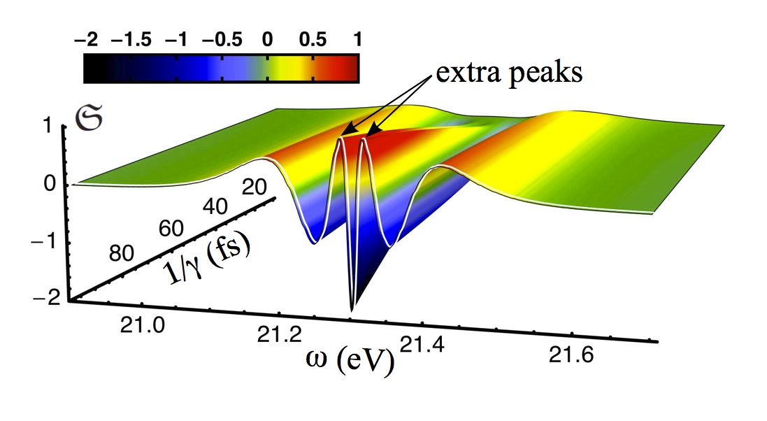
Noteworthy, the full Fourier transform of the dipole in Eq. (27) yields spectra that resemble very closely those in Figs. 3 and 4. In Fig. 5 we display the density plot of $-\omega{\rm Im}[\tilde{d}_{p}(\omega)]\propto\mathfrak{S}(\omega)$ for $\omega_{0}=21.3$ eV, $E_{0}d_{0}=0.5$ eV, $\gamma_{P}=0.41$ eV (corresponding to a duration $\Delta_{P}\sim 10$ fs) and for $\gamma=0.21$ eV (left panel, compare with Fig. 3) and $\gamma=1.37$ eV (right panel, compare with Fig. 4). Equation (27) does therefore provide a convenient analytic parametrization of experimental TPA spectra. For longer pumps Eq. (27) predicts the formation of a subsplitting structure as well. In Fig. 6 we show the TPA spectrum as a function of the dipole life-time $1/\gamma$ at delay $\tau=0$ for $\omega_{0}=21.3$ eV, $E_{0}d_{0}=0.2$ eV, $\gamma_{P}=0.125$ eV (corresponding to a duration $\Delta_{P}\sim 33$ fs). In addition to the AT peaks at $\omega_{0}\pm E_{0}d_{0}$ two extra peaks emerge, in agreement with recent experiments on a thick helium gas perturbed by a NIR pump of duration 33 fs.[66] We point out that the number of extra peaks increases with increasing the AT splitting (hence with increasing the intensity of the NIR pulse), a prediction which could be easily checked experimentally.

In this Section we extend the NEGF+GKBA formalism to deal with ionization processes induced by the pump. For this purpose it is convenient to work with the HF orbitals. Let $\rho^{\rm eq}$ be the equilibrium density matrix and

the equilibrium HF Hamiltonian in the original basis. The HF orbitals $\psi_{\mu}({\mathbf{r}})=\sum_{i}a_{i}^{\mu}\varphi_{i}({\mathbf{r}})$ diagonalize both $h^{\rm eq}_{{\rm HF}}$ and $\rho^{\rm eq}$, and are orthonormal. To distinguish the HF basis from the original basis we use greek letters to label the former. We have

and $\rho^{\rm eq}_{\mu\nu}=\delta_{\mu\nu}n_{\mu}$ where $n_{\mu}=1$ if $\epsilon_{\mu}<\epsilon_{\rm F}<0$ and $n_{\mu}=0$ otherwise, $\epsilon_{\rm F}$ being the Fermi energy.

In finite systems like atoms and molecules the HF orbitals with $\epsilon_{\mu}>0$ are states in the continuum. These are the states that get occupied by the photoelectron in a ionization process. We assume that the Coulomb interaction between photoelectrons and bound electrons is negligible and set to zero the two-electron integrals $v_{\mu\nu\alpha\beta}$ with at least one of the four indices in the continuum (this amounts to neglect Auger transitions). Then the self-energy has nonvanishing matrix elements only between bound states. In Appendix A we prove that the equation of motion for the density matrix with both indices in the bound sector reads

In Eq. (34) every matrix has indices running over the bound states. The integral $I_{\rm ion}$ accounts for the pump-induced ionization (since ${\rm Tr}[I_{\rm ion}+{\rm H.c.}]\neq 0$ the number of bound electrons is not conserved) and it is calculated like in Eq. (23) except that the correlation self-energy is replaced by the ionization self-energy $\Sigma_{\rm ion}$. The latter has a vanishing lesser part and a greater part given by (see Appendix A)

References

- [1] F. Krausz and M. Ivanov, Rev. Mod. Phys. 81, 163 (2009).
- [2] R. Berera, R. van Grondelleand, and J. T. M. Kennis, Photosynth. Res. 101, 105 (2009).
- [3] G. Sansone, T. Pfeifer, K. Simeonidis, and A. I. Kuleff, Chem. Phys. Chem. 13, 661 (2012).
- [4] L. Gallmann, J. Herrmann, R. Locher, M. Sabbar, A. Ludwig, M. Lucchini, and U. Keller, Mol. Phys. 111, 2243 (2013).
- [5] A. I. Kuleff and L. S. Cederbaum, J. Phys. B: At. Mol. Opt. Phys. 47, 124002 (2014).
- [6] M. B. Gaarde, C. Buth, J. L. Tate, and K. J. Schafer, Phys. Rev. A 83, 013419 (2011).
- [7] S. Pabst, L. Greenman, P. J. Ho, D. A. Mazziotti, and R. Santra, Phys. Rev. Lett. 106, 053003 (2011).
- [8] W. Chu and C. D. Lin, Phys. Rev. A 85, 013409 (2012).
- [9] M. Tarana and C. H. Greene, Phys. Rev. A 85, 013411 (2012).
- [10] S. Pabst, A. Sytcheva, A. Moulet, A. Wirth, E. Goulielmakis, and R. Santra, Phys. Rev. A 86, 063411 (2012).
- [11] A. N. Pfeiffer, M. J. Bell, A. R. Beck, H. Mashiko, D. M. Neumark, and S. R. Leone, Phys. Rev. A 88, 051402 (2013).
- [12] N. Rohringer and R. Santra, Phys. Rev. A 79, 053402 (2009).
- [13] R. Santra, V. S. Yakovlev, T. Pfeifer, and Z. Loh, Phys. Rev. A 83, 033405 (2011).
- [14] J. C. Baggesen, E. Lindroth, and L. B. Madsen, Phys. Rev. A 85, 013415 (2012).
- [15] E. Perfetto and G. Stefanucci, Phys. Rev. A 91, 033416 (2015).
- [16] U. De Giovannini, G. Brunetto, A. Castro, J. Walkenhorst, and A. Rubio, Chem. Phys. Chem 14, 1363 (2013).
- [17] C. Neidel, J. Klei, C.-H. Yang, A. Rouzée, M. J. J. Vrakking, K. Klünder, M. Miranda, C. L. Arnold, T. Fordell, A. L’Huillier, et al., Phys. Rev. Lett. 111, 033001 (2013).
- [18] S. M. Falke, C. A. Rozzi, D. Brida, M. Maiuri, M. Amato, E. Sommer, A. D. Sio, A. Rubio, G. Cerullo, E. Molinari, et al., Science 344, 1001 (2014).
- [19] C. A. Rozzi, S. M. Falke, N. Spallanzani, A. Rubio, E. Molinari, D. Brida, M. Maiuri, G. Cerullo, H. Schramm, J. Christoffers, et al., Nature Comm. 4, 1602 (2013).
- [20] N. T. Maitra, F. Zhang, R. J. Cave, and K. Burke, J. Chem. Phys. 120, 5932 (2004).
- [21] S. Kümmel and L. Kronik, Rev. Mod. Phys. 80, 3 (2008).
- [22] O. Gritsenko and E. J. Baerends, J. Chem. Phys. 121, 655 (2004).
- [23] N. T. Maitra, J. Chem. Phys. 122, 234104 (2005).
- [24] N. T. Maitra and D. G. Tempel, J. Chem. Phys. 125, 184111 (2006).
- [25] J. B. Neaton, M. S. Hybertsen, and S. G. Louie, Phys. Rev. Lett. 97, 216405 (2006).
- [26] A. M. Souza, I. Rungger, C. D. Pemmaraju, U. Schwingenschloegl, and S. Sanvito, Phys. Rev. B 88, 165112 (2013).
- [27] G. Stefanucci and S. Kurth, Phys. Rev. Lett. 107, 216401 (2011).
- [28] S. Kurth and G. Stefanucci, Phys. Rev. Lett. 111, 030601 (2013).
- [29] L. P. Kadanoff and G. Baym, Quantum Statistical Mechanics (W. A. Benjamin, Inc. New York, 1962).
- [30] H. Haug and A.-P. Jauho, Quantum Kinetics in Transport and Optics of Semiconductors (Springer, Berlin, 2007).
- [31] G. Stefanucci and R. van Leeuwen, Nonequilibrium Many-Body Theory of Quantum Systems: A Modern Introduction (Cambridge University Press, Cambridge, 2013).
- [32] K. Balzer, and M. Bonitz, Nonequilibrium Green’s Functions approach to Inhomogeneous Systems, Lect. Notes Phys. 867 (2013).
- [33] E. Perfetto, D. Sangalli, A. Marini, and G. Stefanucci, arXiv:1507.01786 (2015).
- [34] E. Goulielmakis, Z. Loh, A. Wirth, R. Santra, N. Rohringer, V. S. Yakovlev, S. Zherebtsov, T. Pfeifer, A. M. Azzeer, M. F. Kling, et al., Nature 466, 739 (2010).
- [35] P. Lipavský, V. pika, and B. Velický, Phys. Rev. B 34, 6933 (1986).
- [36] M. Bonitz, D. Kremp, D. C. Scott, R. Binder, W. D. Kraeft, and H. S. Köhler, J. Phys.: Condens. Matter 8, 6057 (1996).
- [37] N. H. Kwong, M. Bonitz, R. Binder, , and H. S. Köhler, Phys. Status Solidi B 206, 197 (1998).
- [38] H. Haug, Phys. Status Solidi B 173, 139 (1992).
- [39] R. Binder, H. S. Köhler, M. Bonitz, and N. Kwong, Phys. Rev. B 55, 5110 (1997).
- [40] M. Bonitz, D. Semkat, and H. Haug, Eur. Phys. J. B 9, 209 (1999).
- [41] P. Gartner, L. Bányai, and H. Haug, Phys. Rev. B 60, 14234 (1999).
- [42] Q. T. Vu and H. Haug, Phys. Rev. B 62, 7179 (2000).
- [43] A. Marini, J. Phys: Conf. Proc. 427, 012003 (2013).
- [44] D. Sangalli and A. Marini, arXiv:1409.1706 (2015).
- [45] K. Balzer, S. Hermanns, and M. Bonitz, J. Phys.: Conf. Ser. 427, 012006 (2013).
- [46] M. Bonitz, K. Balzer, and S. Hermanns, Contrib. Plasma Phys. 53, 778 (2013).
- [47] S. Hermanns, N. Schlünzen, and M. Bonitz, Phys. Rev. B 90, 125111 (2014).
- [48] S. Latini, , E. Perfetto, A.-M. Uimonen, R. van Leeuwen, and G. Stefanucci, Phys. Rev. B 89, 075306 (2014).
- [49] N. E. Dahlen and R. van Leeuwen, Phys. Rev. Lett. 98, 153004 (2007).
- [50] P. Myöhänen, A. Stan, G. Stefanucci, and R. van Leeuwen, EPL 84, 67001 (2008).
- [51] P. Myöhänen, A. Stan, G. Stefanucci, and R. van Leeuwen, Phys. Rev. B 80, 115107 (2009).
- [52] K. Balzer, M. Bonitz, R. van Leeuwen, A. Stan, and N. E. Dahlen, Phys. Rev. B 79, 245306 (2009).
- [53] M. P. von Friesen, C. Verdozzi, and C.-O. Almbladh, Phys. Rev. Lett. 103, 176404 (2009).
- [54] K. Balzer, S. Bauch, , and M. Bonitz, Phys. Rev. A 81, 022510 (2010a).
- [55] K. Balzer, S. Bauch, , and M. Bonitz, Phys. Rev. A 82, 033427 (2010b).
- [56] N. Schlünzen, S. Hermanns, M. Bonitz, C. Verdozzi, cond-mat/arXiv:1508.02947.
- [57] Y. Bar Lev and D. R. Reichman, cond-mat/arXiv:1508.05391.
- [58] P. Ranitovic, X. M. Tong, C. W. Hogle, X. Zhou, Y. Liu, N. Toshima, M. M. Murnane, and H. C. Kapteyn, Phys. Rev. Lett. 106, 193008 (2011).
- [59] A. N. Pfeiffer and S. R. Leone, Phys. Rev. A 85, 053422 (2012).
- [60] S. Chen, M. J. Bell, A. R. Beck, H. Mashiko, M. Wu, A. N. Pfeiffer, M. B. Gaarde, D. M. Neumark, S. R. Leone, and K. J. Schafer, Phys. Rev. A 86, 063408 (2012).
- [61] S. Chen, M. Wu, M. B. Gaarde, and K. J. Schafer, Phys. Rev. A 87, 033408 (2013).
- [62] M. Wu, S. Chen, M. B. Gaarde, and K. J. Schafer, Phys. Rev. A 88, 043416 (2013).
- [63] M. Chini, X. Wang, Y. Cheng, and Z. Chang, J. Phys. B: At. Mol. Opt. Phys. 47, 124009 (2014).
- [64] J. Fernández Rico, I. Ema, R. López, G. Ramírez and K. Ishida, in Recent Advances in Computational Chemistry: Molecular Integrals over Slater Orbitals, eds. T. Ozdogan and M. B. Ruiz (Transworld Research Network, 2008), pp. 145.
- [65] J. F. Rico, R. Lopez, G. Ramirez, and I. Ema, J. Comput. Chem. 25, 1987 (2004).
- [66] C.-T. Liao, A. Sandhu, S. Camp, K. J. Schafer, and M. B. Gaarde, Phys. Rev. Lett. 114, 143002 (2015).
- [67] C. F. Bunge, J. A. Barrientos, and A. V. Bunge, Atomic Data and Nuclear Data Tables 53, 113 (1993).
- [68] Similarly to He case the absolute position of the peaks is shifted with respect to experiment.
- [69] N. Säkkinen, M. Manninen, and R. van Leeuwen, New J. Phys. 14, 013032 (2012).