Generating Partially Synthetic Geocoded Public Use Data with Decreased Disclosure Risk Using Differential Smoothing
Harrison Quick1∗, Scott H. Holan2, Christopher K. Wikle2
1 Division of Heart Disease and Stroke Prevention, Centers for Disease Control and Prevention, Atlanta, GA 30329
2 Department of Statistics, University of Missouri, Columbia, Missouri.
∗ email: HQuick@cdc.gov
Summary. When collecting geocoded confidential data with the intent to disseminate, agencies often resort to altering the geographies prior to making data publicly available due to data privacy obligations. An alternative to releasing aggregated and/or perturbed data is to release multiply-imputed synthetic data, where sensitive values are replaced with draws from statistical models designed to capture important distributional features in the collected data. One issue that has received relatively little attention, however, is how to handle spatially outlying observations in the collected data, as common spatial models often have a tendency to overfit these observations. The goal of this work is to bring this issue to the forefront and propose a solution, which we refer to as “differential smoothing.” After implementing our method on simulated data, highlighting the effectiveness of our approach under various scenarios, we illustrate the framework using data consisting of sale prices of homes in San Francisco.
Key words: Bayesian methods; Data privacy; Multiple imputation; Spatial modeling; Synthetic data.
1 Introduction
When collecting confidential data with the intent to disseminate, there is often both an ethical as well as legal obligation for agencies to protect the privacy of data subjects’ identities and sensitive attributes. This charge can be particularly challenging for agencies who seek to include fine levels of geography (e.g., latitude/longitude) in the public use files they provide. While data users can benefit greatly from this detailed spatial information, this can also enable ill-intentioned users to identify individuals in the dataset. This disclosure risk can be especially high in regions where individuals with sensitive attributes may be more unique.
As a result, agencies often resort to altering (or worse, suppressing) the geographies and/or sensitive attributes before making data publicly available. A common technique is to aggregate data from the individual level to areal units (e.g., Census tracts or counties). Not only can this destroy the ability to estimate the spatial structure at finer geographies than the aggregate level, but it may also lead researchers to make ecological fallacies (Freedman,, 2004; Lawson et al.,, 2012; Bradley et al.,, 2015). Agencies may also randomly move each record’s observed location to another location, e.g., within some radius of the true location. In addition to having a negative impact on the spatial structure in the released data (Armstrong et al.,, 1999; VanWey et al.,, 2005, e.g.,), the effect of this perturbation may be overlooked by researchers, potentially resulting in false conclusions.
An alternative to releasing aggregated and/or perturbed data is to release multiply-imputed synthetic data, where sensitive values are replaced with draws from statistical models designed to capture important distributional features in the collected data. In some cases, agencies may generate fully synthetic data (Rubin,, 1993; Reiter,, 2002; Reiter,, 2005; Raghunathan et al.,, 2003; Quick et al.,, 2014), in which the released datasets are comprised entirely of simulated records. We, however, take a partially synthetic approach in which only a collection of values/variables are replaced with imputed values (Little,, 1993; Kennickell,, 1997; Abowd and Woodcock,, 2004; Reiter,, 2003; Reiter,, 2004; An and Little,, 2007; Toth,, 2014). Specifically, we assume the data consist of exact geographic locations and covariate information for each individual, as well as a continuously varying response which will be multiply imputed.
One issue that has yet to be adequately addressed, however, is how to handle spatially outlying observations in the collected data. For instance, suppose the agency would like to release annual income data for individuals from a number of subpopulations for a given city. Further, suppose a Census tract contains only one black female over 50 years of age. Were the agency to release aggregate data, it is likely that this Census tract’s income information would be suppressed for this particular subpopulation in order to protect this individual’s privacy. When generating (fully or partially) synthetic data, however, such steps to protect the individual’s privacy may not even be considered, much less taken. Furthermore, such a crude method is ignorant to the size of a given areal unit — e.g., the sole individual in an urban Census tract (where tracts may be more densely clustered) may in fact be at less risk of disclosure than one of a handful of individuals in a rural Census tract which stretches over an area of several miles. As this issue is better illustrated in a partially synthetic framework, we focus here on the partially synthetic (henceforth referred to as simply “synthetic”) case. That said, this issue still pertains to methods for generating fully synthetic data like Quick et al., (2014), though the impact is lessened due to the possibility of no synthetic observations near the locations of the spatial outliers.
We would be remiss not to mention the “robust kriging” literature, a concept proposed by Hawkins and Cressie, (1984). As discussed further by Nirel et al., (1998) and Mugglestone et al., (2000), the goal of robust kriging is to develop methods of obtaining parameter estimates which are robust to observations whose responses are outlying (or otherwise not in line with model assumptions). This is in contrast to our focus here, where we are concerned with observations whose locations are considered outlying and how this relates to disclosure risk.
The goal of this work is to bring this issue to the forefront and propose a solution. We begin in Section 2 by illustrating, in detail, the potential risks and how existing approaches fail to address the root of the problem. In Section 3, we extend existing methods for generating synthetic data to further reduce disclosure risk for spatially outlying observations using a concept we refer to as differential smoothing. We implement these methods on simulated data in Section 4, highlighting the effectiveness of our approach under various scenarios. We then apply the methodology to data consisting of sale prices of homes in San Francisco in Section 5. While privacy is not necessarily an issue for these data, they serve as a reasonable surrogate for household-level data, where disclosure risks would be of chief concern. Finally, in Section 6, we provide concluding remarks and some ideas for future research.
2 Potential Disclosure Risks in Synthetic Data
Before discussing the potential risks when generating synthetic data, we must first select a method for modeling the true data. For the sake of illustration, we shall assume that the data consists of continuous responses (e.g., annual income) from a single population. While datasets generally consist of data collected from multiple populations (e.g., race, socioeconomic status, etc.), we will restrict our attention to the univariate case; the topic of joint modeling is discussed further in Section 6.
Let and be the location and response variable for the -th individual, for . For a continuously varying and vector of model parameters, , we may choose a model of the form
| (1) |
where is a vector of spatially varying covariates with a corresponding vector of regression coefficients, , and is a random effect that induces correlation between the responses. To account for spatial correlation in the responses, a highly flexible option is to assume is a mean-zero Gaussian process, , where . For a collection of spatial locations, , we define and assume , where the -th element of is . For the sake of brevity, we suppress the conditioning and simply write and . We define to be the -dimensional vector with components for . While there are numerous choices for , we will illustrate our approach using an exponential covariance structure where . Here, represents the variance of the spatial process and denotes the spatial range, yielding as the parameters to be estimated. When is large, inverting can be computationally burdensome, and a low-rank approximation such as the modified predictive process (Banerjee et al.,, 2010) may be required. While the approach we describe in Section 3 can be implemented using a low-rank approximation, for the sake of illustration, we will assume is of a manageable size. This will allow us to focus on the properties of our approach rather than details of the low-rank approximation.
To illustrate the potential disclosure risk in synthetic data, we generate observations from (1) where , , , and locations on the unit square; the individuals are shown in Figure 1(a), overlaid on the true response surface. This choice for corresponds to for , and the values for and were chosen such that the ratio of to was large—the impact of this ratio can be seen in Section 3.2. The observation at location in Figure 1(a) is further than 0.26 units away from the remaining 499 observations, and is henceforth referred to as the “spatial outlier.” Without loss of generality, we assume this is the -th observation in the dataset. Later in Section 3.2, we will identify spatial outliers using a more relaxed definition.

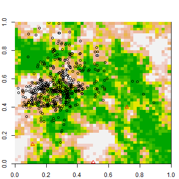
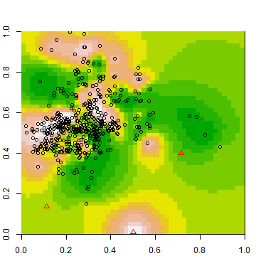
To model these data, we may use an intercept-only model, assume an exponential covariance structure for the spatial random effects, and take a Bayesian approach, completing the model specification by defining vague priors for the model parameters. After fitting the Bayesian hierarchical model and obtaining posterior distributions for the parameters, we achieve the estimated response surface shown in Figure 1(b). Of particular importance here is the presence of a ring encircling the spatial outlier, around which the predicted values appear to gradually decrease from the estimate of outside the ring to , which may be considered too close to the true value of 7.08.
Given our existing spatial locations, we can generate partially synthetic datasets by sampling synthetic responses, denoted , from the posterior predictive distribution
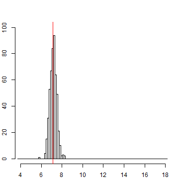
using the methods described in Quick et al., (2014) for marked point processes, where , , , and denote the -th approximately independent samples from the respective posterior distributions for , and . Figure 1(c) displays a histogram of the 500 synthetic responses for the spatial outlier. Alarmingly, this empirical distribution is almost perfectly centered around the true value for , denoted by the red line.
In essence, fitting a spatial model for data with spatial outliers may lead to overfitting in the vicinity of the outliers. Furthermore, non-model-based methods for smoothing may also yield potentially unsatisfactory results. For instance, Zhou et al., (2010) show that replacing with — where is some spatially-associated weight function with — can produce synthetic data with decreased risk. Unfortunately, if is a spatial outlier, this can still result in when for for a distance-based choice of . While this could be avoided by imposing a “disclosure constraint,” this may be detrimental to the remaining observations. Needless to say, this is a problem that is easy to overlook yet difficult to fully address.
3 Differential Smoothing Framework
3.1 Background for Bayesian spatial models
Using the model in (1), we can write and where , , , and is a diagonal matrix with elements . We can then show that the full conditional distribution for is
| (2) |
To fit this model under a Bayesian framework, we must specify prior distributions for our remaining model parameters: , , , and .
Again, we suppose that the -th observation is a spatial outlier—and thus is determined to have a high disclosure risk—while the remaining observations are clustered together and treated as having no disclosure risk. In order to account for this in the model, we define “risk weights” which will be used to differentially smooth the predicted surfaces. We then define the diagonal matrix as having elements where denotes a “global risk” parameter, and define . Now, if we want to partition the observations based on risk, we would have
| (3) |
where and denote the matrices constructed by removing the last row and column of and , respectively.
3.2 Defining the and
Rather than define on a continuum, a simple option is to let if the -th observation is deemed a spatial outlier and otherwise. For instance, we may consider the -th observation as an outlier if the distance to the nearest neighbor, for some . To define , we may choose a specification based on an inversion of the correlation structure used, such as — which ensures that for non-outliers. While there is no theoretical basis for this choice, we have found that it offers a compromise between the utility and the disclosure risk of the synthetic data we generate. Updating (3) with this restriction yields
| (4) |
We discuss the topic of continuous-valued later in Section 6.
Choosing a value for can be less clear, so first we need to investigate how different values for affect the model. To better elucidate this, suppose is sufficiently far away from the other points such that for ; i.e.,
Plugging this into the full conditional distribution for (which takes the form of (2) with replaced by ) yields
Note that this implies that the conditional expected value of is a weighted average of and the prior mean of 0; i.e.,
| (5) |
where denotes the degree of spatial smoothing. Note that setting yields , which results in the standard unrestricted model. When choosing a non-zero, finite value for , one option may be to force to take some value in to achieve a desired level of differential smoothing. For instance, if , this corresponds to , provided . To achieve a “fully smoothed” process for our outlying observations, however, we let , which corresponds to . Furthermore, note that this restriction forces ; i.e., if we let , this implies (note that does not imply ).
3.3 Implementation
To implement our differential smoothing approach, we first fit the unrestricted model:
| (6) |
with for all (or ) and using vague prior specifications for , , , and , where denotes the conditional distribution of given . We could then specify and to remain functions of our model parameters (i.e., and ), changing the degree of smoothing adaptively. As we will discuss in Section 6, however, this may have consequences regarding parameter estimation (e.g., the loss of conjugacy for ), and thus we do not pursue this here. Instead, we specify the using the distance to the nearest neighbor (as a function of the posterior median of from our unrestricted model) and implement a fully smoothed restriction by setting . We then fit the restricted hierarchical model
| (7) |
using these values of and . To facilitate faster convergence, we can use samples from the unrestricted model as initial values for the restricted model, and we recommend fixing so as not to affect which observations are to be deemed “spatial outliers”.
Using the samples drawn from the posterior distribution based from the restricted model, we then generate synthetic data from . Here again, note that if we use the fully smoothed approach where , the are simply draws from the conditional prior distribution, .
4 Simulated Example
Before delving into an assessment of the proposed method, we will first describe the motivation for the simulated example used both here and in Section 2. The response is intended to correspond to an individual’s log-transformed income, centered around an annual income of roughly $50,000 with a small proportion of the sample having incomes higher than $1,000,000 and some individuals having incomes below the poverty line. The observations are sampled such that the majority of the data come from a high density region of the spatial domain, while a few of the individuals reside in less densely populated regions (with respect to the subpopulation being sampled). As is common with real data, the simulated data contain pockets of both high and low income individuals (in practice, agencies tend to release top-coded income data (Crimi and Eddy,, 2014, e.g., see), another data-privacy method which can result in bias). To achieve this in these data, we generated from the model where , with and , and
| (8) |
As displayed in Figure 1(a), we observe a spatially outlying individual at in a relatively low income bracket who we have identified as being at-risk for disclosure. Using the methods described in Section 3, we will demonstrate our differential smoothing approach for protecting this and other individuals. We will also compare these results to those from an analysis where the spatial outlier was removed from the data prior to model fitting.
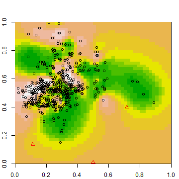
After fitting the unrestricted hierarchical model in (6), we consider the restricted model of Section 3, where we let be a 0/1 indicator function for the absence of neighbors within units, resulting in 2 additional at-risk individuals (denoted using red triangles in Figure 2). We then let , forcing for the at-risk observations, while leaving the non-at-risk observations relatively unaffected. Refitting the model under this specification, we obtain the estimated response surface in Figure 2(b). Comparing this figure to the unrestricted surface in Figure 2(a), a number of features are noticeable. First, as shown in Table 1, the estimate of has decreased from to , largely due to the negative pull of the outlying observation at , resulting in lower predictions for the unobserved regions on the right side of the spatial domain. Secondly, the ring of low predicted values around the spatial outlier has vanished, resulting in a surface that is essentially naive to the existence of this individual. Additionally, note that the estimate of in our restricted model is similar to that from the analysis of the suppressed dataset, while the estimates of and differ substantially. This is because we cannot learn about in either model, leaving and to do more work in the restricted model.

| Model | |||
|---|---|---|---|
| Full Unrestricted | 11.35 (11.13, 11.71) | 3.83 (3.22, 4.59) | 0.06 (0.05, 0.08) |
| Restricted | 10.31 (10.20, 10.77) | 3.77 (3.07, 4.53) | 0.12 (0.10, 0.15) |
| Suppressed | 11.71 (11.49, 12.07) | 3.81 (3.19, 4.58) | 0.06 (0.05, 0.08) |
We now turn our attention to the synthetic data generated from these models. Figure 3 displays the distributions of the synthetic responses for the spatial outlier. In each panel, the true value for this individual is denoted by the red vertical line, while the histogram for the restricted model also contains a green line denoting the mean of the unrestricted synthetic responses (for comparison purposes) and a blue line denoting the mean for the set of restricted responses. Here, we see the impact of the smoothing techniques in the restricted model, as now the synthetic responses are centered around the estimate for from Table 1 instead of the true value of . Recalling that these responses are modeled after log-transformed annual incomes, we can assess the disclosure risk for this individual by computing the proportion of synthetic incomes within a certain of the truth (Quick et al.,, 2014, see, e.g.,). For instance, 100% of the synthetic incomes from the unrestricted model are within $10,000 of the true value, compared to only 30% for our restricted model. Similarly, the proportion of synthetic incomes within 10% of their true values for our three at-risk individuals has been reduced by at least 73% and by an average of 20% for the non-at-risk individuals. To assess the utility of the synthetic data from our models, we fit
for and used the combination rules in Reiter, (2003) to obtain point and interval estimates for our regression parameters from each model. Table 2 displays these results for our unrestricted and restricted models, as well as those corresponding to the analysis of the suppressed data. In general, our regression parameters, , are relatively unaffected, though this is not surprising given the small number of at-risk observations.


| Parameter | Full Unrestricted | Restricted | Suppressed Unrestricted |
|---|---|---|---|
| (Intercept) | 10.58 (10.31, 10.85) | 10.57 (10.3, 10.84) | 10.54 (10.27, 10.80) |
| ( slope) | -0.16 (-0.33, 0.02) | -0.16 (-0.34, 0.02) | -0.14 (-0.32, 0.04) |
| ( slope) | 0.37 (0.20, 0.55) | 0.40 (0.22, 0.57) | 0.42 (0.24, 0.60) |
| 7.18 (6.57, 7.80) | 10.33 (6.21, 13.91) | 11.86 (8.26, 15.63) |
5 Real Data Example
Having illustrated the potential risks of the common, unrestricted model and demonstrating the effectiveness of our differential smoothing approach, we now look to apply our methodology to a dataset of home sale prices in San Francisco for the period from Feb. 2008 to July 2009. These data were collected and described by Adler, (2010) and consist of the sale price, the square footage, the number of bedrooms, and the spatial location (latitude and longitude) for each home. For the purposes of this paper, we will restrict our attention to the 214 homes with one bedroom. While these data themselves are not considered “at-risk” for disclosure (e.g., home listings are publicly available), the number of bedrooms and the home value may reasonably be considered as surrogates for sensitive household information such as the size of a household and the total household income, respectively. Thus, we believe the dependencies underlying these data are representative of those underlying data for which disclosure risk would be of concern.
Following the process used in Section 4, we first model the log-transformed sale prices using the unrestricted hierarchical model in (6) using the square footage as a covariate, yielding the prediction surface for in Figure 4(a). Here again, we see “rings” in the prediction surface surrounding a number of potential spatial outliers (denoted by red triangles). Based on the results presented in Section 2, one can intuit that synthetic responses generated from this prediction surface for these outliers may be unacceptably close to their true values, thus motivating the use of differential smoothing. Fortunately, the ratio of () to () is not as dramatic as in our simulated example, so the synthetic responses for the outlying observations are slightly shifted away from toward , as shown in Figure 5(a) for the observation at .


We then proceed to fit the restricted model. Based on the distances to their nearest neighbors, we identify seven homes as spatial outliers. Using this approach, we obtain the predicted surface for in Figure 4(b) and the synthetic data in Figure 5(b). As in the simulated example, this approach yields synthetic responses centered around the estimated value of in the restricted model. To quantify this in terms of the risk of disclosure, the percentage of synthetic responses for the observation at which are within 10% of the true value has been reduced by 93% — dropping from 46.2% of our synthetic responses in the unrestricted model to just 3% in our restricted model. Overall, this risk was reduced 50% for at-risk individuals and 11% for non-at-risk individuals.


Now, in order for our restricted model to be a valuable tool, it is important to demonstrate that it can provide synthetic data which yield statistical inference similar to that from the real data. To evaluate the utility of our synthetic data, we fit
for for each set of synthetic responses and again used the combination rules in Reiter, (2003) to obtain point and interval estimates for our regression parameters. Here, our results are even more impressive than in Table 2, as our restricted synthetic data produce estimates 13.233 (13.197, 13.269) and 0.269 (0.233, 0.306) — estimates which are each within 0.002 of those from the real data. To put these results in context, consider that the estimate for obtained from synthetic data generated from a model using a suppressed dataset is 0.279 (0.244, 0.314).
6 Discussion
In this paper, we have shed light on a unique issue regarding disclosure risk encountered when generating spatially-referenced synthetic microdata from a population with spatially outlying observations. After first illustrating an example of when this risk can arise in Section 2, we proposed a framework which could be used to alleviate the risk of disclosure by restricting the hierarchical model using differential smoothing. We then demonstrated its use on simulated data and applied it to a dataset of home sale prices in San Francisco.
Along with producing data which limit the risk of disclosure, producing data with high utility is of the utmost importance. While the synthetic data that we have generated in Sections 4 and 5 have been able to provide inference which was on par with those from the real data, this is a much more nuanced problem in practice. For instance, suppose our data consist of the gross annual household incomes for households in a particular region (and for the sake of illustration, suppose these data are not top-coded). If many of our spatial outliers also happen to be high earners (say, household incomes greater than $250,000 per year), our synthetic data will likely underestimate the number of high earners in the population. Fortunately, such issues can be addressed by constructing our hierarchical models based on important questions of inferential interest. If we desire synthetic data which preserve the number of households in certain income brackets, we can specify conditional models such as
| (9) |
where is an indicator function ensuring that belongs to a particular group, denoted . That is, we could model each household’s income using a truncated normal distribution, generating synthetic households that belong to the correct income brackets and preserving the proportions observed in the real population. While such a model would reduce data privacy — i.e., we must be willing to disclose a household’s true income bracket — data stewards know this risk beforehand and can take appropriate measures.
While our work here was focused on scenarios with a single population and Gaussian outcomes, the framework we have presented can easily be extended to a multivariate framework and/or for use in generalized linear mixed models. For instance, the value of a residence in San Francisco is likely a function of the location (), number of bedrooms (), the square footage (), and the age of the property (in years; ). To model the age of the property using differential smoothing, we could let
| (10) |
where is an intercept term and is a differentially smoothed spatial process. Then, to model the property’s value, we could let
| (11) |
where and is a differentially smoothed multivariate spatial process. In this model, predictions for an outlying observation at location with bedrooms would be based on its group-specific regression model, as well as a function of the observations near with a different number of bedrooms. For instance, in a region comprised primarily of small condominiums, the spatial surfaces for studio (no bedroom) and one-bedroom units could help inform the surface for rarer two-bedroom units.
We conclude by acknowledging that this work is just a first step toward achieving reduced disclosure risk. One drawback of the restricted model used here is that it treats the idea of being a spatial outlier as a binary decision. In our future work, we aim to devise an approach which defines continuously over the range . One option would be to define
and as explicit functions of the parameters , , and , and account for these definitions in our MCMC sampler. While this is conceptually straightforward, it is unclear how such a framework would affect the convergence of our model parameters, much less whether these particular definitions are optimal.
Acknowledgements
This research was partially supported by the U.S. National Science Foundation (NSF) and the U.S. Census Bureau under NSF grant SES-1132031, funded through the NSF-Census Research Network (NCRN) program.
References
- Abowd and Woodcock, (2004) Abowd, J. M. and Woodcock, S. D. (2004). “Multiply-imputing confidential characteristics and file links in longitudinal linked data.” In Privacy in Statistical Databases, eds. J. Domingo-Ferrer and V. Torra, 290–297. New York: Springer-Verlag.
- Adler, (2010) Adler, J. (2010). R in a Nutshell. O’Reilly Media.
- An and Little, (2007) An, D. and Little, R. (2007). “Multiple imputation: an alternative to top coding for statistical disclosure control.” Journal of the Royal Statistical Society, Series A, 170, 923–940.
- Armstrong et al., (1999) Armstrong, M. P., Rushton, G., and Zimmerman, D. L. (1999). “Geographically masking health data to preserve confidentiality.” Statistics in Medicine, 18, 495–525.
- Banerjee et al., (2010) Banerjee, S., Finley, A. O., Waldmann, P., and Ericsson, T. (2010). “Hierarchical spatial process models for multiple traits in large genetic trials.” Journal of the American Statistical Association, 105, 506–521.
- Bradley et al., (2015) Bradley, J. R., Wikle, C. K., and Holan, S. H. (2015). “Regionalization of multiscale spatial processes using a criterion for spatial aggregation error.” ArXiv preprint, arXiv:1502.01974.
- Crimi and Eddy, (2014) Crimi, N. and Eddy, W. F. (2014). “Top-coding and public use microdata samples from the U.S. Census Bureau.” Journal of Privacy and Confidentiality, 6, 21–58.
- Freedman, (2004) Freedman, D. A. (2004). “The ecological fallacy.” In Encyclopedia of Social Science Research Methods, eds. M. Lewis-Beck, A. Bryman, and T. F. Liao, vol. 1, 293. Sage Publications.
- Hawkins and Cressie, (1984) Hawkins, D. M. and Cressie, N. (1984). “Robust kriging—A proposal.” Journal of the International Association of Mathematical Geologists, 16, 3–18.
- Kennickell, (1997) Kennickell, A. B. (1997). “Multiple imputation and disclosure protection: The case of the 1995 Survey of Consumer Finances.” In Record Linkage Techniques, 1997, eds. W. Alvey and B. Jamerson, 248–267. Washington, D.C.: National Academy Press.
- Lawson et al., (2012) Lawson, A. B., Choi, J., Cai, B., Hossain, M., Kirby, R. S., and Liu, J. (2012). “Bayesian 2-stage space-time mixture modeling with spatial misalignment of exposure in small area health data.” Journal of Agricultural, Biological, and Environmental Statistics, 17, 417–441.
- Little, (1993) Little, R. J. A. (1993). “Statistical analysis of masked data.” Journal of Official Statistics, 9, 407–426.
- Mugglestone et al., (2000) Mugglestone, M. A., Barnett, V., Nirel, R., and Murray, D. A. (2000). “Modelling and analysing outliers in spatial lattice data.” Mathematical and Computer Modelling, 32, 1–10.
- Nirel et al., (1998) Nirel, R., Mugglestone, M. A., and Barnett, V. (1998). “Outlier-robust spectral estimation for spatial lattice processes.” Communications in Statistics: Theory and Methods, 27, 3095–3111.
- Quick et al., (2014) Quick, H., Holan, S. H., Wikle, C. K., and Reiter, J. P. (2014). “Bayesian marked point process modeling for generating fully synthetic public use data with point-referenced geography.” ArXiv preprint, arXiv:1407.7795.
- Raghunathan et al., (2003) Raghunathan, T. E., Reiter, J. P., and Rubin, D. B. (2003). “Multiple imputation for statistical disclosure limitation.” Journal of Official Statistics, 19, 1–16.
- Reiter, (2002) Reiter, J. P. (2002). “Satisfying disclosure restrictions with synthetic data sets.” Journal of Official Statistics, 18, 531–544.
- Reiter, (2003) — (2003). “Inference for partially synthetic, public use microdata sets.” Survey Methodology, 29, 181–188.
- Reiter, (2004) — (2004). “Simultaneous use of multiple imputation for missing data and disclosure limitation.” Survey Methodology, 30, 235–242.
- Reiter, (2005) — (2005). “Releasing multiply-imputed, synthetic public use microdata: An illustration and empirical study.” Journal of the Royal Statistical Society, Series A, 168, 185–205.
- Rubin, (1993) Rubin, D. B. (1993). “Statistical disclosure limitation.” Journal of Official Statistics, 9, 461–468.
- Toth, (2014) Toth, D. (2014). “Data smearing: an approach to disclosure limitation for tabular data.” Journal of Official Statistics, 30, 839–857.
- VanWey et al., (2005) VanWey, L. K., Rindfuss, R. R., Guttman, M. P., Entwisle, B., and Balk, D. L. (2005). “Confidentiality and spatially explicit data: concerns and challenges.” Proceedings of the National Academy of Sciences, 102, 15337–15342.
- Zhou et al., (2010) Zhou, Y., Dominici, F., and Louis, T. A. (2010). “A smoothing approach for masking spatial data.” Annals of Applied Statistics, 4, 1451 – 1475.