Role of correlations and off-diagonal terms in binary disordered one dimensional systems

In one dimensional disordered systems particles cannot freely propagate. The particle undergoes a series of scattering processes and, as a result of the destructive interference, its density profile decays exponentially. This phenomenon is called the Anderson localization (AL) [1, 2]. AL is a single particle effect and therefore cannot be observed directly in solids (because of the strong electron-electron and electron phonon interactions).

Nevertheless, nowadays many different tight-binding models can be easily implemented and investigated with ultracold atoms in optical lattices. Ultracold atomic systems in optical lattices guarantee a high degree of controllability [3, 4, 5], allowing to change experimentally parameters of the model, such as hopping amplitudes using periodic lattice modulations [6, 7, 8], or interparticle interaction strength using the magnetic Feshbach resonance [9]. In particular, the interactions can be switched off completely, creating perfect conditions for the investigation of AL. Indeed, AL of matter waves has been already observed in the laboratory [10, 11] (as well as a similar Aubry-André localization [12, 13]).

It is very convenient to study disorder phenomena with optical lattices. In particular, the diagonal disorder in ultracold systems can be very easily implemented by manipulating on-site energies, e.g. with incommensurate lattices [13] or interactions with other (heavy) species of particles [14, 15, 16, 17, 18]. The later method allows to introduce various types of correlations in the disorder distribution, e.g. dual random dimer models (DRDM), where two heavy atom never come in pairs) or $N$-mers, where heavy particles always occupy a series of neighboring $N$ sites. $N$-mer correlations have been studied in various systems such as photons in dielectric waveguide [19, 20], acoustic waves [21] or electrons in crystalline lattice [22]. The off-diagonal disorder arises quite naturally, as the differences in the on-site energies change the tunneling amplitude values. As such, the off-diagonal disorder is correlated with the diagonal disorder and its relative amplitude is small. On the contrary, in this paper we present a theoretical scheme allowing to control the off-diagonal disorder strength in an experiment (for the DRDM case see [23]).

In Section II we describe a tight binding model with the binary disorder in both on-site energies and tunneling strengths. Also, the methods of creating such a system using ultracold atoms in optical lattices is sketched. In Section III we describe a method employing transfer matrices to find resonant energies in the systems with binary correlated disorder, and use it to calculate positions of all transparent states in the case of $N$-mers with no off-diagonal disorder. In Section IV we extend our analysis to include the diagonal - off-diagonal correlated disorder. We derive an equation for the resonant energies, discuss the asymptotic behavior and compare the results with numerical calculations of the localization length. Furthermore, in Section V we describe a dual random dimer model (being a $1$-mer model with off-diagonal correlated disorder). Again, we find [23] transparent modes, present an approximate expression for the localization length and compare the results with the numerical calculations. In the Appendix, a detailed description of the Floquet formalism used to derive effective Hamiltonian with off-diagonal disorder is presented.

Consider a non-interacting tight-binding one dimensional Hamiltonian

$\displaystyle H_{0}=\sum_{i}\left(\epsilon_{i}n_{i}-(a^{\dagger}_{i}a_{i+1}+\mathrm{h.c.})\right),$

(1)

where $a_{i}$($a^{\dagger}_{i}$) is an operator of particle annihilation (creation) at site $i$, $n_{i}=a^{\dagger}_{i}a_{i}$ a particle number operator and $\epsilon_{i}$ are on-site energies (we set $\hbar=1$ and use tunneling amplitude as an energy scale). The binary disorder occurs when $\{\epsilon_{i}\}$ are random numbers and take only two values: $\epsilon_{a}$ or $\epsilon_{b}$. Because of its simplicity, the binary disordered models serve as a playground for studying the localization and transport properties.

To create the binary disorder in an optical lattice one can use two species of atoms repulsively interacting with each other. We allow only one fraction of atoms to move freely on the lattice, while the second one is trapped in the lattice sites (we call them frozen and denote with a $f$ superscript). The dynamics of the system is described by a Hamiltonian

$$H=\sum_{i}\left(V_{0}n^{f}_{i}n_{i}-(a^{\dagger}_{i}a_{i+1}+\mathrm{h.c.})\right),$$

(2)

where we eliminated interactions between the mobile particles (experimentally, one can switch them off by the optical or microwave Feshbach resonance [9] or use spin polarized fermions). As $n^{f}$ is fixed, we can treat $V_{0}n^{f}_{i}$ as an effective on-site energy $\epsilon_{i}$. Furthermore, if the frozen particles are fermions or strongly repelling (hard-core) bosons, then their occupation per a lattice site $n^{f}_{i}$ is either zero or one and hence the on-site energies take only two values $\epsilon_{i}\in\{0,V_{0}\}$.

The strength of the interspecies interaction $V_{0}$ can be changed in an experiment by applying a proper magnetic field $B$, which is close to the value of the Feshbach resonance. In our scheme, we choose the magnetic field to be time periodic $B(t)=B(t+T)$, in such a way that the interactions are changing harmonically:

$$\epsilon_{i}\rightarrow\epsilon_{i}(t)=n^{f}_{i}(V_{0}+V_{1}\sin(\omega t)).$$

(3)

As changing the magnetic field in a vicinity of the Feshbach resonance leads to rapid changes of the interaction strength, the relative values of $V_{0}$ and $V_{1}$ can be chosen at will in a broad range of values. In this way we obtain a time-dependent Hamiltonian:

$$H(t)=\sum_{i}\left(n^{f}_{i}(V_{0}+V_{1}\sin(\omega t))n_{i}-(a^{\dagger}_{i}a_{i+1}+\mathrm{h.c.})\right).$$

(4)

If the modulation frequency $\omega$ is bigger than other energy scales in system ($\omega\gg 1$) then, by the means of the Floquet theory, one can average out fast oscillating terms and find an effective Hamiltonian governing the long term dynamics of the system (see Appendix):

$$H_{eff}=\sum_{i}\left(\epsilon_{i}n_{i}-t_{i}(a^{\dagger}_{i}a_{i+1}+\mathrm{h.c.})\right),$$

(5)

where $\epsilon_{i}=n^{f}_{i}V_{0}$ and $t_{i}=\mathcal{J}_{0}\left(\frac{V_{1}}{\omega}(n^{f}_{i+1}-n^{f}_{i})\right)$ is a renormalized hopping. For a binary case $n^{f}_{i}\in\{0,1\}$:

$$\epsilon_{i}=\left\{\begin{matrix}0,&\mbox{ if }n^{f}_{i}=0\\ V_{0},&\mbox{ if }n^{f}_{i}=1\end{matrix}\right.,\quad t_{i}=\left\{\begin{matrix}1,&\mbox{ if }n^{f}_{i}=n^{f}_{i+1}\\ t^{\prime},&\mbox{ if }n^{f}_{i}\neq n^{f}_{i+1}\end{matrix}\right.,$$

(6)

where $t^{\prime}=\mathcal{J}_{0}\left(V_{1}/\omega\right)$ varies from 1 to about -0.4 (to the minimum of the Bessel function, $\min_{x}\mathcal{J}_{0}(x)$).

Due to Anderson theory of localization in one dimensional system all states should be localized, unless disorder have some correlations. In the binary disordered systems correlations can take a form of $N$-mers where frozen particles always come in series of length $N$, or dual random dimer model (DRDM) where no two frozen particles can appear on the adjacent sites. Such correlations can be created by using several lattices with different lattice constants (as described for the case of the DRDM in [24]).

A transfer matrix method is a very effective tool for the numerical computation of the localization length [25]. The formalism can be also used to find analytically the delocalized modes that are appearing in systems with the correlated binary disorder. A transfer matrix for a system described by (5) has a form:

$$\left(\begin{array}[]{c}\psi_{i+1}\\ \psi_{i}\end{array}\right)=\left(\begin{array}[]{c c}\frac{\epsilon_{i}-E}{t_{i}}&-\frac{t_{i-1}}{t_{i}}\\ 1&0\end{array}\right)\left(\begin{array}[]{c}\psi_{i}\\ \psi_{i-1}\end{array}\right)\equiv T_{i}\left(\begin{array}[]{c}\psi_{i}\\ \psi_{i-1}\end{array}\right),$$

(7)

where $E$ is an energy of a state. Iterating the procedure:

$$\left(\begin{array}[]{c}\psi_{j+1}\\ \psi_{j}\end{array}\right)=T_{j}\cdot\ldots\cdot T_{i}\left(\begin{array}[]{c}\psi_{i}\\ \psi_{i-1}\end{array}\right)\equiv T_{i}^{j}\left(\begin{array}[]{c}\psi_{i}\\ \psi_{i-1}\end{array}\right).$$

(8)

In our analysis, we consider systems with binary disordered correlations in a form of $N$-mers where frozen particles always come in series of length $N$. All such blocks have the same internal structure - it is the distribution of them which is random. Therefore, one can study transfer matrix of single block ranging from $i+1$ to $i+N$ (i.e. $T^{i+N}_{i}=T_{i+N}\cdot\ldots\cdot T_{i+1}$) to get some insight in the transport properties of the whole system. For the case of an $N$-mer with uniform tunnelings ($t^{\prime}=1$), such a matrix can be written explicitly:

$$T^{i+N}_{i+1}\equiv T^{N}(\varepsilon)=\left(\begin{array}[]{c c}w_{N}(\varepsilon)&-w_{N-1}(\varepsilon)\\ w_{N-1}(\varepsilon)&-w_{N-2}(\varepsilon)\end{array}\right),$$

(9)

where $\varepsilon=E-V_{0}$ and $w_{n}(\varepsilon)$ is a polynomial of the $n$-th order given by a recursive formula:

$$w_{n}(\varepsilon)=-\varepsilon\,w_{n-1}(\varepsilon)-w_{n-2}(\varepsilon),$$

(10)

where $w_{-1}(\varepsilon)=0$ and $w_{-2}(\varepsilon)=-1$. Solving the equation (10) we can get an explicit expression:

$$w_{m}(\varepsilon)=\sum_{k=0}^{\lfloor m/2\rfloor}\left(\begin{matrix}m-k\\ k\end{matrix}\right)(-1)^{k+m}\,\varepsilon^{m-2k}.$$

(11)

In particular, a transfer matrix for a system without disorder (for an arbitrary number of sites) reads

$$T^{M}(E)=\left(\begin{array}[]{c c}w_{M}(E)&-w_{M-1}(E)\\ w_{M-1}(E)&-w_{M-2}(E)\end{array}\right).$$

(12)

We can compare a free transfer matrix (12) with the $N$-mer transfer matrix (9)

$\displaystyle T^{N}(E-V_{0})=T^{M}(E).$

(13)

If the condition (13) is met for some energy $E_{r}$, then we can say that for a state with such an energy the $N$-mer disordered system has the same transport properties as a free system. Hence, this state is delocalized. Such a procedure can be easily extended to any kind of correlations in a form of randomly distributed blocks with fixed internal structure, not necessarily $N$-mers.

A problem of finding transparent modes for binary disordered system with $N$-mer correlations can be fully solved by writing explicitly equations (13), using (10) and the fact that determinant of $T^{N}(\varepsilon)$ is one ($\det(T^{N}(\varepsilon))=1$). Then, it can be shown that the only nontrivial solutions (i.e. $V_{0}\neq 0$) of the equation (13) exist if

$$w_{N-1}(E-V_{0})=0,$$

(14)

therefore a problem of finding resonant energies is reduced to finding zeros of the polynomial $w_{N-1}$. It immediately follows that:

$$T^{N}(E_{r}-V_{0})=\pm\left(\begin{array}[]{cc}1&0\\ 0&1\end{array}\right),$$

(15)

which means that (13) is trivially satisfied for $M=0$. It turns our that a $N$-mer problem has $N-1$ resonant energies (this result, from a different approach, has been first presented in [26]):

$$E_{r}=V_{0}+2\cos(\frac{\pi}{N}i)\quad\mathrm{for}\;i\in\{1,\ldots,N-1\}.$$

(16)

The additional condition for the appearance of extended states is that its energy has to lie in the energy band for a system without disorder ($|E_{r}|\leq 2$).

The properties of the system change dramatically if we add the off-diagonal disorder, as in (5). The off-diagonal disorder arises naturally in the model, as the differences in the on-site energies alter the hooping terms, but usually their values are small comparing to the diagonal disorder. Nevertheless, in our approach we can independently manipulate the values of diagonal and off-diagonal disorder. For the $N$-mer, due to (6), only the edge tunneling amplitudes are changed: $t_{i}=t_{i+N}=t^{\prime}$ (we assume here that $N$-mers are separated by at least one empty site). To obtain a transfer matrix of the $N$-mer, we need to write a transfer matrix for $N+2$ sites (since the altered tunneling amplitudes $t^{\prime}$ appear in $T_{i}$, $T_{i+1}$, $T_{i+N}$ and $T_{i+N+1}$ we have to include two extra matrices):

$$\tilde{T}^{N}(\varepsilon)\equiv T_{i}^{i+N+1}=T_{i+N+1}T_{i+N}\underbrace{T_{i+N-1}\ldots T_{i+2}}_{T^{N-2}(\varepsilon)}T_{i+1}T_{i},$$

(17)

resulting in (where we denote the matrix elements with $v_{M}$, $v_{M-1}$, $v_{M-2}$ for the later convenience)

$$\tilde{T}^{N}(\varepsilon)=\left[\begin{matrix}v_{M}&-v_{M-1}\\ v_{M-1}&-v_{M-2}\end{matrix}\right],$$

(18)

where

	$\displaystyle v_{M-2}$	$\displaystyle=$	$\displaystyle\frac{1}{t^{\prime 2}}w_{N}(\varepsilon),$		(19)
	$\displaystyle v_{N-1}$	$\displaystyle=$	$\displaystyle-\frac{E}{t^{\prime 2}}w_{N}(\varepsilon)-w_{N-1}(\varepsilon),$
	$\displaystyle v_{N}$	$\displaystyle=$	$\displaystyle\frac{E^{2}}{t^{\prime 2}}w_{N}(\varepsilon)+2Ew_{N-1}(\varepsilon)+t^{\prime 2}w_{N-2}(\varepsilon).$

It is straightforward to check that a condition

$$\tilde{T}^{N}(\varepsilon)=T^{M}(E)$$

(20)

is not satisfied by energies given by (16). To fully solve the equation (20), we use the same procedure as in Section III. We assume that (19) fulfill a recursive formula:

$$v_{n}=-Ev_{n-1}-v_{n-2}.$$

(21)

It is a necessary but not sufficient condition for the resonance, as we do not know if there exist $M\in\mathbb{Z}$ such that (20) is satisfied (in other words, we do not know if initial conditions of (21) meet that of (10)).

From (21) we can get an equation for zeros of polynomial of $N$-th order in $\varepsilon$:

$$((1-t^{\prime 2})\varepsilon-t^{\prime 2}V_{0})w_{N-1}(\varepsilon)+(1-t^{\prime 4})w_{N-2}(\varepsilon)=0.$$

(22)

First, we can analyze limiting cases: for $t^{\prime}=1$ we restore the equation (14), so the approach is consistent with the one presented in Section III. In the case of $t^{\prime}\rightarrow\pm\infty$ we get $w_{N-2}(\varepsilon)=0$, so the resonances can appear for the same energies as for the $(N-1)$-mer with uniform tunnelings. The case of $t^{\prime}=0$ is trivial, as the chain is broken into pieces, and hence no transport can occur. Still, we can find that (22) comes down to $w_{N}(\varepsilon)=0$, so for $t^{\prime}\rightarrow 0$ the resonant energies approach those of the $(N+1)$-mer.

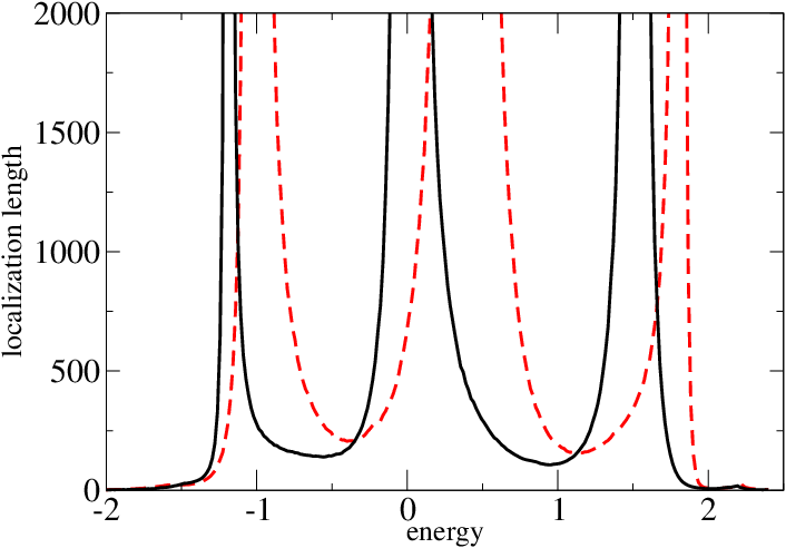
Solving (22) numerically gives always $N$ solutions, for $t^{\prime}\rightarrow 1$ one of them diverges and the rest converges to $N-1$ solutions for the $N$-mer with uniform tunnelings. If $t^{\prime}\rightarrow\infty$ two edge solutions diverge and the rest of them go asymptotically to the solutions for the $(N-1)$-mer. An example for the $4$-mer with $V_{0}=0.3$ is presented in Fig. 1.

Nevertheless, only for $t^{\prime}=1$ we can say that states with $E_{r}$ move through the system in a way as there were no disorder. For $t^{\prime}\neq 1$ situation is ambiguous, the equation (21) is satisfied, but we are unable to find $M$ for which $\tilde{T}^{N}(\varepsilon)=T^{M}(E)$. However, for $K\rightarrow\infty$, the difference asymptotically diminishes:

$$\min_{M\leq K}\|\tilde{T}^{N}(\varepsilon)-T^{M}(E)\|_{2}\xrightarrow{K\rightarrow\infty}0.$$

(23)

where $\|.\|_{2}$ is Frobenius matrix norm. Numerical results for the $4$-mer with $V_{0}=0.5$, $t^{\prime}=0.5$ (for $E_{R}=-1.1485$) are shown in Fig. 2.

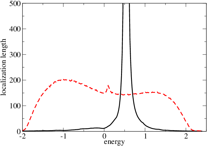
In Fig. 3 we present numerically calculated Anderson localization lengths (using the standard transfer matrix method, see e.g. [25]) for the 4-mer and the mean occupation $0.55$, the strength of disorder is set to $V_{0}=0.4$. The red dashed line corresponds to the system with uniform tunnelings $t^{\prime}=1$ while the black solid line is obtained for $t^{\prime}=0.9$. Resonances in case of $t^{\prime}=1$ are present at positions given by (16) while positions of resonances for $t^{\prime}=0.9$ agree with those obtained using (22). Values of localization length in the vicinity of $E_{r}$ for the case of $t^{\prime}=0.9$ shows that the resonance indeed exists. Localization length seems to diverge as increasing the resolution makes it bigger.

All the above analysis was valid for $N$-mers with $N\geq 2$, the case of $1$-mer is special. For the case of uniform tunnelings $t^{\prime}=1$ it does not have any delocalized modes – which is obvious as it is just the uncorrelated disorder. Even if we add an auxiliary condition that no two frozen particles can occupy adjacent sites (which is equivalent to a condition of separation of $N$-mers), situation does not change – it follows trivially from (13). However if $t^{\prime}\neq 1$, we get the so called dual random dimer model (DRDM). It has been extensively studied[27, 24, 23]. Such a model has the resonant energy

$$E_{r}=\frac{V_{0}}{1-t^{\prime 2}},$$

(24)

for which:

$$\tilde{T}^{1}(E_{r}-V_{0})=T^{3}(E_{r})$$

(25)

is satisfied. As $M$ is finite, this resonance is similar to resonances for $N$-mers with uniform tunnelings rather than for case with $t^{\prime}\neq 1$. The resonance (24) is present as long as the resonant energy lies withing the band width $|E_{r}|\leq 2$ which is equivalent to the condition: $V_{0}\leq 2\left|1-t^{\prime 2}\right|$.

The presence of the resonant mode results in the divergence of the AL length. In the limit of a small disorder (both diagonal $V_{0}\approx 0$ and off-diagonal $t^{\prime}\approx 1$) it is possible to obtain an analytical expression for the inverse localization length [23]

	$\displaystyle\lambda^{-1}$	$\displaystyle=$	$\displaystyle\frac{\rho}{(1+\rho)^{2}}\frac{(V_{0}+2(1-t^{\prime 2})\cos(k))^{2}}{8\sin^{2}(k)}$		(26)
		$\displaystyle\times$	$\displaystyle\left(1-2\frac{\rho(\rho+\cos(2k))}{1+\rho^{2}+2\rho\cos(2k)}\right),$

where we substituted $E=2\cos(k)$ for an eigenenergy $E$, and $\rho=\tilde{\rho}/(1-\tilde{\rho})$ where $\tilde{\rho}$ is the mean occupation number of frozen particles. Indeed, the expression (26) vanishes for the resonant energy $E_{r}$.

In this work we have described a method of preparing the binary disorder in optical lattices using two atomic species. In such systems, the off-diagonal disorder can be created using the fast periodic modulation of the interspecies interactions. Consequently, effective values of diagonal and off-diagonal disorder can be changed independently in a broad range. In order to observe single particle localization, we assume that either our mobile particles are spin polarized fermions or that we switch off interactions using the optical Feshbach resonance.

We made a detailed analysis of the localization properties in systems with the disorder with correlations in a form of $N$-mers, especially determining the resonant energies for which the unobstructed transport through the system occurs. For that purpose, we employed the transfer matrix formalism. In this way, we restored a known result in the case of no off-diagonal disorder [26]. Furthermore, we extended the analysis to the case with disorder in tunnelings and derived an equation for the values of the resonant energies and analyze their asymptotic values.

We showed that, except the case of $t^{\prime}=1$, initial conditions of recurrence equation (10) are met only asymptotically. It is not clear whether these states are extended, but it seems that particles with the nearly resonant energies always escape finite systems.

We acknowledge a support of the Polish National Science Centre via project DEC-2012/04/A/ST2/00088. AK acknowledges support in a form of a special scholarship of Marian Smoluchowski Scientific Consortium Matter Energy Future from KNOW funding. Support from the EU Horizon 2020-FET QUIC 641122 is also acknowledged.

References

- [1] P. Anderson, Physical Review 109, 1492 (1958).
- [2] A. Lagendijk, B. van Tiggelen, and D. Wiersma, Phys. Today 62, 24 (2009).
- [3] I. Bloch, J. Dalibard, and W. Zwerger, Rev. Mod. Phys. 80, 885 (2008).
- [4] D. Jaksch and P. Zoller, Annals of Physics 315, 52 (2005).
- [5] M. Lewenstein, A. Sanpera, and V. Ahufinger, Ultracold Atoms in Optical Lattices: Simulating Many-Body Quantum Systems (Oxford University Press, 2012).
- [6] A. Eckardt, C. Weiss, and M. Holthaus, Phys. Rev. Lett. 95, 260404 (2005).
- [7] H. Lignier, C. Sias, D. Ciampini, Y. Singh, A. Zenesini, O. Morsch, and E. Arimondo, Phys. Rev. Lett. 99, 220403 (2007).
- [8] J. Struck, C. Ölschläger, R. Le Targat, P. Soltan-Panahi, A. Eckardt, M. Lewenstein, P. Windpassinger, and K. Sengstock, Science 333, 996 (2011).
- [9] C. Chin, R. Grimm, P. Julienne, and E. Tiesinga, Rev. Mod. Phys. 82, 1225 (2010).
- [10] J. Billy, V. Josse, Z. Zuo, A. Bernard, B. Hambrecht, P. Lugan, D. Clément, L. Sanchez-Palencia, P. Bouyer, and A. Aspect, Nature 453, 891 (2008).
- [11] F. Jendrzejewski, A. Bernard, K. Mueller, C. Patrick, V. Josse, M. Piraud, L. Pezze, L. Sanchez-Palencia, A. Aspect, and P. Bouyer, Nature Phys. 8 (2012).
- [12] S. Aubry and G. André, Ann. Israel Phys. Soc. 3, 133 (1980).
- [13] G. Roati, C. D’Errico, L. Fallani, M. Fattori, C. For, M. Zaccanti, G. Modugno, M. Modugno, and M. Inguscio, Nature 453, 895 (2008).
- [14] U. Gavish and Y. Castin, Phys. Rev. Lett. 95, 020401 (2005).
- [15] P. Massignan and Y. Castin, Physical Review A 74, 013616 (2006).
- [16] S. Ospelkaus, C. Ospelkaus, O. Wille, M. Succo, P. Ernst, K. Sengstock, and K. Bongs, Phys. Rev. Lett. 96, 180403 (2006).
- [17] B. Horstmann, J. I. Cirac, and T. Roscilde, Phys. Rev. A 76, 043625 (2007).
- [18] K. V. Krutitsky, M. Thorwart, R. Egger, and R. Graham, Phys. Rev. A 77, 053609 (2008).
- [19] R. W. Peng, Y. M. Liu, X. Q. Huang, F. Qiu, M. Wang, A. Hu, S. S. Jiang, D. Feng, L. Z. Ouyang, and J. Zou, Phys. Rev. B 69, 165109 (2004).
- [20] Z. Zhao, F. Gao, R. W. Peng, L. S. Cao, D. Li, Z. Wang, X. P. Hao, M. Wang, and C. Ferrari, Physical Review B - Condensed Matter and Materials Physics 75, 1 (2007).
- [21] D. F. Barros, a. E. B. Costa, and F. a. B. F. de Moura, Journal of Physics: Condensed Matter 23, 345404 (2011).
- [22] S. N. Evangelou and E. N. Economou, Journal of Physics A: Mathematical and General 26, 2803 (1993).
- [23] A. Kosior, J. Major, M. Płodzień, and J. Zakrzewski, ArXiv e-prints (2015), eprint 1502.02453, Phys. Rev. A in press.
- [24] J.-F. Schaff, Z. Akdeniz, and P. Vignolo, Phys. Rev. A 81, 041604 (2010).
- [25] C. A. Muller and D. Delande, Chapter 9 in Les Houches 2009 - Session XCI: Ultracold Gases and Quantum Information (Oxford University Press, 2011).
- [26] F. M. Izrailev, T. Kottos, and G. P. Tsironis, Physical Review B 52, 3274 (1995).
- [27] D. H. Dunlap, H.-L. Wu, and P. W. Phillips, Phys. Rev. Lett. 65, 88 (1990).
- [28] G. Floquet, Annales de l’École Normale Supérieure 12, 47 (1883).
- [29] J. H. Shirley, Phys. Rev. 138, B979 (1965).
- [30] S. Rahav, I. Gilary, and S. Fishman, Phys. Rev. A 68, 013820 (2003).
- [31] E. Anisimovas, G. Žlabys, B. M. Anderson, G. Juzeliūnas, and A. Eckardt, Phys. Rev. B 91, 245135 (2015).
- [32] M. Bukov, L. D’Alessio, and A. Polkovnikov, Advances in Physics 64, 139 (2015).
- [33] D. Poletti and C. Kollath, Phys. Rev. A 84, 013615 (2011).
Appendix A Fast modulation of on-site energies
In this section we derive an effective Hamiltonian for a cold atom realization of binary disorder with off-diagonal terms. The scheme we present allows to manipulate experimentally relative values of diagonal and off-diagonal disorder.
In Section II we consider the on-site energy variations due to disorder caused by a frozen fraction of particles. We apply periodic modulations of the on-site energies and obtain time dependent tight-binding Hamiltonian