Forward Invariant Cuts to Simplify Proofs of Safety

A hybrid program is specified by the grammar

where $\alpha,\beta$ are hybrid programs, $\theta,\theta_{1},\dots,\theta_{n}$ are terms, and $H$ is a logical formula. Intuitively, the program $x\coloneqq\theta$ means that $x$ is assigned the value of the term $\theta$. The program $x\coloneqq*$ means that $x$ is nondeterministically assigned an arbitrary real value. The program $\{x_{1}^{\prime}=\theta_{1},\dots,x_{n}^{\prime}=\theta_{n}\&H\}$ means that the variables $x_{1},\dots,x_{n}$ evolve continuously for some duration, with derivatives $\theta_{1},\dots,\theta_{n}$, subject to the constraint that $x_{1},\dots,x_{n}$ satisfy $H$ during the entire flow. The hybrid program $?H$ behaves as a skip if the logical formula $H$ is true, and as an abort otherwise.

The nondeterministic choice $\alpha\cup\beta$ means that either $\alpha$ or $\beta$ may be executed. The sequential composition $\alpha;\beta$ means that $\alpha$ is executed, then $\beta$. The nondeterministic repetition $\alpha^{*}$ means that $\alpha$ is executed an arbitrary (possibly zero) number of times. The logic d$\mathcal{L}$ itself is a multimodal logic, in which the modalities are annotated with hybrid programs. The formulas of d$\mathcal{L}$ are described by the grammar:

where $\phi$, $\psi$ are formulas of d$\mathcal{L}$ , $\theta_{1}$, $\theta_{2}$ are terms, and $\alpha$ is a hybrid program. The box modality $[\alpha]\phi$ means that $\phi$ holds after all traces of the hybrid program $\alpha$, and $\left<\alpha\right>\phi$ means that $\phi$ holds after some execution of hybrid program $\alpha$.

In the sequel, we will abuse notation and use a formula interchangeably with the set that it represents.

Model  1 shows a hybrid program representation of the running example. Line  1 shows how the subprograms are assembled into the overall program. The system starts at a set $I$ (Line  1), and at each iteration of the loop, one of the subprograms is nondeterministically chosen for attempted execution. If the guard of the subprogram succeeds, execution proceeds. The verification task is to show that when this loop is executed any (finite) number of times, the state remains in the set $S$ (Line  1). Line  1 is the guard and differential equations of $q_{0}$. Line  1 is the transition from $q_{0}$ to $q_{1}$ and the required guard. Line  1 proceeds to specify the continuous evolution of $q_{1}$. Line  1 applies the reset of the transition into $q_{2}$, which indicates that the state resets anywhere in the circle of radius two. Line  1 checks the incoming guard to $q_{2}$ and Line  1 specifies the associated differential equations. Line  1 specifies the guard that allows transitions into the failure mode. Note that the guard does not check the current mode, since all of the modes may transition into the failure mode if the continuous states leave their prescribed bounds. Line 1 specifies that once the failure mode is entered, it is not possible to leave it, and states $x_{1},x_{2}$ maintain their previous values and do not evolve.

The safety verification problem is to decide whether the state of a system is always contained within a given safe set when starting from a designated initial set, or equivalently, whether none of the behaviors enter an unsafe set.

To formalize this problem in d$\mathcal{L}$ , suppose $\alpha$ is a hybrid program representation of the system of interest. Suppose $S$ is the safe set and $I$ is the set of initial states. Then the behaviors of $\alpha$ are contained in $S$ if the following formula is a theorem of d$\mathcal{L}$ .

The theorem prover KeYmaera can be used to attempt to prove this.

To solve this problem, one might construct a set that contains all of the system behaviors from the initial set and is contained in the safe set. We call such a set a safety certificate. A safety certificate must contain the initial state set, exclude the unsafe set, and be invariant for system behaviors. We say that a set is initialized if it includes the initial set, safe if it excludes the unsafe set, and invariant if whenever a system behavior enters it, the behavior remains in the set for all future time. Arguments with safety certificates are captured in d$\mathcal{L}$ using the invariant proof rule, where $C$ is a safety certificate:

The general task of finding a safety certificate is difficult. In this work, we propose instead a procedure that incrementally works towards a proof. Instead of a safety certificate, we use knowledge of system structure to propose sets that are invariant and safe, but not necessarily initialized, and leverage them in the proof procedure.

In our running example, modes $q_{1}$ and $q_{2}$ have stable dynamics. If a Lyapunov function can be computed for either of these modes, its sublevel sets (i.e., sets of the form $\{x~|~V(x)\leq\ell\}$, for some $\ell\geq 0$) will be invariant. The sublevel sets will be safe if they exclude the transition to the fail mode, but they will not be initialized, since they do not contain mode zero.

A cut in a logical proof allows introducing a lemma. The main contribution of this paper is a type of cut that simplifies the proof procedure by leveraging knowledge of local invariance properties.

The following theorem establishes that if it can be shown that a predicate ($C$) is locally invariant ($C\rightarrow[\alpha]C$) and safe ($C\rightarrow S$), then the remaining conditions ($\neg C$) can be separately addressed to prove safety.

For the running example, mode $q_{1}$ has a Lyapunov function of the form $V_{1}(x_{1},x_{2})$ = $\frac{1}{2}x_{1}^{2}+\frac{1}{2}(x_{2}-2)^{2}$ as described in Example 4.10 of [19] (we discuss Lyapunov functions as sources of invariants in Section 4). The sublevel set $V_{1}(x_{1},x_{2})\leq 5$ contains the reset into mode $q_{1}$. We apply the forward invariant cut rule with $C_{1}=V_{1}(x_{1},x_{2})\leq 5~\wedge~M=M_{1}$, a set that is invariant and safe, but not initialized since it does not contain the initial mode $q_{0}$ of the hybrid system. The rule application causes the proof tree to split into three branches. The first branch requires showing that whenever the system begins in $C_{1}$, it remains in $C_{1}$. The only portions of the model that may run in this case correspond to $q_{1}$ and the transition into the $\mathbf{fail}$ mode (programs $\mathtt{m}_{1}$ and $\mathtt{s}_{0,1,2\mapsto fail}$. KeYmaera can readily check that since the proposed sublevel set excludes the guard into $\mathbf{fail}$, $C_{1}$ will in fact be satisfied by the end of each system trace. The second branch of the proof tree requires showing $C\rightarrow S$, which is trivial, since $S$ is simply $M\neq M_{fail}$ and $C$ stipulates $M=M_{1}$. We now turn our attention to the third branch.

Mode $q_{2}$ has a Lyapunov function $V(x_{1},x_{2})$ = $2x_{1}^{2}+4x_{2}^{2}$, computed using standard Lyapunov techniques for linear systems. The sublevel set $V_{2}(x_{1},x_{2})\leq 16$ contains the circle of radius $2$; all incoming transitions to mode $q_{2}$ make the system state to be reset to somewhere within this circle. By applying a forward invariant cut with $C_{2}$ = $V_{2}(x_{1},x_{2})\leq 16~\wedge~M=M_{2}$, we again get three branches. As before, $C_{2}$ is invariant because the only portions of the model that may run from $C_{2}$ are the programs $\mathtt{m}_{2}$ and $\mathtt{s}_{0,1,2\mapsto fail}$. Since $V_{2}(x_{1},x_{2})\leq 16$ excludes the guard to $\mathtt{fail}$, KeYmaera can show that $C_{2}$ represents a safe set. The next branch is to prove that $C_{2}$ implies safety, which is easy because $C_{2}$ requires $M=M_{2}$, which implies $M\neq M_{fail}$.

The third branch can now be easily proved with the standard tools of KeYmaera, using the loop invariant $M=M_{0}~\wedge~x_{1}^{2}+x_{2}^{2}\leq 10$.

Lyapunov analysis provides one way to construct forward invariant sets for hybrid systems. We briefly review the basics of Lyapunov analysis to aid our presentation. Lyapunov’s direct method is a well-known method used to prove stability of dynamical systems within a region of interest. In this method, the user provides a local Lyapunov function $V:X\to\mathbb{R}$ that over the domain of interest $X$ satisfies the following properties:

1. 1.

   Positive definiteness: for all $\mathbf{x}$ in $X$,

   $$V(\mathbf{x})>0,$$

   (7)

   and $V(\mathbf{0})=0$;

2. 2.

   Derivative negative semidefiniteness: for all $\mathbf{x}$ in $X$,

   $$\dot{V}(\mathbf{x})=\frac{d}{dt}V(\mathbf{x})\leq 0,$$

   (8)

   and $\dot{V}(\mathbf{0})=0$.

Existing techniques from dynamical systems theory use sum-of-squares optimization [22] and semidefinite programming [4, 30] to identify Lyapunov functions [21] for systems described by polynomial differential equations. A Lyapunov function $V$ is analogous to a ranking function for a discrete system, and it maps each continuous state $\mathbf{x}$ to a positive real number, with the property that along any system trajectory the quantity $V(\mathbf{x})$ monotonically decreases until it reaches $0$ at the equilibrium point. It is well-known that the sublevel set of a Lyapunov function, $\mathcal{S}_{\ell}$ = $\left\{\mathbf{x}|V(\mathbf{x})\leq\ell\right\}$ is a forward invariant set, i.e., given any initial condition in $\mathcal{S}_{\ell}$, all future states remain in $\mathcal{S}_{\ell}$. Thus, any sublevel set of a Lyapunov function that includes the initial set and excludes the unsafe set serves as a safety certificate [16, 26].

We now show how we can use Lyapunov-like functions to construct local certificates.

Given a local Lyapunov function $V$ valid in the domain $X$, if an $\ell$ can be selected such that (10) and (11) are satisfied, then $B(\mathbf{x})=V(\mathbf{x})-\ell$ is a barrier certificate. This follows from the definition of barrier certificates and the Lyapunov conditions (7) and (8).

Because there are no optimality guarantees from the global optimizer used to generate the candidate barrier function, the resulting candidate may not strictly satisfy the desired constraints. To check whether the candidates satisfy (10) through (12), we rely on a satisfiability modulo theories (SMT) solver that can handle nonlinear theories over the reals. We use the dReal tool, which uses interval constraint propagation (ICP) [11]. dReal supports various nonlinear elementary functions in the framework of $\delta$-complete decision procedures, and returns “unsat” or “$\delta$-sat” for a given query, where $\delta$ is a precision value specified by the user. When the answer is “unsat”, dReal produces a proof of unsatisfiability; when it returns “$\delta$-SAT”, it gives an interval of size $\delta$, which contains points that may possibly satisfy the query.

When a “$\delta$-SAT” result is returned from a query to check (10) through (12), we do the following: 1.) construct a new linear constraint based on the interval returned, 2.) add the new constraint to the existing set of linear constraints, and 3.) re-solve the LP to obtain an updated (improved) Lyapunov function candidate. If this process terminates, then the result is a barrier certificate.

Our technique attempts to use discovered barrier certificates locally, that is, for each mode we attempt to construct a certificate that proves that the system will not leave the mode. If such a local barrier certificate is found, then the forward invariant cut rule can be applied to the mode to simplify the safety proof for the system, which may be composed of several modes.

Consider an open two-mode system, where an external input can cause the system to arbitrarily switch between the system modes. This example is significant, because neither of the two modes is invariant, so the proof cannot rely on cutting out entire modes.

The continuous dynamics are defined by matrices $A_{1}$ and $A_{2}$, as given below:

Linear reset maps are applied to the state when a transition is made between Modes 1 and 2. The resets are defined by matrices $R_{12}$ and $R_{21}$:

Figure 2 shows a hybrid automaton for the system, and Model 2 defines the corresponding hybrid program. For both modes, the continuous-time dynamics given by $A_{1}$ and $A_{2}$ are stable and linear. It is well known that even for switched-mode systems with stable linear continuous dynamics, switching conditions exists that lead to instability for the switched system [5]. We wish to prove that it is not possible to switch between $A_{1}$ and $A_{2}$ to create unstable behavior. The safety property for this system is that it should remain within $\|\mathbf{x}\|_{\infty}<2.0$. We apply the forward invariant cut rule to the example to successfully prove the safety property. Below, we describe the steps of the proof.

Here, the designer provided two forward invariants of the system by independently solving the Lyapunov equation (9) for the linear dynamics of the system in each of the modes. The designer then picked level set sizes to ensure that the resulting forward invariant is contained within the safe set $S$. The invariants are given below:

Here, $V_{1}(\mathbf{x})=0.3828x_{1}^{2}+0.9375x_{1}x_{2}+2.3750x_{2}^{2}$, and $l_{1}=1.0$, and $V_{2}(\mathbf{x})=2.3750x_{1}^{2}+0.9375x_{1}x_{2}+0.3828x_{2}^{2}$, and $l_{2}=1.0$.

We sequentially apply two forward invariant cuts in order to prove Model 2 safe. The first forward invariant cut rule uses the set $C_{1}$ as the cut. After applying $C_{1}$, the proof tree has three branches: $I\wedge\neg C_{1}\rightarrow[(\alpha;?\neg C_{1})^{*}]S$, $C_{1}\rightarrow[\alpha]C_{1}$, and $C_{1}\rightarrow S$. Of these, the third branch is trivially true as $C_{1}\subseteq S$. To prove the second branch valid, KeYmaera needs to prove that $C_{1}$ is invariant for the disjuncts.

For the hybrid program $\mathtt{m}_{1}$, KeYmaera computes the forward image of the set $C_{1}$ when transformed by the linear transformation $R_{21}$, i.e., the set $F=\{\mathbf{y}\mid\mathbf{y}=R_{21}\mathbf{x}\wedge V_{1}(\mathbf{x})<l_{1}\}$. Note that this step requires performing quantifier elimination, and KeYmaera utilizes Mathematica for this purpose. It then uses $C_{1}$ as a differential invariant to prove that $F\rightarrow[\{\mathbf{x}^{\prime}=A_{1}\mathbf{x}\}]C_{1}$. This is facilitated by the fact that $C_{1}$ is in fact invariant for the linear system $\dot{\mathbf{x}}=A_{1}\mathbf{x}$.

The difficult branch is the one requiring us to prove that $C_{1}$ is invariant for mode $\mathtt{m}_{2}$. To do so, we assist KeYmaera with certain lemmas; the intuition for these lemmas is as follows: Any state in set $C_{1}$ upon executing the program $\mathtt{m}_{2}$ is linearly transformed by $R_{12}$. Let $\hat{C}_{1}=\{\hat{\mathbf{x}}\mid\mathbf{x}\in C_{1}\wedge\hat{\mathbf{x}}=R_{12}\mathbf{x}\}$ represent the forward image of $C_{1}$ under $R_{12}$. Next, we show that the set $\hat{C}_{1}$ is a subset of a specific sublevel set $C_{2}^{*}$ of $V_{2}(\mathbf{x})$. As $C_{2}^{*}$ is a sublevel set of $V_{2}(\mathbf{x})$, it is invariant under the dynamics $\dot{\mathbf{x}}=A_{2}\mathbf{x}$; thus, any state beginning in $C_{2}^{*}$ will remain in $C_{2}^{*}$. Finally, we choose $C_{2}^{*}$ in such a way that $C_{2}^{*}\subseteq C_{1}$. This essentially proves that any state starting in the set $C_{1}$ will be contained in set $\hat{C}_{1}$, of which any state will under the dynamics $\dot{\mathbf{x}}=A_{2}\mathbf{x}$ remain in the set $C_{2}^{*}$, i.e., in the state $C_{1}$.

Formally, we establish the following:

We can combine these to infer that $C_{1}\rightarrow[\mathtt{m}_{2}]C_{1}$.

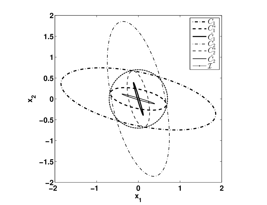
Finally, the first branch of the proof considers $I\wedge\neg C_{1}$; this contains the set of initial states not in $C_{1}$. These can now be addressed by the second forward invariant cut (set $C_{2}$) following a symmetric argument as above. After applying the second cut $C_{2}$, the first branch has an empty antecedent ($I\wedge\neg C_{1}\wedge\neg C_{2}$ is empty), i.e., the proof has accounted for all initial states, which closes the proof. The sets we have discussed are shown in Figure 3.

The system dynamics and parameters were derived from a published model [15] and then simplified, as in [17]. The model consists of a simplified version of the physics of engine subsystems responsible for air intake and A/F ratio measurement, along with a computer control system tasked with regulating the A/F ratio. The objective of the controller is to maintain the A/F ratio within 10% of the nominal operating conditions. The experiment that we model involves an engine connected to a dynamometer – a device that can control the speed of the engine and measure the output torque. In our setting, the dynamometer maintains the engine at a constant rotational velocity. The controller has two modes of operation: (1) a $\mathit{recovery}$ mode, which controls fuel in an open-loop manner, i.e., with only feedforward control action, where the system runs for at most $8$ms, and (2) a normal run mode, which uses feedback control to regulate the A/F ratio.

The controller measures both the air flow through the air-intake manifold, which it uses to estimate the air pressure in the manifold, and the oxygen content of the exhaust gas, which it uses to compute the A/F ratio. The $\mathit{recovery}$ mode represents the behavior of the controller when recovering from a sensor fault (e.g., aberrant sensor readings, environmental conditions that cause suspicion of the sensor readings). During the $\mathit{recovery}$ mode, the controller has no access to oxygen sensor measurements and so must operate in a feedforward manner (i.e., using only the manifold air flow rate). The normal mode is the typical mode of operation, where the oxygen sensor measurements are used to do feedback control.

Model 3 is a hybrid program representing this system. The ODEs representing the continuous dynamics in each mode and the model parameters are presented in the Appendix. The state variables $\hat{p},\hat{r},\hat{p}_{est}$, and $\hat{i}$ represent the manifold pressure, the ratio between actual air-fuel ratio and the stoichiometric value, the controller estimate of the manifold pressure, and the internal state of the PI controller; these variables have all been translated so that the equilibrium point coincides with the origin. In the $\mathit{recovery}$ mode, the continuous-time state $\mathbf{x}$ is the tuple $(\hat{p},\hat{r},\hat{p}_{est},\hat{i},\tau)$. The additional state variable in the $\mathit{recovery}$ mode represents the state of a timer that evolves according to the ODE $\dot{\tau}=1$. In the $\mathit{normal}$ mode, the state is given by $(\hat{p},\hat{r},\hat{p}_{est},\hat{i})$.

We assume the system is within $1.0\%$ of the nominal value at the initialization of the $\mathit{recovery}$ mode. This represents the case where the system was previously in a mode of operation that accurately regulated the A/F ratio to the desired setpoint. A domain of interest for the state variables is given by $\|\mathbf{x}\|_{\infty}<0.2$.

In previous work [17], the authors had established a forward invariant set for the $\mathit{normal}$ mode of operation using a barrier certificate formulation. The authors formulated the barrier certificate using simulation-guided techniques to obtain a candidate Lyapunov function $V$ and a number $\ell$ to propose a barrier function of the form $B(\mathbf{x})=V(\mathbf{x})-\ell$. Here, $V(\mathbf{x})$ = $\mathbf{z}^{T}P\mathbf{z}$, and $\mathbf{z}$ is a vector of all monomials of degree $\leq 2$ of the state variables $\hat{p}$, $\hat{r}$, $\hat{p}_{est}$ and $\hat{i}$. Note that $\mathbf{z}$ thus contains $14$ monomials, and $P$ is a $14\mathrm{x}14$ matrix. We omit the resulting $P$ matrix for brevity.

We use the set enclosed by the barrier function to formulate the forward invariant cut

Application of the forward invariant cut inference rule (6), generates three proof obligations that KeYmaera has to discharge.

In order to discharge the obligation for the program $\mathtt{m}_{2}$, we first perform some trivial simplifications with KeYmaera that leaves us with the following proof goal:

To discharge (20), we can use the barrier certificate rule shown in (21) that we have added to KeYmaera’s proof calculus.

where $H$ is the domain of evolution of the continuous dynamics. In our application of the barrier certificate rule, we substitute $\mathit{init}$ with $(B(\mathbf{x})\leq 0)$ and $\mathit{safe}$ with $(B(\mathbf{x})\leq 0)\wedge(M=\mathit{normal})$. The first and the third proof obligations in the barrier certificate rule are then trivially satisfied. For the remaining (middle) proof obligation KeYmaera uses the SMT solver dReal [11]. In particular, it asks dReal if the query $(B(\mathbf{x})=0)$ $\wedge$ $(\frac{\partial B}{\partial\mathbf{x}}\cdot f_{normal}(\mathbf{x})>-\epsilon)$ is unsatisfiable, where $\epsilon$ is a small positive number.

In order to discharge the proof obligation for $\mathtt{m}_{2}$, $\mathtt{s}_{\{1,2\}\mapsto fail}$, KeYmaera needs to show that if $B(\mathbf{x})<0$ holds, either of these programs cannot invalidate $C$ by transitioning to mode $fail$. It proves this by showing that the set $B(\mathbf{x})<0$ is a subset of the safe set using dReal.

To prove this obligation, we use the lemma that the set $C1$ is an invariant for all states remaining in $I\wedge\neg C$ . This is a bounded-time invariant certificate.

Here $S_{reach}$ is an overapproximation of reachable sets by using upper and lower bounds on $\dot{p}$ and $\dot{r}$ computed using dReal. The proof for this branch continues using standard KeYmaera deduction procedures. There is one additional barrier certificate application to show that the normal mode, when starting from this set, lands within the barrier certificate and therefore also respects this invariant. This requires a derivative negativity argument, which KeYmaera again handles via an external dReal query.

References

- [1] Abraham-Mumm, E., Hannemann, U., Steffen, M.: Verification of hybrid systems: formalization and proof rules in pvs. In: Engineering of Complex Computer Systems, 2001. Proceedings. Seventh IEEE International Conference on. pp. 48–57 (2001)
- [2] Abraham-Mumm, E., Hannemann, U., Steffen, M.: Assertion-based analysis of hybrid systems with pvs. In: Moreno-Diaz, R., Buchberger, B., Luis Freire, J. (eds.) Computer Aided Systems Theory, EUROCAST 2001, Lecture Notes in Computer Science, vol. 2178, pp. 94–109. Springer Berlin Heidelberg (2001), http://dx.doi.org/10.1007/3-540-45654-6_8
- [3] Beckert, B., Hähnle, R., Schmitt, P.H.: Verification of object-oriented software: The KeY approach. Springer-Verlag (2007)
- [4] Boyd, S., Ghaoui, L.E., Feron, E., Balakrishnan, V.: Linear Matrix Inequalities in System and Control Theory, vol. 15. SIAM (1994)
- [5] Branicky, M.S.: Stability of switched and hybrid systems. In: Decision and Control, 1994., Proceedings of the 33rd IEEE Conference on. vol. 4, pp. 3498–3503. IEEE (1994)
- [6] Chen, X., Abraham, E., Sankaranarayanan, S.: Flow*: An Analyzer for Non-Linear Hybrid Systems. In: CAV (2013)
- [7] Craig, W.: Three uses of the Herbrand-Gentzen theorem in relating model theory and proof theory. J. Sym. Logic 3, 269–285 (1957)
- [8] Dimitrova, R., Majumdar, R.: Deductive control synthesis for alternating-time logics. In: Proc. of the International Conference on Embedded Software. p. 14 (2014)
- [9] Frehse, G.: PHAVer: Algorithmic verification of hybrid systems past HyTech. STTT 10(3), 263–279 (2008)
- [10] Frehse, G., Le Guernic, C., Donzé, A., Cotton, S., Ray, R., Lebeltel, O., Ripado, R., Girard, A., Dang, T., Maler, O.: SpaceEx: Scalable verification of hybrid systems. In: CAV. pp. 379–395 (2011)
- [11] Gao, S., Avigad, J., Clarke, E.M.: -complete decision procedures for satisfiability over the reals. In: J. Automated Reasoning. pp. 286–300 (2012)
- [12] Gentzen, G.: Untersuchungen über das logische Schließen I,II. Mathematische Zeitschrift 39(2), 39(3): 176–210, 405–431 (1935)
- [13] Henzinger, T.A., Jhala, R., Majumdar, R., Sutre, G.: Lazy abstraction. In: ACM SIGPLAN Notices. vol. 37, pp. 58–70 (2002)
- [14] Henzinger, T.A., Kopke, P.W., Puri, A., Varaiya, P.: What’s Decidable about Hybrid Automata? JCSS 57(1), 94 – 124 (1998)
- [15] Jin, X., Deshmukh, J.V., Kapinski, J., Ueda, K., Butts, K.: Powertrain Control Verification Benchmark. In: Hybrid Systems: Computation and Control (2014)
- [16] Johansson, M., Rantzer, A.: Computation of piecewise quadratic Lyapunov functions for hybrid systems. IEEE Tran. on Automatic Control 43(4), 555–559 (1998)
- [17] Kapinski, J., Deshmukh, J.V., Sankaranarayanan, S., Aréchiga, N.: Simulation-guided Lyapunov analysis for hybrid dynamical systems. In: Hybrid Systems: Computation and Control (2014)
- [18] Kapinski, J., Krogh, B.H.: Verifying asymptotic bounds for discrete-time sliding mode systems with disturbance inputs. In: ACC. vol. 3, pp. 2852–2857 (2004)
- [19] Khalil, H.K.: Nonlinear Systems. Prentice Hall (2002)
- [20] McMillan, K.L.: Lazy abstraction with interpolants. In: Computer Aided Verification. pp. 123–136 (2006)
- [21] Meiss, J.D.: Differential Dynamical Systems (Monographs on Mathematical Modeling and Computation). SIAM (2007)
- [22] Parrilo, P.A.: Structured Semidefinite Programs and Semialgebraic Geometry Methods in Robustness and Optimization. Ph.D. thesis, California Institute of Technology (2000)
- [23] Platzer, A.: Logical Analysis of Hybrid Systems. Springer (2010)
- [24] Platzer, A.: The structure of differential invariants and differential cut elimination. Logical Methods in Computer Science 8(4), 1–38 (2012)
- [25] Platzer, A., Clarke, E.M.: Computing differential invariants of hybrid systems as fixedpoints. In: Computer Aided Verification (2008)
- [26] Prajna, S.: Optimization-based methods for nonlinear and hybrid systems verification. Ph.D. thesis, California Institute of Technology, Caltech, Pasadena, CA, USA (2005)
- [27] Prajna, S.: Barrier certificates for nonlinear model validation. Automatica 42(1), 117–126 (2006)
- [28] Prajna, S., Jadbabaie, A.: Safety Verification of Hybrid Systems Using Barrier Certificates. In: Hybrid Systems: Computation and Control. pp. 477–492 (2004)
- [29] Topcu, U., Seiler, P., Packard, A.: Local stability analysis using simulations and sum-of-squares programming. Automatica 44, 2669–2675 (2008)
- [30] Vandenberghe, L., Boyd, S.: Semidefinite Programming. SIAM Review 38(1), 49–95 (March 1996)
Appendix
A Semantics of d
We follow the development of [23], Chapter 2. Symbols in d are classified into three different syntactic categories, depending on their role.
- 1.
represents a set of rigid symbols that cannot change their value, such as ;
- 2.
represents a set of flexible symbols, also called state variables, which change their value as the system evolves;
- 3.
represents a set of logical variables, which do not change as the system evolves, but can be quantified over universally and existentially; they often serve the role of parameters.
An interpretation is a function that associates functions and relations over the reals to function and relation symbols in . The standard arithmetic operators and relations symbols, such as , , , are interpreted as usual.A state is a map , which maps a real value to each state variable. An assignment is a map that prescribes the value of the logical variables. Note that the value of the logical variables does not depend on the state.
A state variable is a term, and a logical variable is also a term. The result of applying a function of arity to terms is also a term. Nothing else is a term.
Definition 1 (Valuation of terms ([23], Defn. 2.5)).
The valuation of terms with respect to interpretation , assignment , and state is defined as
if is a logical variable.
if is a state variable.
if is a function of arity and are terms.
The notation represents the function that agrees with except for the interpretation of , where it takes the value . The notation denotes the modification of a state , that agrees with everywhere except the interpretation of the state variable , where it takes the value .
Definition 2 (Valuation of d formulas ([23], Defn. 2.6).
The valuation of formulas with respect to interpretation , assignment , and state is defined as
.
iff and .
iff or .
- 4.
iff .
- 5.
- 6.
iff for all .
- 7.
iff for some .
- 8.
iff for all states for which the transition relation (defined below) satisfies .
- 9.
iff for some state such that the transition relation satisfies .
We now define the transition semantics of hybrid programs. We already saw a glimpse of it in the definition of valuation of formulas, since the formulas and programs of d are constructed coinductively.
Definition 3 (Transition semantics of hybrid programs ([23], Defn. 2.7)).
The valuation of a hybrid program , denoted is a transition relation on states that specifies which states are reachable from a state under the program , and is defined inductively as follows.
iff the state equals the state obtained by modification of as .
iff there is a flow of some duration from to along the differential equations that always respects the invariant .
iff there is a sequence of states states with , , and such that for each .
B Soundness proof for forward invariant cut
Fix an interpretation and an assignment . From semantics of the first premise, if and , then . From the semantics of the second premise, if , then From the semantics of the third premise, if and , and is such that , then . This is equivalent to saying that for any such that there is a sequence of states , with and , , and for each , it is the case that .
The proof is to show by induction that any state reachable by from in executions of must be contained in .
For the base case, let . Then given , the only reachable state by a sequence of length zero is itself. If , then by semantics of the second premise. If , we have that by a chain of length zero, so that by semantics of the third premise, .
As an inductive hypothesis, suppose that for every reachable by a chain of length , (i.e., there exists with and such that , for . Now choose any state such that there is a chain of length , with and , such that , for ).
First suppose that . Then by semantics of the first premise, , and then by semantics of the second premise. On the other hand, suppose . We claim that for all , . To see this, note that if for some , then by semantics of the first premise, which would contradict our assumption on . Then we have that for all . By semantics of the third premise, it follows that . This establishes the theorem.
C System dynamics for the Engine Fuel Control Model
We now present the model parameters and the ODEs for the Engine Fuel Control model. Figure 4 details the equations for the mode, and Fig. 5 provides the dynamic equations for the mode. In the figures, , , , and .