Type I and Type II Bayesian Methods for Sparse Signal Recovery using Scale Mixtures
Abstract
In this paper, we propose a generalized scale mixture family of distributions, namely the Power Exponential Scale Mixture (PESM) family, to model the sparsity inducing priors currently in use for sparse signal recovery (SSR). We show that the successful and popular methods such as LASSO, Reweighted and Reweighted methods can be formulated in an unified manner in a maximum a posteriori (MAP) or Type I Bayesian framework using an appropriate member of the PESM family as the sparsity inducing prior. In addition, exploiting the natural hierarchical framework induced by the PESM family, we utilize these priors in a Type II framework and develop the corresponding EM based estimation algorithms. Some insight into the differences between Type I and Type II methods is provided and of particular interest in the algorithmic development is the Type II variant of the popular and successful reweighted method. Extensive empirical results are provided and they show that the Type II methods exhibit better support recovery than the corresponding Type I methods.
Index Terms:
Sparse Bayesian Learning, LASSO, Reweighted , Reweighted , Gaussian Scale MixtureI Introduction
Sparse signal recovery (SSR), i.e, finding sparse signal representations from overcomplete dictionaries, has become a very active research area in recent times because of its wide range engineering applications and interesting theoretical nature [1, 2, 3, 4].
I-A Problem Formulation
The SSR problem involves solving an under-determined system of equations where vector is the measurement vector and is the overcomplete dictionary, where and it is assumed that are often formed from a physically meaningful model and the vector is the vector of interest. As the system has fewer equations than unknowns, it can have infinitely many solutions and thus additional information is needed to identify which of these candidate solutions is indeed the appropriate one for the problem at hand. In the SSR problem, it will be assumed that the solution of interest is sparse, i.e. most of the entries are zero. Ideally one can recover the optimal sparsest solution by solving the following optimization problem [4],
| (1) |
where is a measure of the support of In practice, measurements are generally corrupted by noise, which motivates the following modified optimization problem:
| (2) |
where, is related to the measurement noise variance.
However, the above optimization problem is not convex and is known to be NP-hard. For computational tractability, the original penalty factor is often approximated by a suitable surrogate leading to the optimization problem
| (3) |
Different choices of the penalty factor also referred to here as diversity measure, lead to different SSR algorithms [5, 6, 7, 8], and it has been shown that the choice of a strictly concave penalty factor on the positive orthant leads to a objective function with local minima being sparse and sparsest solution as a global minimum under some conditions [9]. Majorization-Minimization [10] can be employed to solve this optimization problem for such penalty functions, and this has led to the development of useful and effective reweighted norm minimization algorithms. Typically, and norms are selected because of their convex nature and the later because of the closed form solution at each iteration.
I-B Related Literature
Minimizing diversity measures to recover the sparse representations has been a popular algorithm exploration avenue. In this framework, the SSR problem formulation can also be viewed as a regularization approach to signal reconstruction. A popular approach among this class is the norm minimization based methods. leads to a tractable and computationally attractive convex optimization problem and the very well known approaches such as Basis Pursuit, LASSO are based on the framework [11, 12]. Other than the convexity property, based approaches have been supported by theoretical guarantees of exact recovery given some conditions on the overcomplete dictionary [8], which makes these approaches attractive options. The recently proposed reweighted and norm minimization approaches [6, 5, 13] have empirically shown superior recovery performance over minimization and are considered in this work.
In addition to the regularization framework, another options for SSR algorithm development is the Bayesian framework [14, 15, 16, 17, 18, 19, 20]. In a Bayesian framework, the sparsity constraint is incorporated by choosing a suitable sparse prior on the coefficient vector . In a Bayesian setting, there are two popular avenues for algorithm development: a Type I MAP based approach, and a Type II Evidence Maximization approach involving a Hierarchical model. Most of the approaches discussed above, based on (3), can be interpreted and cast in a suitable Type I framework. A Type II framework has been considered in [21, 15], where a Relevance Vector Machine is adapted to the problem at hand. In [22, 23, 24] a Type II optimization problem has been transformed into a Type I problem by employing a suitable penalty function and reweighted norm minimization algorithm is developed to solve the resulting optimization problem. Following the Type II framework, a Laplacian prior which corresponds to norm minimization can also be represented in a Hierarchy using a Gaussian Scale Mixture (GSM) representation [16, 25]. In the statistics community, the well known Bayesian Lasso [26] also makes use of the equivalence of a hierarchical Gaussian-Exponential prior to the Laplace prior, and conducts a fully Bayesian inference (via Markov chain Monte Carlo or MCMC sampling algorithms). Demi-Bayesian Lasso [27] solves the same problem using a Type II approach. It has been shown empirically that a Type II methods performs consistently better than Type I, i.e the MAP estimation approach, and theoretical analysis in support for this superiority has recently begun to appear. However, much remains to be done and this work is an attempt in this direction. In [28], the two different frameworks are analyzed in a generalized Hierarchical Bayesian setting which motivates us to analyze these two frameworks for the specific SSR problem to gather additional insights by exploiting domain knowledge. In [29], Type I and Type II frameworks for SSR were introduced using two forms of density representation, a convex representation and a GSM representation, to provide an unified treatment. We build on this work and employ a generalized scale mixture representation to establish connections and develop enhancements to popular SSR algorithms, as well as treat both and variants in an unified manner.
As mentioned above, a key ingredient behind the Type II methods is the Scale Mixture/Hierarchical representation of the super gaussian priors, which allows one to design efficient algorithms conveniently. Gaussian Scale Mixtures (GSM) [30, 31, 29] and Laplacian Scale mixtures (LSM) [32] have been studied before in the context of sparsity. In this work we discuss a more general Scale Mixture framework, the Power Exponential Scale Mixture (PESM) family, for SSR algorithm development. The PESM representation includes the popular GSM and LSM as special cases and provides a mechanism to provide a unified view of the popular and frameworks currently employed. This work will emphasize the generalized t (GT) distribution family of priors, a member of PESM, since it has a wide range of tail shapes, and also includes the heavy tailed super gaussian distributions. GT family of distributions have been mentioned in statistics literatures for design of robust regressors for several financial modeling tasks, where the heavy tail nature of GT helps to model the outliers [33, 34].
I-C Contributions of the Paper
- •
We discuss a generalized scale mixture framework, the power exponential scale mixture (PESM) family, and show how many of the super gaussian densities used in practice can be represented using this framework.
- •
We summarize two types of Bayesian frameworks, i.e. Type I and Type II for SSR in detail, along with providing connections to traditional norm minimization approaches by suitable choice of sparse prior distributions. Of particular importance is the treatment of the diversity measure used in connection with the reweighted algorithm as well as an unified treatment of both and based approaches.
- •
We formulate and unify three well known diversity minimization based SSR algorithms in the PESM framework and derive the Type I and Type II versions of them. Of particular interest is the Type II counterpart of the reweighted algorithm [5].
- •
We analyze the difference between Type I and Type II inference procedures and our analysis shows the fundamental difference between these two frameworks and also helps to understand a potential reason for the empirical superiority of Type II methods over Type I.
- •
Extensive empirical experimentation results are presented to support the superiority claim of Type II methods over their Type I counterpart.
I-D Article Organization
The rest of the paper is organized as follows. In Section II-A, a generalized scale mixture representation, the Power Exponential Scale Mixtures (PESM) family, is presented which are of main importance to design Bayesian methods for SSR. In Section III we discuss Type I/MAP algorithms for SSR and derive a unified inference procedure and provide connection with three well known SSR algorithms. In Section IV we discuss Type II framework for SSR along with analyzing the fundamental difference between Type I and Type II algorithms. The EM based inference procedure for Type II algorithms to estimate the coefficient vector and the hyperparameters is also developed which includes the counterpart to the popular reweighted method. We present experimental results of the proposed algorithms in Section V in different settings and finally conclusions are presented in Section VI.
II Scale Mixture Distributions
Scale mixture distributions namely Gaussian Scale mixtures (GSM) and Laplacian Scale mixtures (LSM) have gained lot of attention in recent years because of their ability to represent complex heavy tailed super gaussian distributions in a simple hierarchical manner [30, 31, 29, 32]. In the statistics community, robustness has been the major reason for the use of scale mixtures. In regression analysis, the method of least squares often fails because of the outliers in the data. The need to model the outliers motivates the use of heavy tailed distribution.
II-A Power Exponential Scale Mixture (PESM) distribution
In this work, a more general Power Exponential Scale Mixture (PESM) distribution, which is a generalization of GSM and LSM, is presented. The PESM representation is then used to model the prior sparse distribution over the vector and for sparse signal recovery algorithm development.
Power exponential (PE) distributions were first introduced by Box and Tiao (1962) in the context of robust regression to deal with non-normality. PE distribution is symmetric about the origin and a zero mean PE distribution has the following parameterized form:
| (4) |
It is evident from the above given form, that results in the normal distribution, whereas connects to the well known Double exponential or Laplacian distribution. leads to distribution with heavier tails than the Gaussian distribution.

PESM family of distributions refer to distributions that can be represented as follows:
| (5) |
Choice of distributional parameter along with different suitable mixing densities, i.e will lead to different distributions including the super gaussian distributions. Because of the scale mixture representation, the generation of the random variable can be viewed in a hierarchy, i.e. generate using followed by generating using . The framework allows for dealing with complicated models in a simple manner and is indispensable as we move towards complex problems with structure.
As special cases, the choice of leads to Gaussian Scale Mixtures (GSM) which has been very popular in the literature, and leads to the Laplacian Scale Mixtures (LSM). Interestingly, a Laplacian distribution can be represented as a GSM with exponential mixing density i.e. where is the unit step function [16]. More explicitly,
| (6) |
This means, any LSM can also be represented as a GSM with an extra layer of hierarchy. This will play an important role in the SSR algorithm development. This fact also leads to the observation of the relationship between the different scale mixture families as depicted in Figure 1.
II-B An example of PESM: Generalized t Distribution
In this example, we will consider an inverse generalized gamma (GG) distribution as our mixing density in the hierarchical representation (5) for the PESM family. It leads to a generalized t distribution which is a superset of all the sparse distributions that have been used in practice in several recent works, e.g. Generalized double Pareto (GDP), Laplacian and Student-t distributions, among others.
The Generalized t Distribution has the form:
| (7) |
Where is the normalization constant, and are the shape parameters and is the scale parameter. Interestingly, and provide the flexibility to represent different tail behavior using this distribution. Larger values of and correspond to thin tailed distributions whereas smaller values of and are associated with heavy tailed distributions.
As mentioned above, the GT distribution family can be represented in PESM framework using where,
| (8) |
Interesting special case of note is which leads to a student t distribution, a prior that has been used in the popular Sparse Bayesian Learning (SBL)/Relevance Vector Machine (RVM) work and can be decomposed as a Gaussian Scale mixture with inverse Gamma as the mixing density. Employing leads to a Generalized Double Pareto distribution (GDP) discussed in [35] which can be represented as a scale mixture of Laplacian following equation 5.
In Table I, we summarize some special cases that have been used for SSR that arise by different choices of the shape parameters of GT, i.e. and
Among Scale Mixtures, GSM in particular has gained a lot of interest over the years in the literature and the proposed PESM framework is an interesting generalization for SSR purposes. As shown in [29], GSM can only be used to represent supergaussian densities, i.e. distributions with positive kurtosis whereas PESM representation can also be used for subgaussian densities along with supergaussian densities. One example is the previously discussed generalized t distribution, which becomes a thin tailed subgaussian distribution for (, ). Moreover, for the purposes of the SSR work, the general PESM allows one to treat both the LSM and GSM in a unified manner thereby enabling treatment of and based algorithms in a unified manner.
III B-SSR: Type I
Type I inference corresponds to standard MAP estimation technique in B-SSR. In this section we review the Type I framework and derive a Type I algorithm using PESM as the sparse prior. Then we specialize the result using the Generalized t distribution as the sparse prior and also show that the generalized algorithm reduces to well known SSR algorithms.
III-A Background on MAP Estimation (Type I methods)
Having chosen a sparsity enforcing distribution thereby allowing one to narrow the space of candidate solutions in a manner consistent with application-specific assumptions, a maximum a posteriori (MAP) estimator of is then obtained as (Type I estimation)
| (9) |
Using the Gaussian noise assumption, and a separable prior distribution , the MAP estimate is obtained by minimizing
| (10) |
where is determined by Incorporating sparsity by enforcing a sparse (supergaussian) distribution as the prior, reduces to choosing . It has been shown that which is symmetric, concave and nondecreasing functions on are useful choices in this context [36]. Now, as discussed above, many of these sparse priors can be represented in a hierarchy and belong to the PESM family.
In order to contrast with the Type II formulation to follow, with the PESM representation one can revisit the equation (9) and note that Type I involves integrating out the hyperparameter .
| (11) |
| q | p | Prior Distribution | Penalty Function | SSR Algorithm |
|---|---|---|---|---|
| 2 | Normal | Ridge Regression | ||
| 1 | Laplacian | LASSO | ||
| (degrees of freedom) | 2 | Student t distribution | Reweighted (Chartrand’s) | |
| (shape parameter) | 1 | Generalized Double Pareto | Reweighted (Candes’s) |
III-B Unified Type I Inference Procedure
In this section we derive the EM inference procedure for the PESM family in the Type I framework, i.e, we find the MAP estimate of where a PESM has been employed for the sparsity inducing prior . Because of the separable prior, the have an independent scale mixture representation,
| (12) |
For MAP estimation of we treat the ’s as hidden variables and employ an EM algorithm. The complete data log-likelihood can be written as,
| (13) |
To formulate the Q function, we need to find the conditional expectation of the complete data log-likelihood with respect to posterior of the hidden variables which reduces to by virtue of the Markovian property induced by the hierarchy, i.e. Since in the M step we need to maximize the Q function with respect to , we are only concerned with the first two terms in (13) and only the second term has dependencies on . This is the only term we need to be concerned with during the E-step. Now from the scale mixture decomposition and considering the ith component of ,
| (14) |
Hence, for determining the Q function we need the following conditional expectation, .
To compute the concerned expectation we will use the following trick. Differentiating inside the integral of the marginal ,
| (15) |
Hence,
| (16) |
and enables determining the Q function. Then the M step reduces to,
| (17) |
Where is the variance of the measurement noise and .
Following the traditional path of EM, the algorithm is an iterative one, i.e, in the E step the weights are computed and in the M step a weighted norm minimization is solved. This alternate procedure is carried out iteratively till convergence.
III-C Special cases of Type I using Generalized t distribution
In this section we specialize the derived unified Type I EM algorithm with the generalized t distribution as . We can write where,
| (18) |
Thus,
| (19) |
Substituting the value of we get,
| (20) |
So the M step will become,
| (21) |
Where is the variance of the measurement noise and .
In following subsections we will show how with specific choices of the distribution parameters of the generalized t, we can derive well known Type I (MAP estimation) based SSR algorithms.
III-C1 LASSO (-minimization) [11]
Interestingly we see from Table I that for specific values of the shape parameters ( and ), a generalized t distribution can be used to represent a double exponential or Laplacian distribution. Now to relate with the unified Type I MAP estimation inference procedure, taking the limit as and in (20), we get . Hence in the M step we are just solving a penalized regression once as the weights are not changing over iterations, which is essentially the LASSO algorithm.
III-C2 Reweighted -minimization (Candes et al [5])
The popular reweighted -minimization (Candes et al [5]) is a special case of the MAP estimation approach using a generalized t distribution as sparse prior.
Selecting the parameters of the generalized t as follows; , one obtains,
| (22) |
which when substituted in equation (10), results in the following cost function,
| (23) |
In [5], the above mentioned cost function is optimized using a MM approach. Now substituting the distribution parameters in equation (20), the weights reduce to . These are the same weights obtained in [5] via a MM method and in Equation (21) results in a weighted minimization problem with the weights being a function of the previous estimate. This special case of GT has been also called the Generalized Double Pareto (GDP) distribution in the literature [35].
Following the scale mixture decomposition of the GT distribution, as shown in Equation (5), since we can represent the prior as a Laplacian Scale Mixture.
| (24) |
where . This observation is summarized in the following lemma.
Lemma III.1
Let , , then the resulting marginal density for is .
III-C3 Reweighted -minimization ([6, 13])
Another popular SSR algorithm, the reweighted minimization can also be represented in a Bayesian Type I setting by employing a Student t distribution with degree of freedom This heavytailed sparse prior is again a special case of the generalized t distribution as shown in the table.
| (25) |
The nature of the tail of the student t distribution is controlled by degrees of freedom parameter and smaller values of correspond to heavier tails. The associated diversity penalty factor is given by . For a Type I inference procedure, we can utilize the unified approach discussed above in Section III-C and substitute the shape and scale parameters of the generalized t distribution in Equation (20) to obtain, Since Equation (21) leads to the reweighted minimization algorithm as discussed in [6].
IV B-SSR: Type II (Evidence Maximization)
The success of Type II approaches like SBL for SSR problems motivate the Type II approach for the general PESM family. As special cases, the three Type I algorithms discussed in Section III-C are explored in the Type II setting. We also analyze the difference between a Type I algorithm and its Type II counterpart which provides insights into the reasons for superior recovery performance of Type II methods.
In a Type II procedure, instead of integrating out the hypeparameters , we estimate them using an evidence maximization method, i.e.
| (26) |
The evidence framework integrates over the coefficient vector to obtain the evidence . This evidence is weighted by the hyperprior and maximized over . Once is obtained, the relevant posterior is approximated, often as and the mean of the approximated posterior is used as a point estimate. Sparsity is achieved by many of the being zero [21, 22, 23].
IV-A Unified Type II EM algorithm
To solve the above mentioned optimization problem, we again employ the EM algorithm this time by treating as the hidden variable. As in Section III-B, we assume a sparse prior from the PESM family has been utilized and that the measurement noise is Gaussian with variance .
Hence the Q function has the form,
| (27) |
Since in the M step we are only concerned with the terms involving , examining them reveals that the E-step requires the computation of the following conditional expectation
| (28) |
In the M step we will maximize the Q function with respect to to find the update rules. To illustrate, if we consider a non informative hyperprior, i.e, ,
| (29) |
Taking the derivative of the Q function w.r.t and setting it to zero results in,
| (30) |
Since the E step requires the computation of the conditional expectation given by Equation (28), we can either look for a closed form solution or revert to the MCMC technique [26]. We will examine this further for some special cases later.
IV-B Difference between Type I and Type II inference methods
Type I and Type II provide two different approaches to solving the SSR problem. Hence it is important to understand the theoretical differences between the two inference procedures to identify their suitability for SSR. In [37], the authors provide evidence for SBL, using a variational approximation to the prior that Type II methods attempt to approximate the true posterior If the true posterior distribution has a skewed peak, then the type I estimate (MAP of ) is not a good representative of the whole posterior. By trying to approximate the true posterior mass, Type II methods are likely to provide a better estimate. Similar discussion of Type II desirability is provided in [28] in the context of general Bayesian inferencing. We revisit the issue and attempt to corroborate this by exploiting specific attributes of the SSR problem. We first manipulate the Type II objective as shown below.
| (31) |
Lets assume that is the solution of Equation (26). It will be sparse for specific choice of as shown in [22, 23].
Now, let be the index of non zero entries and be the index of zero entries. So, we can say .
| (32) |
is a normal distribution with mean zero and variance . Hence when , becomes a dirac delta function, i.e. .
Using the properties of dirac delta functions inside the integration, we obtain
| (33) |
Hence from this analysis, we see that we are evaluating a weighted integral of the true posterior over the subspaces spanned by the non zero indexes. This shows that in the evidence maximization framework instead of looking for the mode of the true posterior , we approximate the true posterior by where is obtained by maximizing the true posterior mass over the subspaces spanned by the non zero indexes. This is in contrast to Type I methods that seek the mode of the true posterior and use that as the point estimate of the desired coefficients.
Another favorable aspect of the Type II framework is that it inherits the robustness property of a Hierarchical Bayesian modeling framework. It has been shown extensively in the statistics literature [38, 39, 40], that the posterior of a hyperparameter, i.e, is less affected by the wrong choices of prior than the posterior of the parameter . In other words, parameters that are deeper in the hierarchy have less effect on the inference procedure, which allows us to be less concerned about the choice of . Another virtue is that the hierarchical framework allows for parameter tying and this can greatly reduce the search space for Type II methods by leading to an optimization problem with fewer parameters. This is more evident for problems like the MMV and block sparsity problem [41, 42, 43].
IV-C Special case of Unified Type II with different choices of
As discussed above for the unified Type II approach our concerned posterior is . For a point estimate of we will use the mean of the posterior, . Now the posterior could be computed as,
| (34) |
The challenge is proper normalization and tractability of the computation of the mean. For the EM algorithm to be successfully implemented, one must also be able to carry out the E-step, Equation (28). We now explore this for some specific PESM family members.
IV-C1 Choice of
Choice of corresponds to Gaussian Scale Mixture, and is very tractable. The GSM based Type II methods have been extensively studied [15, 21, 37] and so we keep the discussion brief. This choice (in Equation (34)) leads to a Gaussian posterior given by
| (35) |
where
| (36) |
| (37) |
and . The EM algorithm can also be readily carried out because the E-step requires the second moment which can be readily obtained using Equation (37). The estimate of in the M step and the updates of depend on the mixing density as shown in Equation (27) and can be readily carried out for the non-informative prior and for a reasonable large class of priors [29]. The true posterior can be approximated by a Gaussian distribution whose mean and covariance depend on the estimated hyperparameters. Now, for a point estimate of the coefficient vector, we will choose,
| (38) |
From Equation (36), one can see that is sparse if is sparse. To complete the discussion, we discuss the most popular of the Type II methods. In Relevance Vector Machine (Type II) [21], Tipping has shown that the ’true’ coefficient prior used in SBL actually follows a student t distribution (GSM with Gamma distribution as mixing density), and discusses in detail how the hierarchical formulation of this prior helps to realize the supergaussian nature. Hence we can see that the corresponding Type II formulation of Reweighted is SBL with a slight difference. In SBL is set to zero which gives us an improper prior which is sharply peaked at zero. But as discussed in previous literatures, in Type I version, i.e, in Reweighted increases the number of local minima and convergence to a sub optimal solution becomes more likely. Now to solve the M step for this case we will use the following PESM () formulation,
Lemma IV.1
Let , Then the resulting marginal density for is .
IV-C2 Choice of
With PESM reduces to a Laplacian Scale Mixture. To successfully carry out the EM algorithm, the E-step requires the computation of A closed form expression does not appear feasible and a more numerical approach may be required. Also, the concerned posterior (Equation 34) does not appear to have a simple closed form expression making final inferencing a challenge along with the computation of the mean for the point estimate. An efficient numerical approach needs to be developed and is left for future work.
In this work, we follow an alternate strategy and take advantage of the fact that the LSM family is contained within the GSM family. Since a Laplacian distribution can be written as a member of the GSM family (Equation 6) [16, 25], it will be possible to get a closed form posterior using a three layer hierarchy. We will illustrate this for the prior associated with Type I Reweighted -minimization approach and develop a Type II variant. The closed form posterior will be Gaussian and have the same form for the case of as shown in Equation (35). The only difference between and lies in the estimation of the hyperparameters.
Type II variant can also be derived and has been dealt with in previous work [16] and for sake of completeness the update rule is summarized in Table II along with other Type II algorithms. We will now derive the M step for the case of Type II Reweighted -minimization which can be followed in a straightforward manner for other cases including the variant.
We have shown in the discussion of Type I Reweighted that the concerned prior in a Bayesian setting is a Laplacian Scale mixture. This prior can be represented in a 3 layer hierarchy involving a GSM representation for the Laplacian density as summarized below.
Lemma IV.2
Let , and where . Then the resulting marginal density for is .

Fig. 3 compares two corresponding densities, and Laplace distribution with . It is evident from this figure that the Laplace prior has relatively light tails which contributes to the problem of over-shrinking of the large coefficients. On the other hand, the generalized t distribution has relatively heavier tails and a peak at zero which promotes zero coefficients. This is another reason of the superior recovery performance of Reweighted -minimization over the LASSO, i.e. -minimization, approach.

| Type II algorithm | Mixing Density | Update Rules |
|---|---|---|
| Type II | , | |
| Type II Re- (Candes) | , | , |
| Type II Re- (Chartrand) |
Now, for estimation of hyperparameters and in the three layer hierarchy, an EM algorithm will be developed. As in Section IV-A, using as the complete data, maximizing the conditional expectation of the complete data log likelihood involves maximizing,
| (39) |
In the E step, for iteration we only need to compute the second moment which is straightforward because of the GSM representation of the Laplacian, i.e.
| (40) |
In the M step, the Q function is maximized with respect to the hyperparameters, and .
| (41) |
Now using the E step and only retaining the terms that involve and we obtain,
| (42) |
In the M step, taking the derivative of the Q function w.r.t and and setting to zero results in.
| (43) |
Solving this quadratic equation we obtain,
| (44) |
Similarly,
| (45) |
Hence,
| (46) |
We can also estimate the measurement noise variance by maximizing the above Q function as shown in [21]. In this work, for simplicity, we will assume that the SNR of the environment is known to us before hand. We can also employ a fixed point optimization technique as shown in [21] to estimate the hyperparameters.
After convergence, one finds that most of the i.e. the variance of the normal distribution are driven to zero, which makes the associated coefficient zero and prunes it out from the model.

V Numerical Experiments
In this section we present a set of experiments to evaluate and compare the Type II/Hierarchical framework based methods with those based on regularization framework, i.e. Type I methods (MAP estimation), for the task of sparse signal recovery. The experimental setup used is quite standard and has been used widely in the SSR literatures.
V-A Problem Specification
The measurement vector is generated using a dictionary , whose elements are generated from a i.i.d normal distribution with mean=0 and variance=1. A sparse signal of length 250 is generated such that . The support, i.e. the location of the k nonzero elements, is chosen randomly, and the values are chosen from three different distributions:
- (I)
Uniform random spikes. (Sub-Gaussian)
- (II)
Zero mean unit variance Gaussian.
- (III)
Student t distribution with degrees of freedom . (Super-Gaussian)
The synthetic measurements are generated using . The generated measurements and the dictionary are then provided as input to the algorithms. The estimated coefficients are compared with the original that has been used to generate the measurement. For a single instance, the method is credited with a successful recovery if the estimate satisfies,
| (47) |
500 trials are conducted for various fixed combinations of k, i.e. the number of non zero coefficients, and the probability of successful recovery is plotted with respect to k. As expected, the probability of successful recovery decreases as k, i.e. the cardinality of support, increases.
V-B Recovery Performance
V-B1 Competing Algorithms
Since the main goal of our work is to compare the Type I algorithms with their Type I counterparts, we designed the Type II versions of three well known norm minimization based Type I algorithms and compare their performance. The algorithms in the study are:


V-B2 Performance Comparison
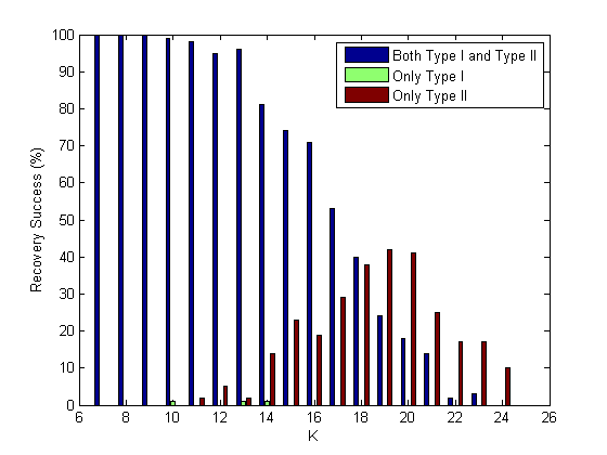
In Figure 6, the probability of successful recovery with increasing support cardinality is plotted for the case where the non zero coefficients are from a zero mean, unit variance, Gaussian distribution. It is evident from this plot that for all the algorithms, Type II versions outperform their Type I counterparts. This performance difference is significant in case of norm minimization. Type I Reweighted minimization approach works much better compared to other two Type I methods, and the reason being the heuristic update of , which helps it to get away from local minima. Hence, update in Reweighted (Type I) is absolutely necessary as we have found out for fixed this algorithm’s performance decreases significantly. Figure 4 shows this comparison for the Reweighted minimization (Candes et al) in detail. The figure indicates trials when both Type I and Type II method have been successful and when only one of them has been successful and it is evident that for high values of Type II outperforms Type I by a significant margin.
In Figure 7, the probability of successful recovery with increasing support cardinality is plotted where the non zero coefficients are generated from a student’s t distribution with degrees of freedom 3. Again, the empirical superiority of the Type II versions over their Type I counterparts is evident from Figure 7. Interesting point to note here, is the performance improvement of Type I and Type II version of Reweighted algorithm over the others is significant and the reason could be that assumed prior for the non zero coefficients and the true prior have the same tail behavior (student’s t) and are better matched.
Finally, we repeat the same set of experiments where the non zero coefficients follow a sub-gaussian distribution, i.e. Uniform random spikes, and the plot of the probability of successful recovery with increasing support cardinality is shown in Figure 8. Though Type II methods still outperform their Type I counterparts, the performance improvement is less significant compared to the previous two cases. The reason could be that, since the assumed priors are supergaussian, i.e. heavy tails, it is difficult to model the true prior, i.e. sub gaussian density, for the nonzero coefficients. In Figure 5, an instance of reconstruction is shown using along with the original signal. It is evident that both minimization (Type I) and Candes’s Reweighted minimization (Type I) fail, whereas Type II version of minimization recovers the original signal. For this instance, the other three SSR algorithms have also been successful in recovering the original signal.
VI Conclusion and Discussion
In this paper, we formulated the SSR problem from a Bayesian perspective and presented two different Bayesian frameworks which encompass all the well known recovery algorithms in practice. We presented a generalized scale mixture family : PESM, which is of prime importance for the design of Hierarchical Bayesian Recovery algorithms, i.e, Type II algorithms. The unified treatment of both and norm minimization based algorithms along with the design of Type II version of the Reweighted minimization algorithm are the main contributions of this work.
We also showed that, in a hierarchical Bayes framework instead of looking for a mode of the true posterior Type II methods actually try to find an approximate posterior such that the mass of the true posterior over the subspace spanned by non zero indexes is maximized. This leads to a better approximation of the true posterior, which is the reason behind the superior empirical results obtained using the Type II framework. Type II framework also enjoys the robustness property inherited because of its connection with Hierarchical Bayes which allows one to be less concerned about the choice of prior on the hyperparameters.
References
- [1] Yonina C Eldar and Gitta Kutyniok, Compressed sensing: theory and applications, Cambridge University Press, 2012.
- [2] Alfred M Bruckstein, David L Donoho, and Michael Elad, “From sparse solutions of systems of equations to sparse modeling of signals and images,” SIAM review, vol. 51, no. 1, pp. 34–81, 2009.
- [3] David L Donoho, “Compressed sensing,” Information Theory, IEEE Transactions on, vol. 52, no. 4, pp. 1289–1306, 2006.
- [4] Michael Elad, Sparse and redundant representations: from theory to applications in signal and image processing, Springer Science & Business Media, 2010.
- [5] Emmanuel J Candes, Michael B Wakin, and Stephen P Boyd, “Enhancing sparsity by reweighted ℓ 1 minimization,” Journal of Fourier analysis and applications, vol. 14, no. 5-6, pp. 877–905, 2008.
- [6] Rick Chartrand and Wotao Yin, “Iteratively reweighted algorithms for compressive sensing,” in Acoustics, speech and signal processing, 2008. ICASSP 2008. IEEE international conference on. IEEE, 2008, pp. 3869–3872.
- [7] Ingrid Daubechies, Ronald DeVore, Massimo Fornasier, and C Sinan Güntürk, “Iteratively reweighted least squares minimization for sparse recovery,” Communications on Pure and Applied Mathematics, vol. 63, no. 1, pp. 1–38, 2010.
- [8] David L Donoho and Michael Elad, “Optimally sparse representation in general (nonorthogonal) dictionaries via ℓ1 minimization,” Proceedings of the National Academy of Sciences, vol. 100, no. 5, pp. 2197–2202, 2003.
- [9] Bhaskar D Rao, Kjersti Engan, Shane F Cotter, Jason Palmer, and Kenneth Kreutz-Delgado, “Subset selection in noise based on diversity measure minimization,” Signal Processing, IEEE Transactions on, vol. 51, no. 3, pp. 760–770, 2003.
- [10] Mário AT Figueiredo, José M Bioucas-Dias, and Robert D Nowak, “Majorization–minimization algorithms for wavelet-based image restoration,” Image Processing, IEEE Transactions on, vol. 16, no. 12, pp. 2980–2991, 2007.
- [11] Robert Tibshirani, “Regression shrinkage and selection via the lasso,” Journal of the Royal Statistical Society. Series B (Methodological), pp. 267–288, 1996.
- [12] David L Donoho, “For most large underdetermined systems of linear equations the minimal -norm solution is also the sparsest solution,” Communications on pure and applied mathematics, vol. 59, no. 6, pp. 797–829, 2006.
- [13] Bhaskar D Rao and Kenneth Kreutz-Delgado, “An affine scaling methodology for best basis selection,” Signal Processing, IEEE Transactions on, vol. 47, no. 1, pp. 187–200, 1999.
- [14] Lihan He and Lawrence Carin, “Exploiting structure in wavelet-based bayesian compressive sensing,” Signal Processing, IEEE Transactions on, vol. 57, no. 9, pp. 3488–3497, 2009.
- [15] Shihao Ji, Ya Xue, and Lawrence Carin, “Bayesian compressive sensing,” Signal Processing, IEEE Transactions on, vol. 56, no. 6, pp. 2346–2356, 2008.
- [16] S Derin Babacan, Rafael Molina, and Aggelos K Katsaggelos, “Bayesian compressive sensing using laplace priors,” Image Processing, IEEE Transactions on, vol. 19, no. 1, pp. 53–63, 2010.
- [17] Jeremy P Vila and Philip Schniter, “An empirical-bayes approach to recovering linearly constrained non-negative sparse signals,” Signal Processing, IEEE Transactions on, vol. 62, no. 18, pp. 4689–4703, 2014.
- [18] Jeremy P Vila and Philip Schniter, “Expectation-maximization gaussian-mixture approximate message passing,” Signal Processing, IEEE Transactions on, vol. 61, no. 19, pp. 4658–4672, 2013.
- [19] Dror Baron, Shriram Sarvotham, and Richard G Baraniuk, “Bayesian compressive sensing via belief propagation,” Signal Processing, IEEE Transactions on, vol. 58, no. 1, pp. 269–280, 2010.
- [20] Ritwik Giri and Bhaskar D. Rao, “Bootstrapped sparse bayesian learning for sparse signal recovery,” in 48th Asilomar Conference on Signals, Systems and Computers, ACSSC 2014, Pacific Grove, CA, USA, November 2-5, 2014, 2014, pp. 1657–1661.
- [21] Michael E Tipping, “Sparse bayesian learning and the relevance vector machine,” The journal of machine learning research, vol. 1, pp. 211–244, 2001.
- [22] David Wipf and Srikantan Nagarajan, “Iterative reweighted and methods for finding sparse solutions,” Selected Topics in Signal Processing, IEEE Journal of, vol. 4, no. 2, pp. 317–329, 2010.
- [23] David P Wipf and Srikantan S Nagarajan, “A new view of automatic relevance determination,” in Advances in neural information processing systems, 2008, pp. 1625–1632.
- [24] Yi Wu and David P Wipf, “Dual-space analysis of the sparse linear model,” in Advances in Neural Information Processing Systems, 2012, pp. 1745–1753.
- [25] Mário AT Figueiredo, “Adaptive sparseness for supervised learning,” Pattern Analysis and Machine Intelligence, IEEE Transactions on, vol. 25, no. 9, pp. 1150–1159, 2003.
- [26] Trevor Park and George Casella, “The bayesian lasso,” Journal of the American Statistical Association, vol. 103, no. 482, pp. 681–686, 2008.
- [27] Suhrid Balakrishnan and David Madigan, “Priors on the variance in sparse bayesian learning: the demi-bayesian lasso,” Frontiers of Statistical Decision Making and Bayesian Analysis: In Honor of James O. Berger, pp. 346–359, 2009.
- [28] David JC MacKay, “Comparison of approximate methods for handling hyperparameters,” Neural computation, vol. 11, no. 5, pp. 1035–1068, 1999.
- [29] Jason Palmer, Kenneth Kreutz-Delgado, Bhaskar D Rao, and David P Wipf, “Variational em algorithms for non-gaussian latent variable models,” in Advances in neural information processing systems, 2005, pp. 1059–1066.
- [30] Chuanhai Liu and Donald B Rubin, “Ml estimation of the t distribution using em and its extensions, ecm and ecme,” Statistica Sinica, vol. 5, no. 1, pp. 19–39, 1995.
- [31] Kenneth Lange and Janet S Sinsheimer, “Normal/independent distributions and their applications in robust regression,” Journal of Computational and Graphical Statistics, vol. 2, no. 2, pp. 175–198, 1993.
- [32] Pierre Garrigues and Bruno A Olshausen, “Group sparse coding with a laplacian scale mixture prior,” in Advances in neural information processing systems, 2010, pp. 676–684.
- [33] James B McDonald and Whitney K Newey, “Partially adaptive estimation of regression models via the generalized t distribution,” Econometric theory, vol. 4, no. 03, pp. 428–457, 1988.
- [34] Richard J Butler, James B McDonald, Ray D Nelson, and Steven B White, “Robust and partially adaptive estimation of regression models,” The review of economics and statistics, pp. 321–327, 1990.
- [35] Artin Armagan, David B Dunson, and Jaeyong Lee, “Generalized double pareto shrinkage,” Statistica Sinica, vol. 23, no. 1, pp. 119, 2013.
- [36] Jason A Palmer, Ken Kreutz-Delgado, and Scott Makeig, “Strong sub-and super-gaussianity,” in Latent Variable Analysis and Signal Separation, pp. 303–310. Springer, 2010.
- [37] David Wipf, Jason Palmer, and Bhaskar Rao, “Perspectives on sparse bayesian learning,” Computer Engineering, vol. 16, no. 1, pp. 249, 2004.
- [38] Erich Leo Lehmann and George Casella, Theory of point estimation, vol. 31, Springer, 1998.
- [39] Paul Gustafson et al., “Aspects of bayesian robustness in hierarchical models,” in Bayesian robustness, pp. 63–80. Institute of Mathematical Statistics, 1996.
- [40] Prem K Goel and Morris H Degroot, “Information about hyperparameters in hierarchical models,” Journal of the American Statistical Association, vol. 76, no. 373, pp. 140–147, 1981.
- [41] Zhilin Zhang and Bhaskar D Rao, “Sparse signal recovery with temporally correlated source vectors using sparse bayesian learning,” Selected Topics in Signal Processing, IEEE Journal of, vol. 5, no. 5, pp. 912–926, 2011.
- [42] David P Wipf and Bhaskar D Rao, “An empirical bayesian strategy for solving the simultaneous sparse approximation problem,” Signal Processing, IEEE Transactions on, vol. 55, no. 7, pp. 3704–3716, 2007.
- [43] Zhilin Zhang and Bhaskar D Rao, “Sparse signal recovery in the presence of correlated multiple measurement vectors,” in Acoustics Speech and Signal Processing (ICASSP), 2010 IEEE International Conference on. IEEE, 2010, pp. 3986–3989.