跳到论文正文
W Papers独立论文阅读器 arXiv:1507.04942 论文正文 计算阅读时间 · 0%
引用这篇论文根据当前论文元数据生成,正式投稿前建议核对。


License: arXiv.org perpetual non-exclusive license
arXiv:1507.04942v2 [math-ph] 14 Sep 2016

Existence of Néel order in the S=1 bilinear-biquadratic Heisenberg model via random loops

Benjamin Lees Note: b.lees@warwick.ac.uk Affiliation: Department of Mathematics, University of Warwick, Coventry, CV4 7AL, United Kingdom
Abstract

We consider the general spin-1 SU(2) invariant Heisenberg model with a two-body interaction. A random loop model is introduced and relations to quantum spin systems is proved. Using this relation it is shown that for dimensions 3 and above Néel order occurs for a large range of values of the relative strength of the bilinear (−J1-J_{1}) and biquadratic (−J2-J_{2}) interaction terms. The proof uses the method of reflection positivity and infrared bounds. Links between spin correlations and loop correlations are proved.

1 Introduction

1.1 Historical Setting

In this work properties of the spin-1 Heisenberg model are deduced using a random loop model first introduced in the work of Nachtergaele [18]. Random loop models have been around since the work of Tóth [21] and Aizenman and Nachtergaele [1]. In [21] a lower bound was obtained on the pressure of the spin-12\frac{1}{2} Heisenberg ferromagnet; this improved the bound of Conlon and Solovej [5]. Sharp bounds have recently been found [6]. The loop model presented in [1] applies to the spin-12\frac{1}{2} Heisenberg antiferromagnet. Both spin models can be applied to higher spins; for a review of these models we refer, for example, to [14]. The work of Ueltschi [23] combined and extended these loop models. It has recently seen attention for its usefulness in several aspects of quantum spin systems. In [23] it is shown that there is long-range order in various spin systems, including nematic order in the spin-1 system. The work of Crawford, Ng and Starr [7] on emptiness formation also makes use of the model, as does the work of Björnberg and Ueltschi [4] on decay of correlations in the presence of a transverse magnetic field. The loop model presented here comes from [18], it is similar in flavour to the Aizenman-Nachtergaele-Tóth-Ueltschi representation. See Refs. [1, 21, 23, 18, 19] and references therein.

Quantum spin systems are currently a very active area of research. The growth of popularity of probabilistic representations has allowed new methods to be applied to these systems with many interesting results. This work looks at the general SU(2) invariant spin-1 Heisenberg model with a two-body interaction

HΛJ1,J2=−∑{x,y}∈ℰ(J1(𝐒x⋅𝐒y)+J2(𝐒x⋅𝐒y)2).H^{J_{1},J_{2}}_{\Lambda}=-\sum_{\{x,y\}\in\mathcal{E}}\left(J_{1}\left(\mathbf{S}_{x}\cdot\mathbf{S}_{y}\right)+J_{2}\left(\mathbf{S}_{x}\cdot\mathbf{S}_{y}\right)^{2}\right). (1.1)

Here we will have x∈Λ⊂ℤdx\in\Lambda\subset\mathbb{Z}^{d} and ℰ\mathcal{E} the set of nearest neighbour edges. The operators 𝐒=(S1,S2,S3)\mathbf{S}=(S^{1},S^{2},S^{3}) are the spin-1 matrices, see section 4 for details of the model. The work in [23] shows that in the region 0≤J1≤12​J20\leq J_{1}\leq\frac{1}{2}J_{2} the system exhibits nematic order in the thermodynamic limit if the temperature is low enough and the dimension is high enough. Nematic order was also shown independently using different methods in [20]. It is also shown that if Λ\Lambda is bipartite there will be Néel order for J1=0≤J2J_{1}=0\leq J_{2} at low temperature. This corresponds to the occurrence of infinite loops in the related loop model. Alternatively in d≤2d\leq 2 infinite loops should not occur, it is proved in [13] that this is the case for J2=0J_{2}=0, the extension to J2>0J_{2}>0 should be straightforward. The first proof of continuous symmetry breaking was shown by Fröhlich, Simon and Spencer [12] for the classical Heisenberg ferromagnet (and hence antiferromagnet). This result was extended by Dyson, Lieb and Simon [8] to the quantum antiferromagnet. The result excluded the case d=3d=3 and S=12S=\frac{1}{2}, it was extended to this case in the work of Kennedy, Lieb and Shastry [15]. These works all used the method of reflection positivity and infrared bounds. For information on reflection positivity see Refs. [2, 3, 10, 11] and references therein. The Heisenberg ferromagnet is not reflection positive and hence does not benefit from these methods.

1.2 Main result

In this article we use the method of reflection positivity and infrared bounds on a random loop model. Links between correlations in the spin model and probabilities of events in the loop model are also derived in section 5. We focus on the quadrant J1≤0≤J2J_{1}\leq 0\leq J_{2}, see Fig. 1 (in fact we need only work on the unit circle J12+J22=1J_{1}^{2}+J_{2}^{2}=1 but the quadrant is more convenient pictorially). The following result concerning Néel order follows from Proposition 5.3 (a), Theorem 6.1 and the discussion that follows. For the precise statements see Section 6.

Theorem.

For Λ⊂ℤd\Lambda\subset\mathbb{Z}^{d} a box of even side length and d≥3d\geq 3 there exists α=α⁡(d)>0\alpha=\alpha(d)>0 such that for J1≤0≤J2J_{1}\leq 0\leq J_{2} if −J1/J2>α-J_{1}/J_{2}>\alpha then there exists c=c⁡(α,d)>0c=c(\alpha,d)>0 such that

limβ→∞lim|Λ|→∞1|Λ|​∑x∈Λ(−1)‖x‖​⟨S03​Sx3⟩Λ,β≥c.\lim_{\beta\to\infty}\lim_{|\Lambda|\to\infty}\frac{1}{|\Lambda|}\sum_{x\in\Lambda}(-1)^{\|x\|}\langle S_{0}^{3}S_{x}^{3}\rangle_{\Lambda,\beta}\geq c. (1.2)

Furthermore α⁡(d)→0\alpha(d)\to 0 as d→∞d\to\infty.

Note that the “liminf” version of this theorem will be proved. The limits exist but this will not be proved here. It is shown in the discussion after Theorem 6.1 that this sum is positive if

Id​Kd<(−4​J1)/(−J1+4​J2).I_{d}K_{d}<(-4J_{1})/(-J_{1}+4J_{2}). (1.3)

IdI_{d} and KdK_{d} are integrals to be introduced in (6.3). Their values for various dd are given in the table below.

Refer to caption
Figure 1: The phase diagram for the general SU(2) invariant spin-1 model. Regions that are shaded darker have rigorous proofs of the relevant phases. The line J1<0J_{1}<0, J2=0J_{2}=0 is the Heisenberg antiferromagnet where antiferromagnetic order has been proven [8], Néel order extends into the dark yellow region. The dark blue region 0≤J1≤12​J20\leq J_{1}\leq\frac{1}{2}J_{2} has nematic order at low temperatures [23], with Néel order on the line J2>0J_{2}>0, J1=0J_{1}=0. The adjacent dark yellow region has been proved to exhibit nematic order in high enough dimension [16]. Antiferromagnet order is expected here but is not yet proved.
dd IdI_{d} KdK_{d}
3 0.349882 1.15672
4 0.253950 1.09441
5 0.206878 1.06754
6 0.177716 1.05274

It can be shown [8, 15] that Id→0I_{d}\to 0 and Kd→1K_{d}\to 1 as d→∞d\to\infty and that both are decreasing in dd. This means we can prove that the region where Néel order occurs will increase to the entire quadrant J1≤0≤J2J_{1}\leq 0\leq J_{2} as d→∞d\to\infty i.e., the ratio α⁡(d)\alpha(d) is decreasing. In d=3d=3 there is Néel order at low temperature in the spin system for −J1/J2<0.46-J_{1}/J_{2}<0.46, this is a triangular region of angle 65∘65^{\circ} measured from the J1J_{1} axis.

Reflection positivity for this quadrant is already known; for J1<0=J2J_{1}<0=J_{2} it was shown in [8] and for J1=0<J2J_{1}=0<J_{2} one can see, for example, [16] lemma 3.4 for an explicit proof. It was proved in [8] that Néel order occurs for J1<0=J2J_{1}<0=J_{2}, it is clear the result extends to a neighbourhood of the axis J1<0<J2J_{1}<0<J_{2} with J2J_{2} sufficiently small. However it is impossible to extend the result concerning Néel order any significant amount without some new results. This is where the loop model has been essential. Indeed in [8] an infrared bound is obtained of the form

(S03,Sx3)^D​u​h​(k)≤12​(−J1)​ε​(k)\widehat{(S_{0}^{3},S_{x}^{3})}_{Duh}(k)\leq\frac{1}{2(-J_{1})\varepsilon(k)} (1.4)

where (A,B)D​u​h(A,B)_{Duh} is the Duhamel correlation function and ε⁡(k)=2​∑i=1d(1−cos⁡ki)\varepsilon(k)=2\sum_{i=1}^{d}(1-\cos k_{i}) for k∈Λ∗k\in\Lambda^{*}. Notice that this bound becomes weaker as |J1||J_{1}| decreases (equivalently on the unit circle as |J1|/|J2||J_{1}|/|J_{2}| decreases). Transferring this bound to ⟨S03​Sx3⟩^β​(k)\widehat{\langle S_{0}^{3}S_{x}^{3}\rangle}_{\beta}(k) requires the Falk-Bruch inequality, which would involve dealing with the term ⟨[S^−k3,[J2​(𝐒x⋅𝐒y)2,S^k3]]⟩β\langle[\hat{S}_{-k}^{3},[J_{2}\left(\mathbf{S}_{x}\cdot\mathbf{S}_{y}\right)^{2},\hat{S}_{k}^{3}]]\rangle_{\beta}. After some calculation one obtains correlations in Proposition 5.3 such as ⟨Sx1​Sy1​Sx3​Sy3⟩β\langle S_{x}^{1}S_{y}^{1}S_{x}^{3}S_{y}^{3}\rangle_{\beta}. Hence to work directly in the quantum system using the methods of [8] one must obtain good bounds on these correlations. Simple bounds such as taking the operator norm are not sufficient due to the weakening of (1.4) as |J1|/|J2||J_{1}|/|J_{2}| decreases. Without using the loop model it is not clear how to obtain such bounds currently.

The random loop model is presented in sections 2 and 3. The spin-1 Heisenberg model is introduced in Section 4. In Section 5 the connection between the loop model and the quantum system is proved. In particular it is shown how to write various correlation functions in terms of probabilities of events in the loop model; some of these correlations are also presented in [22]. In Section 6 the main result concerning Néel order is presented and proved.

2 The random loop model

We now introduce the loop model presented in [18]. To begin we take a finite set of vertices, Λ\Lambda, with a set of edges, ℰ⊂{{x,y}|x,y∈Λ,x≠y}\mathcal{E}\subset\{\{x,y\}|x,y\in\Lambda,x\neq y\}. We associate to this lattice a new lattice, Λ~\tilde{\Lambda}, and edge set, ℰ~\tilde{\mathcal{E}}:

Λ~=\displaystyle\tilde{\Lambda}= Λ×{0,1},\displaystyle\Lambda\times\{0,1\}, (2.1)
ℰ~=\displaystyle\tilde{\mathcal{E}}= {{(x,i),(y,j)}|i,j∈{0,1},{x,y}∈ℰ}.\displaystyle\{\{(x,i),(y,j)\}|i,j\in\{0,1\},\{x,y\}\in\mathcal{E}\}. (2.2)

There are two lattice sites in Λ~\tilde{\Lambda} for every site in Λ\Lambda and four edge in ℰ~\tilde{\mathcal{E}} for each edge in ℰ\mathcal{E}. We will write x0,x1x_{0},x_{1} in place of (x,0),(x,1)(x,0),(x,1).

For β>0\beta>0 consider a process, ρJ1,J2\rho_{J_{1},J_{2}}, consisting of a Poisson point process on ℰ×[0,β]\mathcal{E}\times[0,\beta] and a uniform measure on segments of Λ×[0,β]\Lambda\times[0,\beta] between events of the Poisson point process. The Poisson point process has two events that we will refer to as ‘single bars’ and ‘double bars’. Note that this process is on the edge set ℰ\mathcal{E}, the events define corresponding events on the edge set ℰ~\tilde{\mathcal{E}}. The single bars will occur at rate −2​J1-2J_{1} and double bars at rate J2J_{2} for J1≤0≤J2J_{1}\leq 0\leq J_{2}. The rate for the single bars is written in this way to be consistent with the connection to the quantum spin system that will be introduced in Section 4. The interval [0,β][0,\beta] will be referred to as a time interval. The uniform measure is on two possibilities, “crossing” and “parallel”. How to build loops from these events is described in detail below, see Fig. 2 for pictorial representations of the events.

Refer to caption
Figure 2: Events of the process ρJ1,J2\rho_{J_{1},J_{2}}, a) represents single bars, b) represents double bars and c) represents the uniform measure on vertical segments being either parallel or crossing.

We first define the single and double bars. Single bars occur at a point (x,y,t)(x,y,t) for {x,y}∈ℰ\{x,y\}\in\mathcal{E}. We define the corresponding geometric event on ℰ~\tilde{\mathcal{E}} as a bar joining x1x_{1} and y0y_{0} at time tt. Double bars occur at a point (x,y,t)(x,y,t) and the corresponding event on ℰ~\tilde{\mathcal{E}} is a bar joining x1x_{1} and y0y_{0} and a bar joining x0x_{0} and y1y_{1}, both at time tt. A loop of length ll is then a map γ:[0,β​l]p​e​r→Λ~×[0,β]p​e​r\gamma:[0,\beta l]_{per}\to\tilde{\Lambda}\times[0,\beta]_{per} such that γ⁡(s)≠γ⁡(t)\gamma(s)\neq\gamma(t) if s≠ts\neq t, γ\gamma is piecewise differentiable with derivate ±1\pm 1 where it exists. If ss is a point of non-differentiability then {γ⁡(s−),γ⁡(s+)}∈ℰ~\{\gamma(s-),\gamma(s+)\}\in\tilde{\mathcal{E}}. Loops with the same support and different parameterisations are identified. For a realisation ω\omega of ρJ1,J2\rho_{J_{1},J_{2}} we associate a set of loops as follows: Starting at a point (xi,s)∈Λ~×[0,β](x_{i},s)\in\tilde{\Lambda}\times[0,\beta] we move upwards (i.e. in direction of increasing ss). If a bar is met at time tt it is crossed and we then continue in the opposite direction from (yj,t)(y_{j},t), where yjy_{j} is the other site associated to the bar. Each maximal vertical segment between bars (x0,x1)×[s,t](x_{0},x_{1})\times[s,t] (i.e. bars involving the site xx occur at times ss and tt and no bar involving xx occurs for uu such that s<u<ts<u<t) is either parallel (nothing happens) or crossing (the sites x0x_{0} and x1x_{1} are exchanged). If time β\beta is reached the periodic time conditions mean we continue in the same direction starting from time 0. We denote by ℒ⁡(ω)\mathcal{L}(\omega) the set of all loops associated to a realisation ω\omega. Loops are most easily understood pictorially, see Fig. 3.
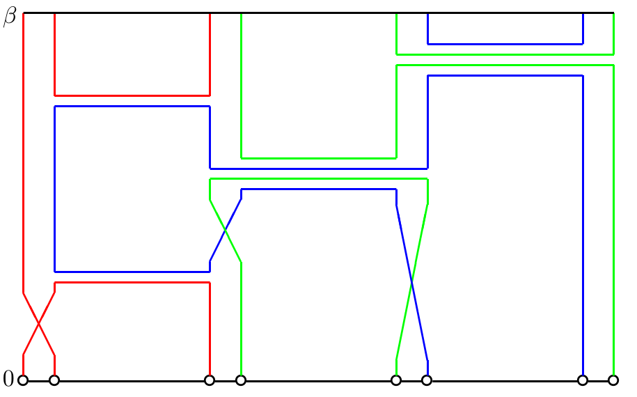
Refer to caption
Figure 3: A example realisation with loops coloured differently, here there are four sites in the underlying Λ\Lambda and for this realisation |ℒ⁡(ω)|=3|\mathcal{L}(\omega)|=3.

Note that the loops could be defined via a Poisson point process on ℰ~×[0,β]\tilde{\mathcal{E}}\times[0,\beta] where bars can occur between xix_{i} and yjy_{j} with each (i,j)(i,j) being equally likely. However one would still need to introduce the crossing or parallel events so that it is still possible to have x0x_{0} and x1x_{1} in the same loop even when there is no bar occurring on any edge containing xx.

For this loop model we have partition function

YθJ1,J2​(β,Λ)=∫ρJ1,J2​(𝑑ω)​θ|ℒ⁡(ω)|.Y_{\theta}^{J_{1},J_{2}}(\beta,\Lambda)=\int\rho_{J_{1},J_{2}}(\mathrm{d}\omega)\theta^{|\mathcal{L}(\omega)|}. (2.3)

Here θ>0\theta>0 is a parameter and ρJ1,J2\rho_{J_{1},J_{2}} is the probability measure corresponding to a Poisson point process of intensity −2​J1-2J_{1} for single bars and J2J_{2} for double bars. The relevant probability measure is then

1YθJ1,J2​(β,Λ)​ρJ1,J2​(d​ω)​θ|ℒ⁡(ω)|.\frac{1}{Y_{\theta}^{J_{1},J_{2}}(\beta,\Lambda)}\rho_{J_{1},J_{2}}(\mathrm{d}\omega)\theta^{|\mathcal{L}(\omega)|}. (2.4)

We are interested in sets of realisations, ω\omega, where certain points of Λ~×[0,β]\tilde{\Lambda}\times[0,\beta] are in the same loop. Probabilities of these events are connected to correlations in the spin-1 quantum system presented in Section 4, they will be required in the proof of Néel order in Section 6. Particular events of interest will be denoted pictorially , see Fig. 4. These events are defined and denoted as follows.

a)

The event that sites xix_{i} and yjy_{j} are connected (in the same loop). Note that the probability of xix_{i} and yjy_{j} being connected is independent of ii and jj. Denoted E[   xi      yj   ]E[\begin{picture}(0.0,0.0)\put(0.0,0.0){$\scriptsize{x_{i}}$}\put(0.9,0.15){\line{1}{0}{1.0}}\put(2.05,0.0){$\scriptsize{y_{j}}$}\end{picture}\qquad\;\,].

b)

The event that x0x_{0} and x1x_{1} are connected, y0y_{0} and y1y_{1} are connected but there is no connection from any xix_{i} to any yjy_{j}. Denoted E[   x0   x1   y0   y1                     ]E\bigg[\begin{picture}(4.7,-0.2)\put(4.75,0.75){$\scriptscriptstyle{x_{0}}$}\put(4.75,-0.75){$\scriptscriptstyle{x_{1}}$}\put(6.5,0.75){$\scriptscriptstyle{y_{0}}$}\put(6.5,-0.75){$\scriptscriptstyle{y_{1}}$}\put(5.0,-0.4){\line{0}{1}{1.0}}\put(6.75,-0.4){\line{0}{1}{1.0}}\put(5.25,0.1){\line{1}{0}{0.525}}\put(5.975,0.1){\line{1}{0}{0.525}}\put(5.775,-0.2){\line{0}{1}{0.6}}\put(5.975,-0.2){\line{0}{1}{0.6}}\end{picture}\qquad\bigg].

c)

The event that x0x_{0} and y0y_{0} are connected, x1x_{1} and y1y_{1} are connected but x0x_{0} and x1x_{1} are not connected. Denoted E[   x0   x1   y0   y1                     ]E\bigg[\begin{picture}(8.8,-0.2)\put(8.75,0.75){$\scriptscriptstyle{x_{0}}$}\put(8.75,-0.75){$\scriptscriptstyle{x_{1}}$}\put(10.5,0.75){$\scriptscriptstyle{y_{0}}$}\put(10.5,-0.75){$\scriptscriptstyle{y_{1}}$}\put(9.5,0.875){\line{1}{0}{1.0}}\put(9.5,-0.625){\line{1}{0}{1.0}}\put(10.0,-0.5){\line{0}{1}{0.5}}\put(9.7,0.0){\line{1}{0}{0.6}}\put(9.7,0.2){\line{1}{0}{0.6}}\put(10.0,0.2){\line{0}{1}{0.5}}\end{picture}\qquad\bigg]. We can also have x0x_{0} and y1y_{1} connected and x1x_{1} and y0y_{0} connected but x0x_{0} and x1x_{1} not connected and denote the event in the analogous way. These events both have the same probability.

d)

The event that all four sites x0,x1,y0,y1x_{0},x_{1},y_{0},y_{1} are connected. Denoted E[   x0   x1   y0   y1                     ]E\bigg[\begin{picture}(12.8,-0.2)\put(12.75,0.75){$\scriptscriptstyle{x_{0}}$}\put(12.75,-0.75){$\scriptscriptstyle{x_{1}}$}\put(14.5,0.75){$\scriptscriptstyle{y_{0}}$}\put(14.5,-0.75){$\scriptscriptstyle{y_{1}}$}\put(13.4,0.875){\line{1}{0}{1.0}}\put(14.4,-0.625){\line{-1}{0}{1.0}}\put(13.25,-0.525){\line{1}{1}{1.2}}\put(14.55,-0.425){\line{-1}{1}{1.2}}\put(13.0,-0.4){\line{0}{1}{1.0}}\put(14.75,0.6){\line{0}{-1}{1.0}}\end{picture}\qquad\bigg].

The definition of bars means that if a loop is followed starting from a point xi∈Λ~x_{i}\in\tilde{\Lambda} (by moving in either the up or down direction) then the direction it is travelling upon arriving at a point yj∈Λ~y_{j}\in\tilde{\Lambda} in the same loop is determined only by the number of bars the loop has encountered between the sites. For example on a bipartite lattice defined by sublattices ΛA\Lambda_{A} and ΛB\Lambda_{B} such that {x,y}∈ℰ⇔x∈ΛA,y∈ΛB\{x,y\}\in\mathcal{E}\iff x\in\Lambda_{A},y\in\Lambda_{B} the direction that xix_{i} is left and yjy_{j} is entered will be the same if xx and yy are in the same sublattice and different if they are in different sublattices.

Sometimes the order in which sites are encountered along the loop will be important. In this case arrows will indicate the order that sites will be encountered in on following the loop (up to parameterisation). The events E[   x0   x1   y0   y1               ]E\bigg[\begin{picture}(12.8,-0.2)\put(12.75,0.75){$\scriptscriptstyle{x_{0}}$}\put(12.75,-0.75){$\scriptscriptstyle{x_{1}}$}\put(14.5,0.75){$\scriptscriptstyle{y_{0}}$}\put(14.5,-0.75){$\scriptscriptstyle{y_{1}}$}\put(13.5,0.875){\vector{1}{0}{1.0}}\put(14.4,-0.625){\vector{-1}{0}{1.0}}\put(13.0,-0.4){\vector{0}{1}{1.0}}\put(14.75,0.6){\vector{0}{-1}{1.0}}\end{picture}\qquad\bigg] , E[   x0   x1   y0   y1               ]E\bigg[\begin{picture}(12.8,-0.2)\put(12.75,0.75){$\scriptscriptstyle{x_{0}}$}\put(12.75,-0.75){$\scriptscriptstyle{x_{1}}$}\put(14.5,0.75){$\scriptscriptstyle{y_{0}}$}\put(14.5,-0.75){$\scriptscriptstyle{y_{1}}$}\put(13.25,-0.525){\vector{1}{1}{1.2}}\put(14.55,-0.525){\vector{-1}{1}{1.2}}\put(13.0,0.6){\vector{0}{-1}{1.0}}\put(14.75,0.6){\vector{0}{-1}{1.0}}\end{picture}\qquad\bigg]  and E[   x0   x1   y0   y1               ]E\bigg[\begin{picture}(12.8,-0.2)\put(12.75,0.75){$\scriptscriptstyle{x_{0}}$}\put(12.75,-0.75){$\scriptscriptstyle{x_{1}}$}\put(14.5,0.75){$\scriptscriptstyle{y_{0}}$}\put(14.5,-0.75){$\scriptscriptstyle{y_{1}}$}\put(14.4,0.875){\vector{-1}{0}{1.0}}\put(14.4,-0.625){\vector{-1}{0}{1.0}}\put(13.25,-0.525){\vector{1}{1}{1.2}}\put(13.25,0.575){\vector{1}{-1}{1.2}}\end{picture}\qquad\bigg]  are the events that all four sites are connected and are encountered along the loop in the order indicated by the arrows. For example the first event,E[   x0   x1   y0   y1               ]E\bigg[\begin{picture}(12.8,-0.2)\put(12.75,0.75){$\scriptscriptstyle{x_{0}}$}\put(12.75,-0.75){$\scriptscriptstyle{x_{1}}$}\put(14.5,0.75){$\scriptscriptstyle{y_{0}}$}\put(14.5,-0.75){$\scriptscriptstyle{y_{1}}$}\put(13.5,0.875){\vector{1}{0}{1.0}}\put(14.4,-0.625){\vector{-1}{0}{1.0}}\put(13.0,-0.4){\vector{0}{1}{1.0}}\put(14.75,0.6){\vector{0}{-1}{1.0}}\end{picture}\qquad\bigg], means that upon leaving site x0x_{0} if we encounter y0y_{0} before encountering x1x_{1} then we will then encounter y1y_{1} and then x1x_{1} before closing the loop. As this notation is potentially confusing (but also seemingly unavoidable) the reader will be told explicitly when the order is important. When wanting the probability of these events we will drop the EE from the notation, as below.

It is intuitively clear that ℙ(   x0      y0   )\mathbb{P}(\begin{picture}(0.0,0.0)\put(0.0,0.0){$\scriptsize{x_{0}}$}\put(0.9,0.15){\line{1}{0}{1.0}}\put(2.05,0.0){$\scriptsize{y_{0}}$}\end{picture}\qquad\;\,) decays exponentially fast with respect to ‖x−y‖\|x-y\| for β\beta small. Hence ℙ(   x0   x1   y0   y1                     )\mathbb{P}\bigg(\begin{picture}(12.8,-0.2)\put(12.75,0.75){$\scriptscriptstyle{x_{0}}$}\put(12.75,-0.75){$\scriptscriptstyle{x_{1}}$}\put(14.5,0.75){$\scriptscriptstyle{y_{0}}$}\put(14.5,-0.75){$\scriptscriptstyle{y_{1}}$}\put(13.4,0.875){\line{1}{0}{1.0}}\put(14.4,-0.625){\line{-1}{0}{1.0}}\put(13.25,-0.525){\line{1}{1}{1.2}}\put(14.55,-0.425){\line{-1}{1}{1.2}}\put(13.0,-0.4){\line{0}{1}{1.0}}\put(14.75,0.6){\line{0}{-1}{1.0}}\end{picture}\qquad\bigg) and ℙ(   x0   x1   y0   y1                     )\mathbb{P}\bigg(\begin{picture}(8.8,-0.2)\put(8.75,0.75){$\scriptscriptstyle{x_{0}}$}\put(8.75,-0.75){$\scriptscriptstyle{x_{1}}$}\put(10.5,0.75){$\scriptscriptstyle{y_{0}}$}\put(10.5,-0.75){$\scriptscriptstyle{y_{1}}$}\put(9.5,0.875){\line{1}{0}{1.0}}\put(9.5,-0.625){\line{1}{0}{1.0}}\put(10.0,-0.5){\line{0}{1}{0.5}}\put(9.7,0.0){\line{1}{0}{0.6}}\put(9.7,0.2){\line{1}{0}{0.6}}\put(10.0,0.2){\line{0}{1}{0.5}}\end{picture}\qquad\bigg) must also have exponential decay. ℙ(   x0   x1   y0   y1                     )\mathbb{P}\bigg(\begin{picture}(4.7,-0.2)\put(4.75,0.75){$\scriptscriptstyle{x_{0}}$}\put(4.75,-0.75){$\scriptscriptstyle{x_{1}}$}\put(6.5,0.75){$\scriptscriptstyle{y_{0}}$}\put(6.5,-0.75){$\scriptscriptstyle{y_{1}}$}\put(5.0,-0.4){\line{0}{1}{1.0}}\put(6.75,-0.4){\line{0}{1}{1.0}}\put(5.25,0.1){\line{1}{0}{0.525}}\put(5.975,0.1){\line{1}{0}{0.525}}\put(5.775,-0.2){\line{0}{1}{0.6}}\put(5.975,-0.2){\line{0}{1}{0.6}}\end{picture}\qquad\bigg) should depend weakly on ‖x−y‖\|x-y\| for small enough β\beta. For ‖x−y‖\|x-y\| large enough the probability may approach ℙ(   x0      x1   )2\mathbb{P}(\begin{picture}(0.0,0.0)\put(0.0,0.0){$\scriptsize{x_{0}}$}\put(0.9,0.15){\line{1}{0}{1.0}}\put(2.05,0.0){$\scriptsize{x_{1}}$}\end{picture}\qquad\;\;)^{2}, it is not clear how to prove or disprove such a relation at this time.

Refer to caption
Figure 4: Pictures representing the set of realisations where the pictured connections are present.

3 Space-time spin configurations

In order to make the connection with spin systems we need the notion of a space-time spin configuration. The spin system we shall connect to is the spin-1 Heisenberg model, we shall make this connection via an intertwining that merges two spin-12\frac{1}{2} models. For this reason we will take θ=2\theta=2 from Section 2 (2​S+12S+1 for S=12S=\frac{1}{2}). This is also the reason the lattice Λ~\tilde{\Lambda} has two sites for every site in Λ\Lambda. It is also possible to represent the spin-SS model for general SS by merging 2​S2S spin-12\frac{1}{2} models, this will mean Λ~\tilde{\Lambda} will have 2​S2S sites for every site in Λ\Lambda. See [18] for more details. This generalisation together with some results analogous to the ones presented here should be straightforward once the spin-1 model is understood. It is not immediately clear which results will still hold however, investigation is required.

From now on we take the cubic lattice in ℤd\mathbb{Z}^{d} with side length L, denoted ΛL\Lambda_{L}, with periodic boundary conditions. The edge set, ℰL\mathcal{E}_{L}, will consist of pairs of nearest neighbour lattice points. Precisely

ΛL=\displaystyle\Lambda_{L}= {−L2+1,…,L2}d,\displaystyle\left\{-\frac{L}{2}+1,\dots,\frac{L}{2}\right\}^{d}, (3.1)
ℰL=\displaystyle\mathcal{E}_{L}= {{x,y}⊂ΛL|∥x−y∥=1 or |xi−yi|=L−1 for some i=1,…,d}.\displaystyle\{\{x,y\}\subset\Lambda_{L}|\;\|x-y\|=1\ \text{ or }|x_{i}-y_{i}|=L-1\text{ for some }i=1,...,d\}. (3.2)

Where ‖x−y‖\|x-y\| is the graph distance between xx and yy. A space-time spin configuration is a function

σ:Λ~×[0,β]p​e​r→{−12,12}.\sigma:\tilde{\Lambda}\times[0,\beta]_{per}\to\left\{-\frac{1}{2},\frac{1}{2}\right\}. (3.3)

σxi,t\sigma_{x_{i},t} is piecewise constant in tt for any xix_{i}. We further define Σ\Sigma to be the set of all such functions with a finite number of discontinuities. For a realisation of the process ω\omega we consider σ\sigma that are constant on the vertical segments of each loop in ℒ⁡(ω)\mathcal{L}(\omega) and that change value on crossing a bar. This restriction on configurations will allow to make the link with spin systems. We call such configurations compatible with ω\omega and denote by Σ(1)​(ω)\Sigma^{(1)}(\omega) the set of all compatible configurations. The following relation holds as we work on a bipartite lattice, meaning fixing a configuration’s value at some (xi,t)(x_{i},t) determines the configuration on the entire loop containing (xi,t)(x_{i},t):

|Σ(1)​(ω)|=2|ℒ⁡(ω)|,|\Sigma^{(1)}(\omega)|=2^{|\mathcal{L}(\omega)|}, (3.4)

from which we can obtain

Y2J1,J2​(β,Λ)=∫ρJ1,J2​(𝑑ω)​∑σ∈Σ(1)​(ω)1.Y_{2}^{J_{1},J_{2}}(\beta,\Lambda)=\int\rho_{J_{1},J_{2}}(\mathrm{d}\omega)\sum_{\sigma\in\Sigma^{(1)}(\omega)}1. (3.5)

We further define the set Σxi,yj(1)​(ω)⊃Σ(1)​(ω)\Sigma^{(1)}_{x_{i},y_{j}}(\omega)\supset\Sigma^{(1)}(\omega) to be compatible configurations along with configurations that flip spin at points (xi,0)(x_{i},0) or (yj,0)(y_{j},0) (or both) but are otherwise compatible.

In the remainder of this section it will be convenient to ignore the condition that compatible configurations flip value on crossing a bars as it adds unnecessary extra complication. Hence we further define Σ(2)​(ω)\Sigma^{(2)}(\omega) to be configurations that are constant on loops (and hence do not flip value at bars). Σxi,yj(2)​(ω)⊃Σ(2)​(ω)\Sigma^{(2)}_{x_{i},y_{j}}(\omega)\supset\Sigma^{(2)}(\omega) denotes the set of configurations in Σ(2)​(ω)\Sigma^{(2)}(\omega) along with configurations that flip spin at points (xi,0)(x_{i},0) or (yj,0)(y_{j},0) (or both) but are otherwise consistent with the definition of Σ(2)​(ω)\Sigma^{(2)}(\omega). The reader should bear in mind in the sequel that the connection with the spin-1 quantum system requires spin flips at bars, with this in mind the modifications to the remainder of this section required to incorporate the spin flips are easy.

As in [23] we will later need a more general setting for the measure on space-time spin configurations. We consider a Poisson point process on ℰ~×[0,β]\tilde{\mathcal{E}}\times[0,\beta] with events being specifications of the local spin configuration. We will consider discontinuities involving two pairs of sites (x0,x1,y0,y1x_{0},x_{1},y_{0},y_{1}). The objects of the process will be a set of allowed configurations at these sites immediately before and after tt. We can denote these events as

               (3.6)
σ x 0 , t + σ x 1 , t + σ y 0 , t + σ y 1 , t + σ x 0 , t - σ x 1 , t - σ y 0 , t - σ y 1 , t -

Implicit here is an ordering on Λ\Lambda with x<yx<y. An event AA is a subset of {−1/2,1/2}8\{-1/2,1/2\}^{8} and occurs with intensity ι⁡(A)\iota(A). More precisely we let ι:𝒫({−1/2,1/2}8)→ℝ\iota:\mathcal{P}(\{-1/2,1/2\}^{8})\to\mathbb{R} denote the intensities of the Poisson point process, denoted ρι\rho_{\iota}. Given realisation, ξ\xi, of ρι\rho_{\iota} let Σ⁡(ξ)\Sigma(\xi) be the set of configurations compatible with ξ\xi meaning that σ∈Σ⁡(ξ)\sigma\in\Sigma(\xi) if

σ x 0 , t + σ x 1 , t + σ y 0 , t + σ y 1 , t + σ x 0 , t - σ x 1 , t - σ y 0 , t - σ y 1 , t -
∈A​ whenever ​ξ​ contains the event ​A​ at point ​(x0,x1,y0,y1,t),\hskip 71.13188pt\in A\text{ whenever }\xi\text{ contains the event }A\text{ at point }(x_{0},x_{1},y_{0},y_{1},t),

and σxi,t\sigma_{x_{i},t} is otherwise constant in tt. The measure is then given by ρι\rho_{\iota} with the counting measure on compatible configurations. We note that different intensities can give the same measure as in [23], for ι\iota and ι′\iota^{\prime} intensities it is shown in [23] that

∫ρι​(𝑑ξ)​∫ρι′​(d​ξ′)​∑σ∈Σ⁡(ξ∪ξ′)F⁡(σ)=∫ρι+ι′​(𝑑ξ)​∑σ∈Σ⁡(ξ)F⁡(σ).\int\rho_{\iota}(\mathrm{d}\xi)\int\rho_{\iota^{\prime}}(\mathrm{d}\xi^{\prime})\sum_{\sigma\in\Sigma(\xi\cup\xi^{\prime})}F(\sigma)=\int\rho_{\iota+\iota^{\prime}}(\mathrm{d}\xi)\sum_{\sigma\in\Sigma(\xi)}F(\sigma). (3.7)

We want to write the Poisson point process involving bars in terms of intensities of specifications of spins. We require that specifications corresponding to single and double sets of bars have intensity −2​J1-2J_{1} and J2J_{2} respectively. If we naively define ι~\tilde{\iota} by

a ′ a a b a ′ c c b a ′ a a a ′ c ′ c c c ′
ι~​({})=−2​J1,ι~​({})=J2.\tilde{\iota}\,\Bigg(\Bigg\{\qquad\qquad\quad\Bigg\}\Bigg)=-2J_{1},\qquad\tilde{\iota}\,\Bigg(\Bigg\{\qquad\qquad\quad\Bigg\}\Bigg)=J_{2}. (3.8)

For any a,a′,b,c,c′∈{1/2,−1/2}a,a^{\prime},b,c,c^{\prime}\in\{1/2,-1/2\}, where the first event corresponds to single bars and the second event to double bars. We see there is an overlap on the specification
b a a b b c c b

so this assignment of intensities of specifications cannot be correct. Simply removing the overlapping case from one of the specifications will result in events not having the required intensities. This suggests we should instead define ι\iota by a ′ a a b a ′ c c b a ′ a a a ′ c ′ c c c ′

ι⁡({}a′≠b)=−2​J1,ι⁡({}a′≠c′)=J2,\iota\,\Bigg(\Bigg\{\qquad\qquad\quad\Bigg\}_{a^{\prime}\neq b}\Bigg)=-2J_{1},\quad\iota\,\Bigg(\Bigg\{\qquad\qquad\quad\Bigg\}_{a^{\prime}\neq c^{\prime}}\Bigg)=J_{2}, (3.9)
b a a b b c c b
ι⁡({})=J2−2​J1.\iota\,\Bigg(\Bigg\{\qquad\qquad\quad\Bigg\}\Bigg)=J_{2}-2J_{1}.

For any a,a′,b,c,c′∈{1/2,−1/2}a,a^{\prime},b,c,c^{\prime}\in\{1/2,-1/2\}. Now each specification is disjoint from the other two and single and double sets of bars have intensities −2​J1-2J_{1} and J2J_{2} respectively, as required. We also have ι⁡(A)=0\iota(A)=0 for any other specification. Then

Y2J1,J2​(β,Λ)=∫ρι​(𝑑ξ)​∑σ∈Σ⁡(ξ)1.Y_{2}^{J_{1},J_{2}}(\beta,\Lambda)=\int\rho_{\iota}(\mathrm{d}\xi)\sum_{\sigma\in\Sigma(\xi)}1. (3.10)

This representation can be used to show reflection positivity of the loop model, however in light of the famous paper of Dyson, Lieb and Simon [8] showing reflection positivity for J1<0=J2J_{1}<0=J_{2} and the recent paper [16] showing reflection positivity for J1=0<J2J_{1}=0<J_{2} we have reflection positivity for J1<0<J2J_{1}<0<J_{2} more directly, as we shall see.

4 The general spin-1 SU(2) invariant Heisenberg model

Let S∈12​ℕS\in\frac{1}{2}\mathbb{N}. A spin-SS model has local Hilbert spaces ℋx=ℂ2​S+1\mathcal{H}_{x}=\mathbb{C}^{2S+1}. Observables are Hermitian matrices built from linear combinations of tensor products of operators on ⊗x∈Λℋx\otimes_{x\in\Lambda}\mathcal{H}_{x}. Physically important observables are expressed in terms of spin matrices S1,S2S^{1},S^{2} and S3S^{3}, operators on ℂ2​S+1\mathbb{C}^{2S+1} that are the generators of a (2SS+1)-dimensional irreducible unitary representation of 𝔰​𝔲​(2)\mathfrak{su}(2). They satisfy the commutation relations

[Sα,Sβ]=i​∑γℰα​β​γ​Sγ,\left[S^{\alpha},S^{\beta}\right]=i\sum_{\gamma}\mathcal{E}_{\alpha\beta\gamma}S^{\gamma}, (4.1)

where α,β,γ∈{1,2,3}\alpha,\beta,\gamma\in\{1,2,3\} and ℰα​β​γ\mathcal{E}_{\alpha\beta\gamma} is the Levi-Civita symbol. Denote 𝐒=(S1,S2,S3)\mathbf{S}=(S^{1},S^{2},S^{3}), then 𝐒⋅𝐒=S⁡(S+1)​𝟙\mathbf{S}\cdot\mathbf{S}=S(S+1)\mathbbm{1}. The case S=12S=\frac{1}{2} gives the Pauli spin matrices. For S=1S=1 there are several choices for spin matrices, we will use the following matrices:

S1=12​(010101010),S2=12​(0−i0i0−i0i0),S3=(10000000−1).S^{1}=\frac{1}{\sqrt{2}}\left(\begin{matrix}0&1&0\\ 1&0&1\\ 0&1&0\end{matrix}\right),\quad S^{2}=\frac{1}{\sqrt{2}}\left(\begin{matrix}0&-i&0\\ i&0&-i\\ 0&i&0\end{matrix}\right),\quad S^{3}=\left(\begin{matrix}1&0&0\\ 0&0&0\\ 0&0&-1\end{matrix}\right). (4.2)

Consider a pair (Λ,ℰ)(\Lambda,\mathcal{E}) of a lattice, Λ⊂ℤd\Lambda\subset\mathbb{Z}^{d}, and a set of edges, ℰ\mathcal{E}, between points in Λ\Lambda. We will take Λ\Lambda to be a box in ℤd\mathbb{Z}^{d}, hence Λ\Lambda is bipartite. We denote by ΛA\Lambda_{A} and ΛB\Lambda_{B} the two disjoint lattices such that ΛA∪ΛB=Λ\Lambda_{A}\cup\Lambda_{B}=\Lambda and every e∈ℰe\in\mathcal{E} contains precisely one site from ΛA\Lambda_{A} and one site from ΛB\Lambda_{B}.

Then we take the operator SxiS_{x}^{i} for i=1,2,3i=1,2,3 to be shorthand for the operator Sxi⊗I​dΛ∖{x}S^{i}_{x}\otimes Id_{\Lambda\setminus\{x\}}. Recall the definition of Λ~\tilde{\Lambda} and ℰ~\tilde{\mathcal{E}} above, we shall use these below.

The most general SU(2) invariant Hamiltonian with two-body interactions for spin-1 is

HΛJ1,J2=−∑{x,y}∈ℰ(J1(𝐒x⋅𝐒y)+J2(𝐒x⋅𝐒y)2).H^{J_{1},J_{2}}_{\Lambda}=-\sum_{\{x,y\}\in\mathcal{E}}\left(J_{1}\left(\mathbf{S}_{x}\cdot\mathbf{S}_{y}\right)+J_{2}\left(\mathbf{S}_{x}\cdot\mathbf{S}_{y}\right)^{2}\right). (4.3)

We will soon drop the parameters J1,J2J_{1},J_{2} from HΛJ1,J2H^{J_{1},J_{2}}_{\Lambda} for readability. In this article we will be concerned with the region where J1≤0≤J2J_{1}\leq 0\leq J_{2}. Associated to this Hamiltonian we have the following partition function and Gibbs states for β>0\beta>0:

ZΛ,βJ1,J2=\displaystyle Z_{\Lambda,\beta}^{J_{1},J_{2}}= T​r​e−β​HΛJ1,J2,\displaystyle Tre^{-\beta H^{J_{1},J_{2}}_{\Lambda}}, (4.4)
⟨⋅⟩Λ,βJ1,J2=\displaystyle\langle\cdot\rangle_{\Lambda,\beta}^{J_{1},J_{2}}= 1ZΛ,βJ1,J2​T​r⋅e−β​HΛJ1,J2.\displaystyle\frac{1}{Z_{\Lambda,\beta}^{J_{1},J_{2}}}Tr\cdot e^{-\beta H^{J_{1},J_{2}}_{\Lambda}}. (4.5)

Again we shall drop the parameters J1,J2J_{1},J_{2} from the notation.

The following new definitions come from Nachtergaele [18]. We introduce an isometry V:ℂ3→ℂ2⊗ℂ2V:\mathbb{C}^{3}\to\mathbb{C}^{2}\otimes\mathbb{C}^{2} with the property V​D1​(g)=(D12​(g))⊗2​VVD^{1}(g)=(D^{\frac{1}{2}}(g))^{\otimes 2}V for g∈S​U​(2)g\in SU(2) and DSD^{S} the spin-SS representation of SU(2). Here the representation D1D^{1} is given by the matrices (4.2) and D12D^{\frac{1}{2}} is given by the Pauli matrices. it is clear such an isometry exists as we can define it for spin matrices and then extend by linearity (recall that the spin matrices generate the representation). From this we obtain the key relation

V​Si=(σi⊗𝟙+𝟙⊗σi)​V,VS^{i}=(\sigma^{i}\otimes\mathbbm{1}+\mathbbm{1}\otimes\sigma^{i})V, (4.6)

where σi\sigma^{i} are the spin-12\frac{1}{2} matrices (hence 2​σi2\sigma^{i} are the Pauli matrices). Further we have

V∗​V=𝟙​ and ​V​V∗=P,V^{*}V=\mathbbm{1}\text{ and }VV^{*}=P, (4.7)

where PP is the projection onto the spin triplet. Hence V​SiVS^{i} acts on ℂ2⊗ℂ2\mathbb{C}^{2}\otimes\mathbb{C}^{2} and so using the notation before Vx​SxiV_{x}S_{x}^{i} acts on ⊗x∈Λℂ2⊗ℂ2\otimes_{x\in\Lambda}\mathbb{C}^{2}\otimes\mathbb{C}^{2}. We make the following definition

Ri:=V​Si​V∗.R^{i}:=VS^{i}V^{*}. (4.8)

One can check that Ri=(σi⊗𝟙+𝟙⊗σi)R^{i}=(\sigma^{i}\otimes\mathbbm{1}+\mathbbm{1}\otimes\sigma^{i}). To make expressions more concise we will also denote AX:=⊗x∈XAxA_{X}:=\otimes_{x\in X}A_{x} for X⊂ΛX\subset\Lambda. For these new operators we have a new Hamiltonian (note we have now dropped the J1J_{1} and J2J_{2} parameters)

H~Λ~(1)=−∑{x,y}∈ℰ(J1(𝐑x⋅𝐑y)+J2(𝐑x⋅𝐑y)2),\tilde{H}^{(1)}_{\tilde{\Lambda}}=-\sum_{\{x,y\}\in\mathcal{E}}\left(J_{1}\left(\mathbf{R}_{x}\cdot\mathbf{R}_{y}\right)+J_{2}\left(\mathbf{R}_{x}\cdot\mathbf{R}_{y}\right)^{2}\right), (4.9)

and associated Gibbs states

ZΛ~,β(1)=\displaystyle Z_{\tilde{\Lambda},\beta}^{(1)}= T​r​PΛ​e−β​H~Λ~(1),\displaystyle TrP_{\Lambda}e^{-\beta\tilde{H}^{(1)}_{\tilde{\Lambda}}}, (4.10)
⟨⋅⟩Λ~,β(1)=\displaystyle\langle\cdot\rangle_{\tilde{\Lambda},\beta}^{(1)}= 1ZΛ~,β∼​T​r⋅PΛ​e−β​H~Λ~(1).\displaystyle\frac{1}{Z_{\tilde{\Lambda},\beta}^{\sim}}Tr\cdot P_{\Lambda}e^{-\beta\tilde{H}^{(1)}_{\tilde{\Lambda}}}. (4.11)

The connection with the previous Gibbs state can easily be made explicit,

⟨A⟩Λ,β=⟨VΛ​A​VΛ∗⟩Λ~,β(1).\langle A\rangle_{\Lambda,\beta}=\langle V_{\Lambda}AV_{\Lambda}^{*}\rangle^{(1)}_{\tilde{\Lambda},\beta}. (4.12)

We use Dirac notation in the following way: |a,b⟩|a,b\rangle denotes an element of the one site Hilbert space ℂ2⊗ℂ2\mathbb{C}^{2}\otimes\mathbb{C}^{2} and |a,b⟩⊗|c,d⟩|a,b\rangle\otimes|c,d\rangle for two sites etc.

There are two operators of particular interest, both act on two sites. Firstly we define 𝒮(1)′\mathcal{S}^{(1)^{\prime}} by its matrix elements

⟨a′,b′|⊗⟨c′,d′|𝒮(1)′|a,b⟩⊗|c,d⟩=(−1)b−b′δa,a′δd,d′δb,−cδb′,−c′.\langle a^{\prime},b^{\prime}|\otimes\langle c^{\prime},d^{\prime}|\mathcal{S}^{(1)^{\prime}}|a,b\rangle\otimes|c,d\rangle=(-1)^{b-b^{\prime}}\delta_{a,a^{\prime}}\delta_{d,d^{\prime}}\delta_{b,-c}\delta_{b^{\prime},-c^{\prime}}. (4.13)

Geometrically this requires spin bb and cc and the spins b′b^{\prime} and c′c^{\prime} to be the negative of each other and also requires a=a′a=a^{\prime} and d=d′d=d^{\prime}. This corresponds to the the single bars in the loop picture. The second operator, 𝒟(1)′\mathcal{D}^{(1)^{\prime}}, is also defined via its matrix elements

⟨a′,b′|⊗⟨c′,d′|𝒟(1)′|a,b⟩⊗|c,d⟩=(−1)a−a′(−1)b−b′δa,−dδb,−cδa′,−d′δb′,−c′.\langle a^{\prime},b^{\prime}|\otimes\langle c^{\prime},d^{\prime}|\mathcal{D}^{(1)^{\prime}}|a,b\rangle\otimes|c,d\rangle=(-1)^{a-a^{\prime}}(-1)^{b-b^{\prime}}\delta_{a,-d}\delta_{b,-c}\delta_{a^{\prime},-d^{\prime}}\delta_{b^{\prime},-c^{\prime}}. (4.14)

The geometrical interpretation this time is that of the double bars. The actual operators needed are 𝒮(1)=P​𝒮(1)′​P\mathcal{S}^{(1)}=P\mathcal{S}^{(1)^{\prime}}P and 𝒟(1)=P​𝒟(1)′​P\mathcal{D}^{(1)}=P\mathcal{D}^{(1)^{\prime}}P in order to account for bars occurring between any xix_{i} and yjy_{j} with each ii and jj from {0,1}\{0,1\} being equally likely. Note here that from this definition we see that we require the spin value to change sign on crossing a bar as was mentioned in Section 3. There are also extra factors in 𝒮(1)\mathcal{S}^{(1)} and 𝒟(1)\mathcal{D}^{(1)} of ei​π​ae^{i\pi a} for the bottom half of a bar (denoted ⊓\sqcap) and e−i​π​ae^{-i\pi a} for the top half of a bar (denoted ⊔\sqcup) where a=±12a=\pm\frac{1}{2} is the spin value on the site in ΛA\Lambda_{A} associated to the bar. By direct computation of the matrix elements we can prove the relations

𝒮(1)x,y=−12𝐑x⋅𝐑y+12Px,y,\displaystyle\mathcal{S}^{(1)}_{x,y}=-\frac{1}{2}\mathbf{R}_{x}\cdot\mathbf{R}_{y}+\frac{1}{2}P_{x,y}, (4.15)
𝒟x,y(1)=(𝐑x⋅𝐑y)2−Px,y.\displaystyle\mathcal{D}^{(1)}_{x,y}=\left(\mathbf{R}_{x}\cdot\mathbf{R}_{y}\right)^{2}-P_{x,y}. (4.16)

Using these relations we can rewrite the Hamiltonian in the region J1≤0≤J2J_{1}\leq 0\leq J_{2} as

H~Λ~(1)=−∑{x,y}∈ℰ(−2J1𝒮x,y(1)+J2𝒟x,y(1)+(J1+J2)Px,y).\tilde{H}^{(1)}_{\tilde{\Lambda}}=-\sum_{\{x,y\}\in\mathcal{E}}\left(-2J_{1}\mathcal{S}^{(1)}_{x,y}+J_{2}\mathcal{D}^{(1)}_{x,y}+(J_{1}+J_{2})P_{x,y}\right). (4.17)

5 The random loop representation

We can neglect the term (J1+J2)​Px,y(J_{1}+J_{2})P_{x,y} in the Hamiltonian (4.17) and instead add (2​J1−J2)​𝟙(2J_{1}-J_{2})\mathbbm{1}, this does not change the Gibbs states. Doing this allows to use a useful lemma from [1]

exp{−∑{x,y}∈ℰ(uAx,y+νBx,y−u−ν)}=∫ρ(dω)∏∗(x,y)∈ω∗Cx,y.\exp\left\{-\sum_{\{x,y\}\in\mathcal{E}}\left(uA_{x,y}+\nu B_{x,y}-u-\nu\right)\right\}=\int\rho(\mathrm{d}\omega)\sideset{}{{}^{*}}{\prod}_{(x,y)\in\omega}C_{x,y}. (5.1)

Here ρ\rho is the measure associated to a Poisson point process on ℰ×[0,1]\mathcal{E}\times[0,1] with two events occurring with intensities uu and ν\nu respectively. The product is ordered according to the times at which the events occur. CC is either AA or BB depending on which event occurs. This is actually a slight extension of the lemma presented in [1]. From this we can obtain

exp{−∑{x,y}∈ℰ(−2J1𝒮x,y(1)+J2𝒟x,y(1)+2J1−J2)}=∫ρ(dω)∏∗(xi,yj)∈ω∗Axi,yj(1)\exp\left\{-\sum_{\{x,y\}\in\mathcal{E}}\left(-2J_{1}\mathcal{S}^{(1)}_{x,y}+J_{2}\mathcal{D}^{(1)}_{x,y}+2J_{1}-J_{2}\right)\right\}=\int\rho(\mathrm{d}\omega)\sideset{}{{}^{*}}{\prod}_{(x_{i},y_{j})\in\omega}A^{(1)}_{x_{i},y_{j}} (5.2)

here each A(1)A^{(1)} is one of 𝒮(1)\mathcal{S}^{(1)} or 𝒟(1)\mathcal{D}^{(1)}. The process has intensity −2​J1-2J_{1} for single bars and J2J_{2} for double bars. Again the product is ordered by the time events occur.

We now prove the connection between the loop model and the quantum system. This will enable us to understand certain important correlation functions. After this we should have the tools we need to calculate any two point correlation (at least ones involving only spin operators). The first thing to understand is the extra factor, which we shall denote by zxi,yj​(σ,ω)z_{x_{i},y_{j}}(\sigma,\omega), the product of all factors e±i​π​ae^{\pm i\pi a} from operators 𝒮(1)\mathcal{S}^{(1)} and 𝒟(1)\mathcal{D}^{(1)} corresponding to the bars in loop(s) containing xix_{i} and yjy_{j} in a realisation ω\omega of ρJ1,J2\rho_{J_{1},J_{2}}. Again a∈{1/2,−1/2}a\in\{1/2,-1/2\} is the value that σ\sigma assigns to the portions of these loop(s) in the ΛA\Lambda_{A} sublattice (or if all of a loop is on the sublattice ΛB\Lambda_{B} aa is given by the negative of the value assigned to the loop). The value of zxi,yj​(σ,ω)z_{x_{i},y_{j}}(\sigma,\omega) is specified by the following lemma:

Lemma 5.1.

For Λ\Lambda bipartite we have for all i,ji,j

zxi,yj​(σ,ω)={1 if ​σ∈Σ(1)​(ω)(−1)‖x−y‖ if σ∈Σ(1)xi,yj(ω)∖Σ(1)(ω) and ω∈E[   xi      yj   ].z_{x_{i},y_{j}}(\sigma,\omega)=\left\{\begin{array}[]{c l}1&\text{ if }\sigma\in\Sigma^{(1)}(\omega)\\ (-1)^{\|x-y\|}&\text{ if }\sigma\in\Sigma^{(1)}_{x_{i},y_{j}}(\omega)\setminus\Sigma^{(1)}(\omega)\text{ and }\omega\in E[\begin{picture}(0.0,0.0)\put(0.0,0.0){$\scriptsize{x_{i}}$}\put(0.9,0.15){\line{1}{0}{1.0}}\put(2.05,0.0){$\scriptsize{y_{j}}$}\end{picture}\qquad\;\,].\\ \end{array}\right. (5.3)

Before the proof we should note that the lemma says that the only dependence on σ\sigma is at xix_{i} and yjy_{j} at time zero. If the spin does not flip at both sites that we get total factor 11, else it depends on which sublattices the sites are in. If the spin only flips at one site then there are no compatible configurations hence the value of the total extra factor is unimportant.

Proof.

To begin note that we can take (i,j)=(0,0)(i,j)=(0,0). The result for (i,j)≠(0,0)(i,j)\neq(0,0) follows as the choice of ii or jj does not affect which sublattice the two sites are in. Suppose σ∈Σ(1)​(ω)\sigma\in\Sigma^{(1)}(\omega). Moving upwards from x0x_{0} the first bar encountered is ⊓\sqcap, the bars encountered then alternate between ⊔\sqcup and ⊓\sqcap. Moving downwards from x0x_{0} we first encounter a bar ⊔\sqcup then alternate between ⊓\sqcap and ⊔\sqcup. This means we can make a matching between bars of the form ⊓\sqcap and bars of the form ⊔\sqcup. Because there are no spin flips at time zero all the bars ⊓\sqcap have factors ei​π​ae^{i\pi a} and all the bars ⊔\sqcup have factor e−i​π​ae^{-i\pi a} where aa is the spin value σ\sigma gives to x0x_{0} at time zero. Hence we have full cancellation and are left with factor 11. If there were a spin flip then bars between x0x_{0} at time 0−0- and y0y_{0} at time 0±0\pm would have factors ei​π​(−a)e^{i\pi(-a)} and e−i​π​(−a)e^{-i\pi(-a)} for ⊓\sqcap and ⊔\sqcup respectively.

If σ∈Σx0,y0(1)​(ω)∖Σ(1)​(ω)\sigma\in\Sigma^{(1)}_{x_{0},y_{0}}(\omega)\setminus\Sigma^{(1)}(\omega) and (−1)‖x−y‖=1(-1)^{\|x-y\|}=1 and ω∈E[   x0      y0   ]\omega\in E[\begin{picture}(0.0,0.0)\put(0.0,0.0){$\scriptsize{x_{0}}$}\put(0.9,0.15){\line{1}{0}{1.0}}\put(2.05,0.0){$\scriptsize{y_{0}}$}\end{picture}\qquad\;\,], then x0x_{0} and y0y_{0} are in the same sublattice. We can thus deduce that the section of loop that moves upwards/downwards from x0x_{0} crosses an even number of bars before reaching y0y_{0}. This means that the loop containing x0x_{0} and y0y_{0} contains an even number of bars of each type (⊓\sqcap or ⊔\sqcup). Hence we can make a matching of a bar ⊔\sqcup in one ‘half’ of the loop with a bar ⊔\sqcup in the other ‘half’ and the same with bars ⊓\sqcap, with some bars left over. The factors from bars in the matching will thus be 11 as the spin flip at x0x_{0} at time 00 means one bar in each pair has factor e±i​π​ae^{\pm i\pi a} and one bar has factor e±i​π​(−a)e^{\pm i\pi(-a)}. Here by ‘half’ of a loop we mean the section that connects x0x_{0} at time 0+0+ with y0y_{0} at time 0−0- or x0x_{0} at time 0−0- with y0y_{0} at time 0+0+. There are still possibly some bars left over as each half of the loop may have a different number of bars in it. A moments thought reveals that there must be an even number of bars left, half of type ⊓\sqcap and half of type ⊔\sqcup. As the bars ⊓\sqcap have factor e−i​π​(±a)e^{-i\pi(\pm a)} and the bars ⊔\sqcup have factor ei​π​(±a)e^{i\pi(\pm a)} we have full cancellation again and have total factor 11.

For the remaining case σ∈Σx0,y0(1)​(ω)∖Σ(1)​(ω)\sigma\in\Sigma^{(1)}_{x_{0},y_{0}}(\omega)\setminus\Sigma^{(1)}(\omega) and (−1)‖x−y‖=−1(-1)^{\|x-y\|}=-1 and ω∈E[   x0      y0   ]\omega\in E[\begin{picture}(0.0,0.0)\put(0.0,0.0){$\scriptsize{x_{0}}$}\put(0.9,0.15){\line{1}{0}{1.0}}\put(2.05,0.0){$\scriptsize{y_{0}}$}\end{picture}\qquad\;\,], we have x0x_{0} and y0y_{0} in different sublattices. We can see as last time that the factors from the ‘extra bars’ (that arise from each half of the loop having a different number of bars) will cancel as again there are equal numbers of ⊓\sqcap and ⊔\sqcup. For the remaining bars there are an odd number in each half of the loop, this means we can make a matching for all but two of the bars. The factors from bars in the matching will cancel each other. For the remaining two bars one is a ⊓\sqcap with factor ei​π​(±a)e^{i\pi(\pm a)} and one is a ⊔\sqcup with factor e−i​π​(∓a)e^{-i\pi(\mp a)} (the sign of aa is opposite due to the spin flip at x0x_{0} at time 00). This means the overall factor is (±i)2=−1(\pm i)^{2}=-1. This completes the proof. ∎

In light of Proposition 5.1 the following proposition can be proved in the same way as Theorem 3.2 in [23].

Proposition 5.2.

The partition functions ZΛ~,β(1)Z_{\tilde{\Lambda},\beta}^{(1)} are given by

ZΛ~,β(1)=∫ρ⁡(𝑑ω)​∑Σ(1)​(ω)∏{xi,yj}∈ℰzxi,yj​(σ,ω)=∫ρ⁡(𝑑ω)​2|ℒ⁡(ω)|=Y2J1,J2​(β,Λ).Z_{\tilde{\Lambda},\beta}^{(1)}=\int\rho(\mathrm{d}\omega)\sum_{\Sigma^{(1)}(\omega)}\prod_{\{x_{i},y_{j}\}\in\mathcal{E}}z_{x_{i},y_{j}}(\sigma,\omega)=\int\rho(\mathrm{d}\omega)2^{|\mathcal{L}(\omega)|}=Y_{2}^{J_{1},J_{2}}(\beta,\Lambda). (5.4)

We also have the following identity

T​r​(σ3⊗𝟙)x​(σ3⊗𝟙)y​e−β​H~Λ~(1)=∫ρ⁡(𝑑ω)​∑Σ(1)​(ω)(∏{xi,yj}∈ℰzxi,yj​(σ,ω))​σx0​σy0,Tr(\sigma^{3}\otimes\mathbbm{1})_{x}(\sigma^{3}\otimes\mathbbm{1})_{y}e^{-\beta\tilde{H}^{(1)}_{\tilde{\Lambda}}}=\int\rho(\mathrm{d}\omega)\sum_{\Sigma^{(1)}(\omega)}\left(\prod_{\{x_{i},y_{j}\}\in\mathcal{E}}z_{x_{i},y_{j}}(\sigma,\omega)\right)\sigma_{x_{0}}\sigma_{y_{0}}, (5.5)

where σzi\sigma_{z_{i}} is the value of a space time configuration, σ\sigma, at time 00 and site ziz_{i}.

With the important details understood we can calculate some correlations in terms of probabilities in the loop model. The most important correlations here are the Néel and nematic correlations (Proposition 5.3 (a) and (b) respectively).

Proposition 5.3.

For i,j=1,2,3i,j=1,2,3, x≠yx\neq y, i≠ji\neq j and Λ\Lambda bipartite

(a)

⟨SxiSyi⟩Λ,β=(−1)‖x−y‖ℙ(   x0      y0   )\langle S_{x}^{i}S_{y}^{i}\rangle_{\Lambda,\beta}=(-1)^{\|x-y\|}\mathbb{P}(\begin{picture}(0.0,0.0)\put(0.0,0.0){$\scriptsize{x_{0}}$}\put(0.9,0.15){\line{1}{0}{1.0}}\put(2.05,0.0){$\scriptsize{y_{0}}$}\end{picture}\qquad\;\,),

(b)

⟨(Sxi)2(Syi)2⟩Λ,β−⟨(Sxi)2⟩Λ,β⟨(Syi)2⟩Λ,β=−136+14ℙ(   x0   x1   y0   y1                     )+12ℙ(   x0   x1   y0   y1                     )+14ℙ(   x0   x1   y0   y1                     )\langle(S_{x}^{i})^{2}(S_{y}^{i})^{2}\rangle_{\Lambda,\beta}-\langle(S_{x}^{i})^{2}\rangle_{\Lambda,\beta}\langle(S_{y}^{i})^{2}\rangle_{\Lambda,\beta}=-\frac{1}{36}+\frac{1}{4}\mathbb{P}\bigg(\begin{picture}(4.7,-0.2)\put(4.75,0.75){$\scriptscriptstyle{x_{0}}$}\put(4.75,-0.75){$\scriptscriptstyle{x_{1}}$}\put(6.5,0.75){$\scriptscriptstyle{y_{0}}$}\put(6.5,-0.75){$\scriptscriptstyle{y_{1}}$}\put(5.0,-0.4){\line{0}{1}{1.0}}\put(6.75,-0.4){\line{0}{1}{1.0}}\put(5.25,0.1){\line{1}{0}{0.525}}\put(5.975,0.1){\line{1}{0}{0.525}}\put(5.775,-0.2){\line{0}{1}{0.6}}\put(5.975,-0.2){\line{0}{1}{0.6}}\end{picture}\qquad\bigg)+\frac{1}{2}\mathbb{P}\bigg(\begin{picture}(8.8,-0.2)\put(8.75,0.75){$\scriptscriptstyle{x_{0}}$}\put(8.75,-0.75){$\scriptscriptstyle{x_{1}}$}\put(10.5,0.75){$\scriptscriptstyle{y_{0}}$}\put(10.5,-0.75){$\scriptscriptstyle{y_{1}}$}\put(9.5,0.875){\line{1}{0}{1.0}}\put(9.5,-0.625){\line{1}{0}{1.0}}\put(10.0,-0.5){\line{0}{1}{0.5}}\put(9.7,0.0){\line{1}{0}{0.6}}\put(9.7,0.2){\line{1}{0}{0.6}}\put(10.0,0.2){\line{0}{1}{0.5}}\end{picture}\qquad\bigg)+\frac{1}{4}\mathbb{P}\bigg(\begin{picture}(12.8,-0.2)\put(12.75,0.75){$\scriptscriptstyle{x_{0}}$}\put(12.75,-0.75){$\scriptscriptstyle{x_{1}}$}\put(14.5,0.75){$\scriptscriptstyle{y_{0}}$}\put(14.5,-0.75){$\scriptscriptstyle{y_{1}}$}\put(13.4,0.875){\line{1}{0}{1.0}}\put(14.4,-0.625){\line{-1}{0}{1.0}}\put(13.25,-0.525){\line{1}{1}{1.2}}\put(14.55,-0.425){\line{-1}{1}{1.2}}\put(13.0,-0.4){\line{0}{1}{1.0}}\put(14.75,0.6){\line{0}{-1}{1.0}}\end{picture}\qquad\bigg),

(c)

⟨SxiSxjSyiSyj⟩Λ,β=14[−(−1)‖x−y‖ℙ(   x0      y0   )+ℙ(   x0   x1   y0   y1                     )]\langle S_{x}^{i}S_{x}^{j}S_{y}^{i}S_{y}^{j}\rangle_{\Lambda,\beta}=\frac{1}{4}\left[-(-1)^{\|x-y\|}\mathbb{P}(\begin{picture}(0.0,0.0)\put(0.0,0.0){$\scriptsize{x_{0}}$}\put(0.9,0.15){\line{1}{0}{1.0}}\put(2.05,0.0){$\scriptsize{y_{0}}$}\end{picture}\qquad\;\,)+\mathbb{P}\bigg(\begin{picture}(8.8,-0.2)\put(8.75,0.75){$\scriptscriptstyle{x_{0}}$}\put(8.75,-0.75){$\scriptscriptstyle{x_{1}}$}\put(10.5,0.75){$\scriptscriptstyle{y_{0}}$}\put(10.5,-0.75){$\scriptscriptstyle{y_{1}}$}\put(9.5,0.875){\line{1}{0}{1.0}}\put(9.5,-0.625){\line{1}{0}{1.0}}\put(10.0,-0.5){\line{0}{1}{0.5}}\put(9.7,0.0){\line{1}{0}{0.6}}\put(9.7,0.2){\line{1}{0}{0.6}}\put(10.0,0.2){\line{0}{1}{0.5}}\end{picture}\qquad\bigg)\right],

(d)

⟨SxiSxjSyjSyi⟩Λ,β=14[(−1)‖x−y‖ℙ(   x0      y0   )+ℙ(   x0   x1   y0   y1                     )]\langle S_{x}^{i}S_{x}^{j}S_{y}^{j}S_{y}^{i}\rangle_{\Lambda,\beta}=\frac{1}{4}\left[(-1)^{\|x-y\|}\mathbb{P}(\begin{picture}(0.0,0.0)\put(0.0,0.0){$\scriptsize{x_{0}}$}\put(0.9,0.15){\line{1}{0}{1.0}}\put(2.05,0.0){$\scriptsize{y_{0}}$}\end{picture}\qquad\;\,)+\mathbb{P}\bigg(\begin{picture}(8.8,-0.2)\put(8.75,0.75){$\scriptscriptstyle{x_{0}}$}\put(8.75,-0.75){$\scriptscriptstyle{x_{1}}$}\put(10.5,0.75){$\scriptscriptstyle{y_{0}}$}\put(10.5,-0.75){$\scriptscriptstyle{y_{1}}$}\put(9.5,0.875){\line{1}{0}{1.0}}\put(9.5,-0.625){\line{1}{0}{1.0}}\put(10.0,-0.5){\line{0}{1}{0.5}}\put(9.7,0.0){\line{1}{0}{0.6}}\put(9.7,0.2){\line{1}{0}{0.6}}\put(10.0,0.2){\line{0}{1}{0.5}}\end{picture}\qquad\bigg)\right],

(e)

⟨(Sxi)2(Syj)2⟩Λ,β=512+14[ℙ(   x0   x1   y0   y1                     )+ℙ(   x0   x1   y0   y1               )−ℙ(   x0   x1   y0   y1               )]\langle(S_{x}^{i})^{2}(S_{y}^{j})^{2}\rangle_{\Lambda,\beta}=\frac{5}{12}+\frac{1}{4}\left[\mathbb{P}\bigg(\begin{picture}(4.7,-0.2)\put(4.75,0.75){$\scriptscriptstyle{x_{0}}$}\put(4.75,-0.75){$\scriptscriptstyle{x_{1}}$}\put(6.5,0.75){$\scriptscriptstyle{y_{0}}$}\put(6.5,-0.75){$\scriptscriptstyle{y_{1}}$}\put(5.0,-0.4){\line{0}{1}{1.0}}\put(6.75,-0.4){\line{0}{1}{1.0}}\put(5.25,0.1){\line{1}{0}{0.525}}\put(5.975,0.1){\line{1}{0}{0.525}}\put(5.775,-0.2){\line{0}{1}{0.6}}\put(5.975,-0.2){\line{0}{1}{0.6}}\end{picture}\qquad\bigg)+\mathbb{P}\bigg(\begin{picture}(12.8,-0.2)\put(12.75,0.75){$\scriptscriptstyle{x_{0}}$}\put(12.75,-0.75){$\scriptscriptstyle{x_{1}}$}\put(14.5,0.75){$\scriptscriptstyle{y_{0}}$}\put(14.5,-0.75){$\scriptscriptstyle{y_{1}}$}\put(13.5,0.875){\vector{1}{0}{1.0}}\put(14.4,-0.625){\vector{-1}{0}{1.0}}\put(13.0,-0.4){\vector{0}{1}{1.0}}\put(14.75,0.6){\vector{0}{-1}{1.0}}\end{picture}\qquad\bigg)-\mathbb{P}\bigg(\begin{picture}(12.8,-0.2)\put(12.75,0.75){$\scriptscriptstyle{x_{0}}$}\put(12.75,-0.75){$\scriptscriptstyle{x_{1}}$}\put(14.5,0.75){$\scriptscriptstyle{y_{0}}$}\put(14.5,-0.75){$\scriptscriptstyle{y_{1}}$}\put(14.4,0.875){\vector{-1}{0}{1.0}}\put(14.4,-0.625){\vector{-1}{0}{1.0}}\put(13.25,-0.525){\vector{1}{1}{1.2}}\put(13.25,0.575){\vector{1}{-1}{1.2}}\end{picture}\qquad\bigg)\right].

Proof.

We will calculate the correlations in order. First note that each SiS^{i} plays an equivalent role, hence cyclic permutations of the indices (1,2,3)(1,2,3) does not alter the expectation. Using this together with (Si​Sj)T=±(Sj​Si)(S^{i}S^{j})^{T}=\pm(S^{j}S^{i}) (the sign depending on the value of ii and jj) means we can take i=3i=3 and j=1j=1. For each we will expand using (4.8) and (4.12).

Proof of (a). First

⟨Sx3​Sy3⟩Λ,β=⟨(σ3⊗𝟙⊗σ3⊗𝟙+σ3⊗𝟙⊗𝟙⊗σ3+𝟙⊗σ3⊗σ3⊗𝟙+𝟙⊗σ3⊗𝟙⊗σ3)x,y⟩Λ~,β(1).\langle S_{x}^{3}S_{y}^{3}\rangle_{\Lambda,\beta}=\langle(\sigma^{3}\otimes\mathbbm{1}\otimes\sigma^{3}\otimes\mathbbm{1}+\sigma^{3}\otimes\mathbbm{1}\otimes\mathbbm{1}\otimes\sigma^{3}+\mathbbm{1}\otimes\sigma^{3}\otimes\sigma^{3}\otimes\mathbbm{1}+\mathbbm{1}\otimes\sigma^{3}\otimes\mathbbm{1}\otimes\sigma^{3})_{x,y}\rangle^{(1)}_{\tilde{\Lambda},\beta}. (5.6)

We see that due to sites z0z_{0} and z1z_{1} being interchangeable for z∈Λz\in\Lambda each of the four terms in the sum have the same expectation. We also know from Proposition 5.2

T​r​(σ3⊗𝟙)x​(σ3⊗𝟙)y​e−β​H~Λ~=∫ρ⁡(𝑑ω)​∑Σ(1)​(ω)σx0​σy0.Tr(\sigma^{3}\otimes\mathbbm{1})_{x}(\sigma^{3}\otimes\mathbbm{1})_{y}e^{-\beta\tilde{H}_{\tilde{\Lambda}}}=\int\rho(\mathrm{d}\omega)\sum_{\Sigma^{(1)}(\omega)}\sigma_{x_{0}}\sigma_{y_{0}}. (5.7)

We note that the integral differs from zero only on the set where x0x_{0} and y0y_{0} are connected. If xx and yy are in different sublattices the product of spin configuration values is −14-\frac{1}{4}, if in the same sublattice the product is 14\frac{1}{4}. We can deduce that

⟨Sx3Sy3⟩Λ,β=(−1)‖x−y‖ℙ(   x0      y0   ).\langle S^{3}_{x}S^{3}_{y}\rangle_{\Lambda,\beta}=(-1)^{\|x-y\|}\mathbb{P}(\begin{picture}(0.0,0.0)\put(0.0,0.0){$\scriptsize{x_{0}}$}\put(0.9,0.15){\line{1}{0}{1.0}}\put(2.05,0.0){$\scriptsize{y_{0}}$}\end{picture}\qquad\;\,). (5.8)

Proof of (b). For the second correlation

(Rx3)2=(σ3⊗𝟙+𝟙⊗σ3)x2=(12​𝟙⊗𝟙+2​σ3⊗σ3)x.(R_{x}^{3})^{2}=(\sigma^{3}\otimes\mathbbm{1}+\mathbbm{1}\otimes\sigma^{3})^{2}_{x}=\left(\frac{1}{2}\mathbbm{1}\otimes\mathbbm{1}+2\sigma^{3}\otimes\sigma^{3}\right)_{x}. (5.9)

We see that expanding as before gives

⟨(Sx3)2⟩Λ,β=⟨(Rx3)2⟩Λ~,β(1)=1ZΛ~,β∼∫ρ(dω)∑σ∈Σ(1)​(ω)(12+2σx0σx1)=12+12ℙ(   x0      x1   ).\langle(S_{x}^{3})^{2}\rangle_{\Lambda,\beta}=\langle(R_{x}^{3})^{2}\rangle_{\tilde{\Lambda},\beta}^{(1)}=\frac{1}{Z_{\tilde{\Lambda},\beta}^{\sim}}\int\rho(\mathrm{d}\omega)\sum_{\sigma\in\Sigma^{(1)}(\omega)}\left(\frac{1}{2}+2\sigma_{x_{0}}\sigma_{x_{1}}\right)=\frac{1}{2}+\frac{1}{2}\mathbb{P}(\begin{picture}(0.0,0.0)\put(0.0,0.0){$\scriptsize{x_{0}}$}\put(0.9,0.15){\line{1}{0}{1.0}}\put(2.05,0.0){$\scriptsize{x_{1}}$}\end{picture}\qquad\;\;). (5.10)

From this and the fact that ⟨(Sx3)2⟩Λ,β=13​⟨𝐒x⋅𝐒x⟩Λ,β=23\langle(S_{x}^{3})^{2}\rangle_{\Lambda,\beta}=\frac{1}{3}\langle\mathbf{S}_{x}\cdot\mathbf{S}_{x}\rangle_{\Lambda,\beta}=\frac{2}{3} we can deduce that

ℙ(   x0      x1   )=13.\mathbb{P}(\begin{picture}(0.0,0.0)\put(0.0,0.0){$\scriptsize{x_{0}}$}\put(0.9,0.15){\line{1}{0}{1.0}}\put(2.05,0.0){$\scriptsize{x_{1}}$}\end{picture}\qquad\;\;)=\frac{1}{3}. (5.11)

For the first term in the correlation we again note that ⟨(Sx3)2​(Sy3)2⟩Λ,β=⟨(Rx3)2​(Ry3)2⟩Λ,β1\langle(S_{x}^{3})^{2}(S_{y}^{3})^{2}\rangle_{\Lambda,\beta}=\langle(R_{x}^{3})^{2}(R_{y}^{3})^{2}\rangle_{\Lambda,\beta}^{1}. We then calculate as before:

(Rx3)2​(Ry3)2=\displaystyle(R_{x}^{3})^{2}(R_{y}^{3})^{2}= (σ3⊗𝟙+𝟙⊗σ3)x2​(σ3⊗𝟙+𝟙⊗σ3)y2\displaystyle(\sigma^{3}\otimes\mathbbm{1}+\mathbbm{1}\otimes\sigma^{3})^{2}_{x}(\sigma^{3}\otimes\mathbbm{1}+\mathbbm{1}\otimes\sigma^{3})^{2}_{y} (5.12)
=\displaystyle= (12​𝟙⊗𝟙+2​σ3⊗σ3)x​(12​𝟙⊗𝟙+2​σ3⊗σ3)y\displaystyle\left(\frac{1}{2}\mathbbm{1}\otimes\mathbbm{1}+2\sigma^{3}\otimes\sigma^{3}\right)_{x}\left(\frac{1}{2}\mathbbm{1}\otimes\mathbbm{1}+2\sigma^{3}\otimes\sigma^{3}\right)_{y}
=\displaystyle= (14​𝟙⊗4+σ3⊗σ3⊗𝟙⊗𝟙+𝟙⊗𝟙⊗σ3⊗σ3+4​(σ3)⊗4)x,y.\displaystyle\left(\frac{1}{4}\mathbbm{1}^{\otimes 4}+\sigma^{3}\otimes\sigma^{3}\otimes\mathbbm{1}\otimes\mathbbm{1}+\mathbbm{1}\otimes\mathbbm{1}\otimes\sigma^{3}\otimes\sigma^{3}+4(\sigma^{3})^{\otimes 4}\right)_{x,y}.

Now following through the same expansion as before we have

⟨(Sx3)2​(Sy3)2⟩Λ,β=1Z​∫ρ⁡(𝑑ω)​∑σ∈Σ(1)​(ω)(14+σx0​σx1+σy0​σy1+4​σx0​σx1​σy0​σy1).\langle(S_{x}^{3})^{2}(S_{y}^{3})^{2}\rangle_{\Lambda,\beta}=\frac{1}{Z}\int\rho(\mathrm{d}\omega)\sum_{\sigma\in\Sigma^{(1)}(\omega)}\left(\frac{1}{4}+\sigma_{x_{0}}\sigma_{x_{1}}+\sigma_{y_{0}}\sigma_{y_{1}}+4\sigma_{x_{0}}\sigma_{x_{1}}\sigma_{y_{0}}\sigma_{y_{1}}\right). (5.13)

Using (5.11) and noting that the last term in the sum requires either two loops containing two of the sites x0,x1,y0,y1x_{0},x_{1},y_{0},y_{1} each or one loop containing all four sites to give a non-zero contribution to the sum overall (if one site is not connected to any other its spin value can be ±12\pm\frac{1}{2} independently of other sites, averaging the integral on this set to zero) we have

⟨(Sx3)2(Sy3)2⟩Λ,β−⟨(Sx3)2⟩Λ,β⟨(Sy3)2⟩Λ,β=−136+14ℙ(   x0   x1   y0   y1                     )+12ℙ(   x0   x1   y0   y1                     )+14ℙ(   x0   x1   y0   y1                     ).\langle(S_{x}^{3})^{2}(S_{y}^{3})^{2}\rangle_{\Lambda,\beta}-\langle(S_{x}^{3})^{2}\rangle_{\Lambda,\beta}\langle(S_{y}^{3})^{2}\rangle_{\Lambda,\beta}=-\frac{1}{36}+\frac{1}{4}\mathbb{P}\bigg(\begin{picture}(4.7,-0.2)\put(4.75,0.75){$\scriptscriptstyle{x_{0}}$}\put(4.75,-0.75){$\scriptscriptstyle{x_{1}}$}\put(6.5,0.75){$\scriptscriptstyle{y_{0}}$}\put(6.5,-0.75){$\scriptscriptstyle{y_{1}}$}\put(5.0,-0.4){\line{0}{1}{1.0}}\put(6.75,-0.4){\line{0}{1}{1.0}}\put(5.25,0.1){\line{1}{0}{0.525}}\put(5.975,0.1){\line{1}{0}{0.525}}\put(5.775,-0.2){\line{0}{1}{0.6}}\put(5.975,-0.2){\line{0}{1}{0.6}}\end{picture}\qquad\bigg)+\frac{1}{2}\mathbb{P}\bigg(\begin{picture}(8.8,-0.2)\put(8.75,0.75){$\scriptscriptstyle{x_{0}}$}\put(8.75,-0.75){$\scriptscriptstyle{x_{1}}$}\put(10.5,0.75){$\scriptscriptstyle{y_{0}}$}\put(10.5,-0.75){$\scriptscriptstyle{y_{1}}$}\put(9.5,0.875){\line{1}{0}{1.0}}\put(9.5,-0.625){\line{1}{0}{1.0}}\put(10.0,-0.5){\line{0}{1}{0.5}}\put(9.7,0.0){\line{1}{0}{0.6}}\put(9.7,0.2){\line{1}{0}{0.6}}\put(10.0,0.2){\line{0}{1}{0.5}}\end{picture}\qquad\bigg)+\frac{1}{4}\mathbb{P}\bigg(\begin{picture}(12.8,-0.2)\put(12.75,0.75){$\scriptscriptstyle{x_{0}}$}\put(12.75,-0.75){$\scriptscriptstyle{x_{1}}$}\put(14.5,0.75){$\scriptscriptstyle{y_{0}}$}\put(14.5,-0.75){$\scriptscriptstyle{y_{1}}$}\put(13.4,0.875){\line{1}{0}{1.0}}\put(14.4,-0.625){\line{-1}{0}{1.0}}\put(13.25,-0.525){\line{1}{1}{1.2}}\put(14.55,-0.425){\line{-1}{1}{1.2}}\put(13.0,-0.4){\line{0}{1}{1.0}}\put(14.75,0.6){\line{0}{-1}{1.0}}\end{picture}\qquad\bigg). (5.14)

The probability ℙ(   x0   x1   y0   y1                     )\mathbb{P}\bigg(\begin{picture}(8.8,-0.2)\put(8.75,0.75){$\scriptscriptstyle{x_{0}}$}\put(8.75,-0.75){$\scriptscriptstyle{x_{1}}$}\put(10.5,0.75){$\scriptscriptstyle{y_{0}}$}\put(10.5,-0.75){$\scriptscriptstyle{y_{1}}$}\put(9.5,0.875){\line{1}{0}{1.0}}\put(9.5,-0.625){\line{1}{0}{1.0}}\put(10.0,-0.5){\line{0}{1}{0.5}}\put(9.7,0.0){\line{1}{0}{0.6}}\put(9.7,0.2){\line{1}{0}{0.6}}\put(10.0,0.2){\line{0}{1}{0.5}}\end{picture}\qquad\bigg) comes with twice the weight because there are two ways to connect both sites at xx to different sites at yy (but only one way both sites at xx can be connected and both sites at yy can be connected).

Proof of (c). For the third correlation we use the same expansion

⟨S01​S03​Sx1​Sx3⟩Λ,β=4ZΛ~,β(1)​T​r​(σ1​σ3⊗𝟙+σ1⊗σ3)x​(σ1​σ3⊗𝟙+σ1⊗σ3)y​PΛ​e−β​H~Λ~(1).\langle S_{0}^{1}S_{0}^{3}S_{x}^{1}S_{x}^{3}\rangle_{\Lambda,\beta}=\frac{4}{Z_{\tilde{\Lambda},\beta}^{(1)}}Tr(\sigma^{1}\sigma^{3}\otimes\mathbbm{1}+\sigma^{1}\otimes\sigma^{3})_{x}(\sigma^{1}\sigma^{3}\otimes\mathbbm{1}+\sigma^{1}\otimes\sigma^{3})_{y}P_{\Lambda}e^{-\beta\tilde{H}^{(1)}_{\tilde{\Lambda}}}. (5.15)

The factor 44 has come from grouping together terms such as σ1⊗σ3\sigma^{1}\otimes\sigma^{3} and σ3⊗σ1\sigma^{3}\otimes\sigma^{1} that have the same expectation. A useful observation at this stage is that σ1​σ3=−i2​σ2\sigma^{1}\sigma^{3}=\frac{-i}{2}\sigma^{2}. Calculating further and noting that the two cross terms in the above product have the same expectation we see

⟨S01S03Sx1Sx3⟩Λ,β=4⟨−14σ2⊗𝟙⊗σ2⊗𝟙−iσ2⊗𝟙⊗σ1⊗σ3+σ1⊗σ3⊗σ1⊗σ3⟩Λ~,β(1).\langle S_{0}^{1}S_{0}^{3}S_{x}^{1}S_{x}^{3}\rangle_{\Lambda,\beta}=4\left\langle-\frac{1}{4}\sigma^{2}\otimes\mathbbm{1}\otimes\sigma^{2}\otimes\mathbbm{1}-i\sigma^{2}\otimes\mathbbm{1}\otimes\sigma^{1}\otimes\sigma^{3}+\sigma^{1}\otimes\sigma^{3}\otimes\sigma^{1}\otimes\sigma^{3}\right\rangle_{\tilde{\Lambda},\beta}^{(1)}. (5.16)

From the symmetric roles of σi\sigma^{i} for i=1,2,3i=1,2,3 and part a) we know the first term is −(−1)‖x−y‖4ℙ(   x0      y0   )-\frac{(-1)^{\|x-y\|}}{4}\mathbb{P}(\begin{picture}(0.0,0.0)\put(0.0,0.0){$\scriptsize{x_{0}}$}\put(0.9,0.15){\line{1}{0}{1.0}}\put(2.05,0.0){$\scriptsize{y_{0}}$}\end{picture}\qquad\;\,). For the second term we need ⟨σ2⊗𝟙⊗σ1⊗σ3⟩Λ~,β(1)\langle\sigma^{2}\otimes\mathbbm{1}\otimes\sigma^{1}\otimes\sigma^{3}\rangle_{\tilde{\Lambda},\beta}^{(1)}. This is the expectation of a matrix with purely imaginary entries, due to the one appearance of σ2\sigma^{2}. Now we note three pieces of information that allow us to calculate this expectation. All the matrices e−β​H~Λ~(1),PΛ,σ1,σ2e^{-\beta\tilde{H}^{(1)}_{\tilde{\Lambda}}},P_{\Lambda},\sigma^{1},\sigma^{2} and σ3\sigma^{3} are Hermitian. The matrices σi\sigma^{i} are acting on different sites in Λ~\tilde{\Lambda} and hence they commute. e−β​H~Λ~(1)e^{-\beta\tilde{H}^{(1)}_{\tilde{\Lambda}}} and PΛP_{\Lambda} commute and have real entries. This means taking the adjoint of the operator leaves the expectation unchanged. Because the operator is purely imaginary we should obtain the negative of what we started with on taking the adjoint. Hence the correlation must be zero.

For the last term we expand as in Proposition 5.2 and obtain

⟨σ1⊗σ3⊗σ1⊗σ3⟩Λ~,β(1)=1ZΛ~,β(1)​∫ρ⁡(𝑑ω)​∑σ∈Σx0,y0(1)​(ω)zx0,y0​(σ,ω)​⟨σ⋅,0+|σ1⊗σ3⊗σ1⊗σ3|σ⋅,0−⟩\langle\sigma^{1}\otimes\sigma^{3}\otimes\sigma^{1}\otimes\sigma^{3}\rangle_{\tilde{\Lambda},\beta}^{(1)}=\frac{1}{Z_{\tilde{\Lambda},\beta}^{(1)}}\int\rho(\mathrm{d}\omega)\sum_{\sigma\in\Sigma^{(1)}_{x_{0},y_{0}}(\omega)}z_{x_{0},y_{0}}(\sigma,\omega)\langle\sigma_{\cdot,0+}|\sigma^{1}\otimes\sigma^{3}\otimes\sigma^{1}\otimes\sigma^{3}|\sigma_{\cdot,0-}\rangle (5.17)

Here σ⋅,0±\sigma_{\cdot,0\pm} denotes the full spin configuration for some σ∈Σx0,y0​(ω)\sigma\in\Sigma_{x_{0},y_{0}}(\omega) at time 0±0\pm respectively. Also note that as σ1\sigma^{1} flips spins and σ3\sigma^{3} does not the set of space-time spin configurations Σx0,y0(1)​(ω)\Sigma^{(1)}_{x_{0},y_{0}}(\omega) is the correct set. We could expand the set of configurations we sum over to include configurations that flip spin at sites x1x_{1} and y1y_{1} at time zero but these would not be compatible with σ3\sigma^{3} acting at time zero at those sites hence they would not contribute. Recall that a loop that contains a site that spin flips at time zero cannot contain only one such site, hence the set of configurations that contribute to the integral is E[   x0      y0   ]E[\begin{picture}(0.0,0.0)\put(0.0,0.0){$\scriptsize{x_{0}}$}\put(0.9,0.15){\line{1}{0}{1.0}}\put(2.05,0.0){$\scriptsize{y_{0}}$}\end{picture}\qquad\;\,]. Again the set of configurations where one of the sites x1x_{1} or y1y_{1} is not connected to any of the other three does not contribute to the integral. Combining these two facts we see that the only sets of configurations that contribute to the integral are those where there are two loops each containing two sites (one with x0x_{0} and y0y_{0} and the other with x1x_{1} and y1y_{1}), or one loop containing all four sites. For the case of two loops there is one factor of zx0,y0​(σ,ω)=(−1)‖x−y‖z_{x_{0},y_{0}}(\sigma,\omega)=(-1)^{\|x-y\|} from the loop containing x0x_{0} and y0y_{0} (where σ1\sigma^{1} acts). Another factor of (−1)‖x−y‖(-1)^{\|x-y\|} comes from the loop containing x1x_{1} and y1y_{1} and the condition that the spin flips on crossing a bar. Note that for the first loop there is no such factor coming from spin flips at bars because σ1​|±12⟩=+12​|∓12⟩\sigma^{1}|\pm\frac{1}{2}\rangle=+\frac{1}{2}|\mp\frac{1}{2}\rangle hence there is a factor of +12+\frac{1}{2} regardless of the spin value at the site. For the case of one loop containing all sites the order that sites occur in the loop is important; this is because both σ1\sigma^{1} and σ3\sigma^{3} are acting at sites in the loop. If, when following the loop, the site y1y_{1} appears directly before or after the site x1x_{1} then the section of loop between these sites follows the normal rule of flipping spins at bars (or if we follow the loop the other way we pass through two spin flips at time zero as well, these cancel each other out as far as the product of spins at sites x1x_{1} and y1y_{1} is concerned). This means we have a factor of (−1)‖x−y‖(-1)^{\|x-y\|} as before. If one of the sites x0x_{0} or y0y_{0} appears between sites x1x_{1} and y1y_{1} on the loop the effect of the extra spin flip changes the sign of the factor coming from the product of spins, giving a factor of −(−1)‖x−y‖-(-1)^{\|x-y\|}. As before we also have the factor zx0,y0​(σ,ω)=(−1)‖x−y‖z_{x_{0},y_{0}}(\sigma,\omega)=(-1)^{\|x-y\|} in both cases. This means the correlation is

⟨σ1⊗σ3⊗σ1⊗σ3⟩Λ~,β(1)=116[ℙ(   x0   x1   y0   y1                     )+ℙ(   x0   x1   y0   y1               )−ℙ(   x0   x1   y0   y1               )].\langle\sigma^{1}\otimes\sigma^{3}\otimes\sigma^{1}\otimes\sigma^{3}\rangle_{\tilde{\Lambda},\beta}^{(1)}=\frac{1}{16}\left[\mathbb{P}\bigg(\begin{picture}(8.8,-0.2)\put(8.75,0.75){$\scriptscriptstyle{x_{0}}$}\put(8.75,-0.75){$\scriptscriptstyle{x_{1}}$}\put(10.5,0.75){$\scriptscriptstyle{y_{0}}$}\put(10.5,-0.75){$\scriptscriptstyle{y_{1}}$}\put(9.5,0.875){\line{1}{0}{1.0}}\put(9.5,-0.625){\line{1}{0}{1.0}}\put(10.0,-0.5){\line{0}{1}{0.5}}\put(9.7,0.0){\line{1}{0}{0.6}}\put(9.7,0.2){\line{1}{0}{0.6}}\put(10.0,0.2){\line{0}{1}{0.5}}\end{picture}\qquad\bigg)+\mathbb{P}\bigg(\begin{picture}(12.8,-0.2)\put(12.75,0.75){$\scriptscriptstyle{x_{0}}$}\put(12.75,-0.75){$\scriptscriptstyle{x_{1}}$}\put(14.5,0.75){$\scriptscriptstyle{y_{0}}$}\put(14.5,-0.75){$\scriptscriptstyle{y_{1}}$}\put(13.5,0.875){\vector{1}{0}{1.0}}\put(14.4,-0.625){\vector{-1}{0}{1.0}}\put(13.0,-0.4){\vector{0}{1}{1.0}}\put(14.75,0.6){\vector{0}{-1}{1.0}}\end{picture}\qquad\bigg)-\mathbb{P}\bigg(\begin{picture}(12.8,-0.2)\put(12.75,0.75){$\scriptscriptstyle{x_{0}}$}\put(12.75,-0.75){$\scriptscriptstyle{x_{1}}$}\put(14.5,0.75){$\scriptscriptstyle{y_{0}}$}\put(14.5,-0.75){$\scriptscriptstyle{y_{1}}$}\put(13.25,-0.525){\vector{1}{1}{1.2}}\put(14.55,-0.525){\vector{-1}{1}{1.2}}\put(13.0,0.6){\vector{0}{-1}{1.0}}\put(14.75,0.6){\vector{0}{-1}{1.0}}\end{picture}\qquad\bigg)\right]. (5.18)

Recall that the arrows in the events show the direction that the loop is traversed. From this we can finally deduce that

⟨Sx1Sx3Sy1Sy3⟩Λ,β=14[−(−1)‖x−y‖ℙ(   x0      y0   )+ℙ(   x0   x1   y0   y1                     )+ℙ(   x0   x1   y0   y1               )−ℙ(   x0   x1   y0   y1               )].\langle S_{x}^{1}S_{x}^{3}S_{y}^{1}S_{y}^{3}\rangle_{\Lambda,\beta}=\frac{1}{4}\left[-(-1)^{\|x-y\|}\mathbb{P}(\begin{picture}(0.0,0.0)\put(0.0,0.0){$\scriptsize{x_{0}}$}\put(0.9,0.15){\line{1}{0}{1.0}}\put(2.05,0.0){$\scriptsize{y_{0}}$}\end{picture}\qquad\;\,)+\mathbb{P}\bigg(\begin{picture}(8.8,-0.2)\put(8.75,0.75){$\scriptscriptstyle{x_{0}}$}\put(8.75,-0.75){$\scriptscriptstyle{x_{1}}$}\put(10.5,0.75){$\scriptscriptstyle{y_{0}}$}\put(10.5,-0.75){$\scriptscriptstyle{y_{1}}$}\put(9.5,0.875){\line{1}{0}{1.0}}\put(9.5,-0.625){\line{1}{0}{1.0}}\put(10.0,-0.5){\line{0}{1}{0.5}}\put(9.7,0.0){\line{1}{0}{0.6}}\put(9.7,0.2){\line{1}{0}{0.6}}\put(10.0,0.2){\line{0}{1}{0.5}}\end{picture}\qquad\bigg)+\mathbb{P}\bigg(\begin{picture}(12.8,-0.2)\put(12.75,0.75){$\scriptscriptstyle{x_{0}}$}\put(12.75,-0.75){$\scriptscriptstyle{x_{1}}$}\put(14.5,0.75){$\scriptscriptstyle{y_{0}}$}\put(14.5,-0.75){$\scriptscriptstyle{y_{1}}$}\put(13.5,0.875){\vector{1}{0}{1.0}}\put(14.4,-0.625){\vector{-1}{0}{1.0}}\put(13.0,-0.4){\vector{0}{1}{1.0}}\put(14.75,0.6){\vector{0}{-1}{1.0}}\end{picture}\qquad\bigg)-\mathbb{P}\bigg(\begin{picture}(12.8,-0.2)\put(12.75,0.75){$\scriptscriptstyle{x_{0}}$}\put(12.75,-0.75){$\scriptscriptstyle{x_{1}}$}\put(14.5,0.75){$\scriptscriptstyle{y_{0}}$}\put(14.5,-0.75){$\scriptscriptstyle{y_{1}}$}\put(13.25,-0.525){\vector{1}{1}{1.2}}\put(14.55,-0.525){\vector{-1}{1}{1.2}}\put(13.0,0.6){\vector{0}{-1}{1.0}}\put(14.75,0.6){\vector{0}{-1}{1.0}}\end{picture}\qquad\bigg)\right]. (5.19)

Now we note that the last two probabilities are equal (swap y0y_{0} and y1y_{1}).

The correlations (d) and (e) follow easily using the same techniques and considerations as above. ∎

From this we can easily obtain some bounds on these correlations that are potentially very difficult to obtain without the loop model.

Corollary 5.4.

For i,j=1,2,3i,j=1,2,3, x≠yx\neq y, i≠ji\neq j and Λ\Lambda bipartite

(a)

⟨(Sxi)2​(Syi)2⟩Λ,β−⟨(Sx3)2⟩Λ,β​⟨(Sy3)2⟩Λ,β≤118+34​(−1)‖x−y‖​⟨Sxi​Syi⟩Λ,β\langle(S_{x}^{i})^{2}(S_{y}^{i})^{2}\rangle_{\Lambda,\beta}-\langle(S_{x}^{3})^{2}\rangle_{\Lambda,\beta}\langle(S_{y}^{3})^{2}\rangle_{\Lambda,\beta}\leq\frac{1}{18}+\frac{3}{4}(-1)^{\|x-y\|}\langle S_{x}^{i}S_{y}^{i}\rangle_{\Lambda,\beta}

(b)

⟨Sxi​Sxj​Syi​Syj⟩Λ,β≤14​((−1)‖x−y‖−1)​⟨Sxi​Syi⟩Λ,β\langle S_{x}^{i}S_{x}^{j}S_{y}^{i}S_{y}^{j}\rangle_{\Lambda,\beta}\leq\frac{1}{4}((-1)^{\|x-y\|}-1)\langle S_{x}^{i}S_{y}^{i}\rangle_{\Lambda,\beta}

(c)

⟨Sxi​Sxj​Syj​Syj⟩Λ,β≤14​((−1)‖x−y‖+1)​⟨Sxi​Syi⟩Λ,β\langle S_{x}^{i}S_{x}^{j}S_{y}^{j}S_{y}^{j}\rangle_{\Lambda,\beta}\leq\frac{1}{4}((-1)^{\|x-y\|}+1)\langle S_{x}^{i}S_{y}^{i}\rangle_{\Lambda,\beta}

(d)

⟨Sxi​Sxj​Syi​Syj⟩Λ,β​{≥0if ‖x−y‖ is odd≤0if ‖x−y‖ is even\langle S_{x}^{i}S_{x}^{j}S_{y}^{i}S_{y}^{j}\rangle_{\Lambda,\beta}\left\{\begin{array}[]{l l}\geq 0&\quad\text{if $\|x-y\|$ is odd}\\ \leq 0&\quad\text{if $\|x-y\|$ is even}\end{array}\right.

(e)

⟨Sxi​Sxj​Syj​Syi⟩Λ,β​{≤0if ‖x−y‖ is odd≥0if ‖x−y‖ is even\langle S_{x}^{i}S_{x}^{j}S_{y}^{j}S_{y}^{i}\rangle_{\Lambda,\beta}\left\{\begin{array}[]{l l}\leq 0&\quad\text{if $\|x-y\|$ is odd}\\ \geq 0&\quad\text{if $\|x-y\|$ is even}\end{array}\right.

Proof.

All inequalities are immediate from Proposition 5.3 when we note that E[   x0   x1   y0   y1                     ]E\bigg[\begin{picture}(4.7,-0.2)\put(4.75,0.75){$\scriptscriptstyle{x_{0}}$}\put(4.75,-0.75){$\scriptscriptstyle{x_{1}}$}\put(6.5,0.75){$\scriptscriptstyle{y_{0}}$}\put(6.5,-0.75){$\scriptscriptstyle{y_{1}}$}\put(5.0,-0.4){\line{0}{1}{1.0}}\put(6.75,-0.4){\line{0}{1}{1.0}}\put(5.25,0.1){\line{1}{0}{0.525}}\put(5.975,0.1){\line{1}{0}{0.525}}\put(5.775,-0.2){\line{0}{1}{0.6}}\put(5.975,-0.2){\line{0}{1}{0.6}}\end{picture}\qquad\bigg] is a sub-event of E[   x0      x1   ]E[\begin{picture}(0.0,0.0)\put(0.0,0.0){$\scriptsize{x_{0}}$}\put(0.9,0.15){\line{1}{0}{1.0}}\put(2.05,0.0){$\scriptsize{x_{1}}$}\end{picture}\qquad\;\,] and E[   x0   x1   y0   y1                     ]E\bigg[\begin{picture}(8.8,-0.2)\put(8.75,0.75){$\scriptscriptstyle{x_{0}}$}\put(8.75,-0.75){$\scriptscriptstyle{x_{1}}$}\put(10.5,0.75){$\scriptscriptstyle{y_{0}}$}\put(10.5,-0.75){$\scriptscriptstyle{y_{1}}$}\put(9.5,0.875){\line{1}{0}{1.0}}\put(9.5,-0.625){\line{1}{0}{1.0}}\put(10.0,-0.5){\line{0}{1}{0.5}}\put(9.7,0.0){\line{1}{0}{0.6}}\put(9.7,0.2){\line{1}{0}{0.6}}\put(10.0,0.2){\line{0}{1}{0.5}}\end{picture}\qquad\bigg] is a sub-event of E[   x0      y0   ]E[\begin{picture}(0.0,0.0)\put(0.0,0.0){$\scriptsize{x_{0}}$}\put(0.9,0.15){\line{1}{0}{1.0}}\put(2.05,0.0){$\scriptsize{y_{0}}$}\end{picture}\qquad\;\,]. ∎

Other inequalities of interest involve correlations between nearest neighbour points. Equation (29) in [20] allows us to obtain the following bound in the ground state (β→∞\beta\to\infty)

ℙ(   00      e10   )≥1d2​J2−3​J14​J2−3​J1.\mathbb{P}(\begin{picture}(0.0,0.0)\put(0.0,0.0){$\scriptsize{0_{0}}$}\put(0.9,0.15){\line{1}{0}{1.0}}\put(2.05,0.0){$\scriptsize{e_{1_{0}}}$}\end{picture}\qquad\quad)\geq\frac{1}{d}\frac{2J_{2}-3J_{1}}{4J_{2}-3J_{1}}. (5.20)

Now looking at Proposition 5.3 (b) for ‖x−y‖=1\|x-y\|=1 (say x=0x=0, y=e1y=e_{1}) we see that if J1=0J_{1}=0 then the event ℙ(   00      e10   )\mathbb{P}(\begin{picture}(0.0,0.0)\put(0.0,0.0){$\scriptsize{0_{0}}$}\put(0.9,0.15){\line{1}{0}{1.0}}\put(2.05,0.0){$\scriptsize{e_{1_{0}}}$}\end{picture}\qquad\quad) puts us into the case of one of the last two probabilities. Ignoring the first probability (as it is difficult to control) we obtain (for J2>0=J1J_{2}>0=J_{1})

⟨(S03)2​(Se13)2⟩Λ,β−⟨(S03)2⟩Λ,β​⟨(Se13)2⟩Λ,β≥−136+18​d.\langle(S_{0}^{3})^{2}(S_{e_{1}}^{3})^{2}\rangle_{\Lambda,\beta}-\langle(S_{0}^{3})^{2}\rangle_{\Lambda,\beta}\langle(S_{e_{1}}^{3})^{2}\rangle_{\Lambda,\beta}\geq-\frac{1}{36}+\frac{1}{8d}. (5.21)

This bound is positive for d≤4d\leq 4, however it was not sufficient to deduce nematic order from a theorem analogous to 6.1 but concerning the nematic correlation function.

6 Occurrence of Néel Order

6.1 Setting and results

We take the cubic lattice in ℤd\mathbb{Z}^{d} with side length L, denoted ΛL\Lambda_{L}, with periodic boundary conditions. The edge set, ℰL\mathcal{E}_{L}, will consist of pairs of nearest neighbour lattice points. Precisely

ΛL=\displaystyle\Lambda_{L}= {−L2+1,…,L2}d,\displaystyle\left\{-\frac{L}{2}+1,\dots,\frac{L}{2}\right\}^{d}, (6.1)
ℰL=\displaystyle\mathcal{E}_{L}= {{x,y}⊂ΛL|∥x−y∥=1 or |xi−yi|=L−1 for some i=1,…,d}.\displaystyle\{\{x,y\}\subset\Lambda_{L}|\;\|x-y\|=1\ \text{ or }|x_{i}-y_{i}|=L-1\text{ for some }i=1,...,d\}. (6.2)

For the main theorem we need to introduce two integrals, they come about due to similar considerations as in [15]

Id=\displaystyle I_{d}= 1(2​π)d​∫[−π,π]d(1d​∑i=1dcos⁡ki)+​ε⁡(k+π)ε⁡(k)​𝑑k,\displaystyle\frac{1}{(2\pi)^{d}}\int_{[-\pi,\pi]^{d}}\left(\frac{1}{d}\sum_{i=1}^{d}\cos k_{i}\right)_{+}\sqrt{\frac{\varepsilon(k+\pi)}{\varepsilon(k)}}\mathrm{d}k, (6.3)
Kd=\displaystyle K_{d}= 1(2​π)d​∫[−π,π]dε⁡(k+π)ε⁡(k)​𝑑k.\displaystyle\frac{1}{(2\pi)^{d}}\int_{[-\pi,\pi]^{d}}\sqrt{\frac{\varepsilon(k+\pi)}{\varepsilon(k)}}\mathrm{d}k. (6.4)

Here (⋅)+(\cdot)_{+} denotes the positive part and ε⁡(k)=2​∑i=1d(1−cos⁡(ki))\varepsilon(k)=2\sum_{i=1}^{d}(1-\cos(k_{i})).

Theorem 6.1.

Let d≥3d\geq 3 and J1≤0≤J2J_{1}\leq 0\leq J_{2}, for LL even we have the two bounds

limβ→∞limL→∞1|ΛL|​∑x∈ΛL(−1)‖x‖​⟨S03​Sx3⟩ΛL,βJ1,J2≥{ℙ(   00      e10   )​(ℙ(   00      e10   )−Id​14−J2J1),1−Kd​ℙ(   00      e10   )​14−J2J1.\displaystyle\lim_{\beta\to\infty}\lim_{L\to\infty}\frac{1}{|\Lambda_{L}|}\sum_{x\in\Lambda_{L}}(-1)^{\|x\|}\langle S_{0}^{3}S_{x}^{3}\rangle^{J_{1},J_{2}}_{\Lambda_{L},\beta}\geq\begin{cases}\sqrt{\mathbb{P}(\begin{picture}(0.0,0.0)\put(0.0,0.0){$\scriptsize{0_{0}}$}\put(0.9,0.15){\line{1}{0}{1.0}}\put(2.05,0.0){$\scriptsize{e_{1_{0}}}$}\end{picture}\qquad\quad)}\left(\sqrt{\mathbb{P}(\begin{picture}(0.0,0.0)\put(0.0,0.0){$\scriptsize{0_{0}}$}\put(0.9,0.15){\line{1}{0}{1.0}}\put(2.05,0.0){$\scriptsize{e_{1_{0}}}$}\end{picture}\qquad\quad)}-I_{d}\sqrt{\frac{1}{4}-\frac{J_{2}}{J_{1}}}\right),\\ 1-K_{d}\sqrt{\mathbb{P}(\begin{picture}(0.0,0.0)\put(0.0,0.0){$\scriptsize{0_{0}}$}\put(0.9,0.15){\line{1}{0}{1.0}}\put(2.05,0.0){$\scriptsize{e_{1_{0}}}$}\end{picture}\qquad\quad)}\sqrt{\frac{1}{4}-\frac{J_{2}}{J_{1}}}.\end{cases} (6.5)

Positivity of this lower bound implies Néel order for those values of J1J_{1} and J2J_{2} in the spin-1 system at low enough temperature. This result is also equivalent to the occurrence of macroscopic loops in the loop model.

Of course we see that for −J1,J2>0-J_{1},J_{2}>0 the positivity of the lower bound doesn’t depend on the value of J12+J22J_{1}^{2}+J_{2}^{2}, only on the ratio −J1/J2-J_{1}/J_{2}. This means there corresponds an angle, measured from the J1J_{1} axis, such that for angles less than this we have proved the existence of Néel order/macroscopic loops. The bound is positive if

ℙ(   00      e10   )<1Kd​−4​J1−J1+4​J2​ or ​ℙ(   00      e10   )>Id​14−J2J1.\sqrt{\mathbb{P}(\begin{picture}(0.0,0.0)\put(0.0,0.0){$\scriptsize{0_{0}}$}\put(0.9,0.15){\line{1}{0}{1.0}}\put(2.05,0.0){$\scriptsize{e_{1_{0}}}$}\end{picture}\qquad\quad)}<\frac{1}{K_{d}}\sqrt{\frac{-4J_{1}}{-J_{1}+4J_{2}}}\text{ or }\sqrt{\mathbb{P}(\begin{picture}(0.0,0.0)\put(0.0,0.0){$\scriptsize{0_{0}}$}\put(0.9,0.15){\line{1}{0}{1.0}}\put(2.05,0.0){$\scriptsize{e_{1_{0}}}$}\end{picture}\qquad\quad)}>I_{d}\sqrt{\frac{1}{4}-\frac{J_{2}}{J_{1}}}. (6.6)

One of these is certainly satisfied if Id​Kd<(−4​J1)/(−J1+4​J2)I_{d}K_{d}<(-4J_{1})/(-J_{1}+4J_{2}). A table of values of IdI_{d} and KdK_{d} for various dd is presented in [23]. If J12+J22=1J_{1}^{2}+J_{2}^{2}=1 this is the case in d=3d=3 for J1<−0.42J_{1}<-0.42, d=4d=4 for J1<−0.28J_{1}<-0.28 and d=5d=5 for J1<−0.22J_{1}<-0.22.

A similar theorem concerning nematic order (corresponding to correlation (b) in 5.3) can be proved using the same methods. Unfortunately showing that one of the lower bounds obtained was positive proved difficult due to the seemingly unavoidable issue of bounding more complicated connection probabilities from below.

6.2 Proof of Theorem 6.1

The result can be proved directly using the loop model. However in light of the proof of reflection positivity for the J2J_{2} interaction [16], we can complete the proof more directly, appealing to Proposition 5.3 when required. To begin we define a Hamiltonian

H~ΛL,𝐡J1,J2=∑{x,y}∈ℰ(J1​(Sx1​Sy1−Sx2​Sy2+Sx3​Sy3)−J2​(Sx1​Sy1−Sx2​Sy2+Sx3​Sy3)2)+J1​∑x∈ΛLhx​Sx3.\tilde{H}^{J_{1},J_{2}}_{\Lambda_{L},\mathbf{h}}=\sum_{\{x,y\}\in\mathcal{E}}(J_{1}(S_{x}^{1}S_{y}^{1}-S_{x}^{2}S_{y}^{2}+S_{x}^{3}S_{y}^{3})-J_{2}(S_{x}^{1}S_{y}^{1}-S_{x}^{2}S_{y}^{2}+S_{x}^{3}S_{y}^{3})^{2})+J_{1}\sum_{x\in\Lambda_{L}}h_{x}S_{x}^{3}. (6.7)

denote its Gibbs states ⟨⋅⟩∼\langle\cdot\rangle^{\sim}. Note that for 𝐡=𝟎\mathbf{h}=\mathbf{0} this Hamiltonian is unitarily equivalent to HΛLJ1,J2H^{J_{1},J_{2}}_{\Lambda_{L}} as can be seen from defining U=∏x∈ΛBei​π​Sx2U=\prod_{x\in\Lambda_{B}}e^{i\pi S_{x}^{2}} where ΛB⊂ΛL\Lambda_{B}\subset\Lambda_{L} is the odd sublattice. It has been shown [8, 16] that this Hamiltonian is reflection positive for J1≤0≤J2J_{1}\leq 0\leq J_{2}. For external field 𝐯=(vx)x∈ΛL\mathbf{v}=(v_{x})_{x\in\Lambda_{L}} for vx∈ℝv_{x}\in\mathbb{R} define

H⁡(𝐯)=H~ΛL,𝟎J1,J2+J1​∑x∈ΛL(Δ​𝐯)x​Sx3H(\mathbf{v})=\tilde{H}^{J_{1},J_{2}}_{\Lambda_{L},\mathbf{0}}+J_{1}\sum_{x\in\Lambda_{L}}(\Delta\mathbf{v})_{x}S_{x}^{3} (6.8)

and

Z⁡(𝐯)=T​r​e−β​H​(𝐯).Z(\mathbf{v})=Tre^{-\beta H(\mathbf{v})}. (6.9)

By the usual methods for reflection positivity, using [16] to handle the J2J_{2} terms we can show that for any 𝐯\mathbf{v} we have Z⁡(𝐯)≤Z⁡(𝟎)​e−J1​β​(𝐯,Δ​𝐯)Z(\mathbf{v})\leq Z(\mathbf{0})e^{-J_{1}\beta(\mathbf{v},\Delta\mathbf{v})}. By choosing 𝐯\mathbf{v} according to vx=η​cos⁡(k⋅x)v_{x}=\eta\cos(k\cdot x) for η\eta small we can recover the infrared bound in [8]:

(S03,Sx3)^D​u​h​(k)≤1(−2​J1)​ε​(k)\widehat{(S_{0}^{3},S_{x}^{3})}_{Duh}(k)\leq\frac{1}{(-2J_{1})\varepsilon(k)} (6.10)

where

(A,B)D​u​h=1ZΛL,βJ1,J2​∫0βd​s​T​r​A∗​e−s​HΛLJ1,J2​B​e−(β−s)​HΛLJ1,J2,(A,B)_{Duh}=\frac{1}{Z^{J_{1},J_{2}}_{\Lambda_{L},\beta}}\int_{0}^{\beta}\mathrm{d}sTrA^{*}e^{-sH^{J_{1},J_{2}}_{\Lambda_{L}}}Be^{-(\beta-s)H^{J_{1},J_{2}}_{\Lambda_{L}}}, (6.11)

is the Duhamel inner product. Now we use the Falk-Bruch inequality

12​⟨A∗​A+A​A∗⟩ΛL,βJ1,J2≤12​(A,A)D​u​h​⟨[A∗,[HΛLJ1,J2,A]]⟩ΛL,βJ1,J2+1β​(A,A)D​u​h.\frac{1}{2}\langle A^{*}A+AA^{*}\rangle^{J_{1},J_{2}}_{\Lambda_{L},\beta}\leq\frac{1}{2}\sqrt{(A,A)_{Duh}}\sqrt{\langle[A^{*},[H^{J_{1},J_{2}}_{\Lambda_{L}},A]]\rangle^{J_{1},J_{2}}_{\Lambda_{L},\beta}}+\frac{1}{\beta}(A,A)_{Duh}. (6.12)

After some calculation and use of the SU(2) symmetry we find

⟨[S^−k3,[HΛLJ1,J2,S^k3]]⟩ΛL,βJ1,J2=|ΛL|ε⁡(k+π)​(2​J1​⟨S03​Se13⟩ΛL,βJ1,J2−J2​(4​⟨(S01)2​(Se13)2⟩ΛL,βJ1,J2CLOSECLOSE\displaystyle\langle[\hat{S}_{-k}^{3},[H^{J_{1},J_{2}}_{\Lambda_{L}},\hat{S}_{k}^{3}]]\rangle^{J_{1},J_{2}}_{\Lambda_{L},\beta}=|\Lambda_{L}|\varepsilon(k+\pi)\bigg(2J_{1}\langle S_{0}^{3}S_{e_{1}}^{3}\rangle^{J_{1},J_{2}}_{\Lambda_{L},\beta}-J_{2}\big(4\langle(S_{0}^{1})^{2}(S_{e_{1}}^{3})^{2}\rangle^{J_{1},J_{2}}_{\Lambda_{L},\beta} (6.13)
OPENOPEN−4​⟨(S03)2​(Se1)2⟩ΛL,βJ1,J2−8​⟨S01​S03​Se11​Se13⟩ΛL,βJ1,J2−4​⟨S01​S03​Se13​Se11⟩ΛL,βJ1,J2)).\displaystyle-4\langle(S_{0}^{3})^{2}(S_{e_{1}})^{2}\rangle^{J_{1},J_{2}}_{\Lambda_{L},\beta}-8\langle S_{0}^{1}S_{0}^{3}S_{e_{1}}^{1}S_{e_{1}}^{3}\rangle^{J_{1},J_{2}}_{\Lambda_{L},\beta}-4\langle S_{0}^{1}S_{0}^{3}S_{e_{1}}^{3}S_{e_{1}}^{1}\rangle^{J_{1},J_{2}}_{\Lambda_{L},\beta}\big)\bigg).

Using Proposition 5.3 we can obtain the bound

⟨[S^−k3,[HΛLJ1,J2,S^k3]]⟩ΛL,βJ1,J2≤|ΛL|ε(k+π)(−2J1+8J2)ℙ(   00      x0   ).\langle[\hat{S}_{-k}^{3},[H^{J_{1},J_{2}}_{\Lambda_{L}},\hat{S}_{k}^{3}]]\rangle^{J_{1},J_{2}}_{\Lambda_{L},\beta}\leq|\Lambda_{L}|\varepsilon(k+\pi)(-2J_{1}+8J_{2})\mathbb{P}(\begin{picture}(0.0,0.0)\put(0.0,0.0){$\scriptsize{0_{0}}$}\put(0.9,0.15){\line{1}{0}{1.0}}\put(2.05,0.0){$\scriptsize{x_{0}}$}\end{picture}\qquad\quad). (6.14)

Now we use the Fourier identity

1|ΛL|​∑x∈ΛL(−1)‖x‖​⟨S03​Sx3⟩∼=⟨S03​Sy3⟩∼−1|ΛL|​∑k∈ΛL∗∖{0}ei​k⋅y​⟨S03​Sx3⟩^∼​(k)\frac{1}{|\Lambda_{L}|}\sum_{x\in\Lambda_{L}}(-1)^{\|x\|}\langle S_{0}^{3}S_{x}^{3}\rangle^{\sim}=\langle S_{0}^{3}S_{y}^{3}\rangle^{\sim}-\frac{1}{|\Lambda_{L}|}\sum_{k\in\Lambda_{L}^{*}\setminus\{0\}}e^{ik\cdot y}\widehat{\langle S_{0}^{3}S_{x}^{3}\rangle}\vskip-2.84544pt^{\sim}(k) (6.15)

with y=0y=0 and y=e1y=e_{1}. We see from using unitary operator UU with (6.10) and (6.14) we have after taking limits the bounds in Theorem 6.1.

Acknowledgments

I am pleased to thank my supervisor Daniel Ueltschi for his support and useful discussions. I am also grateful to Graham Hobbs, Matthew Dunlop and David O’Conner for valuable discussions. This work is supported by EPSRC as part of the MASDOC DTC at the University of Warwick. Grant No. EP/HO23364/1. I would also like to thank the two referees for useful comments and observations.

References

  • [1] Aizenman, M. and Nachtergaele, B. Geometric aspects of quantum spin states. Comm. Math. Phys., 164(1):17–63, 1994.
  • [2] Biskup, M. Reflection positivity and phase transitions in lattice spin models. Meth. Cont. Math. Stat. Phys., 1970:1–86, 2009.
  • [3] Biskup, M., Chayes, L. and Starr, S. Quantum spin systems at positive temperature. Comm. Math. Phys., 269:611–657, 2007.
  • [4] Björnberg, J. E. and Ueltschi, D. Decay of transverse correlations in quantum Heisenberg models. J. Math. Phys., 56, 043303, 2015. arXiv:1501.02109.
  • [5] Conlon, J. G. and Solovej, J. P. Upper bound on the free energy of the spin 1/2 Heisenberg ferromagnet. Lett. Math. Phys., 23(3):223–231, 1991.
  • [6] Correggi, M., Giuliani, A. and Seiringer, R. Validity of spin-wave theory for the quantum Heisenberg model. EPL (Europhys. Lett.), 108:611–657, 2014.
  • [7] Crawford, N., Ng, S. and Starr, S. Emptiness formation probability. arXiv:1410.3928.
  • [8] Dyson, F. J., Lieb, E. H. and Simon, B. Phase transitions in quantum spin systems with isotropic and nonisotropic interactions. J. Stat. Phys., 18(4):335–383, 1978.
  • [9] Falk, H. and Bruch, L. W. Susceptibility and fluctuation. Phys. Rev., 180:442–444, 1969.
  • [10] Fröhlich, J., Israel, R., Lieb, E. and Simon, B. Phase transitions and reflection positivity. I. General theory and long range lattice models. Comm. Math. Phys, 62(1):1–34, 1978.
  • [11] Fröhlich, J., Israel, R., Lieb, E. and Simon, B. Phase transitions and reflection positivity. II. Lattice systems with short-range and Coulomb interactions. J. Stat. Phys., 22(3):297–347, 1980.
  • [12] Fröhlich, J., Simon, B. and Spencer, T. Infrared bounds, phase transitions and continuous symmetry breaking. Comm. Math. Phys., 50(1):79–95, 1976.
  • [13] Fröhlich, J., Ueltschi, U. Some properties of correlations of quantum lattice systems in thermal equilibrium. J. Math. Phys., 56:053302, 2015.
  • [14] Goldschmidt, C., Ueltschi, D. and Windridge, P. Quantum Heisenberg models and their probabilistic representations. Entropy and the Quantum II, Contemp. Math., 552:177–224, 2011. arXiv:1104.0983.
  • [15] Kennedy, T. and Lieb, E.H. and Shastry, B.S. Existence of Néel order in some spin-1/2 Heisenberg antiferromagnets. J. Stat. Phys., 53(5-6):1019–1030, 1988.
  • [16] Lees, B. Long-range order for the spin-1 Heisenberg model with a small antiferromagnetic interaction. J. Math. Phys., 55, 093303 2014. arXiv:1406.1044.
  • [17] Mermin, N. D. and Wagner, H. Absence of ferromagnetism or antiferromagnetism in one- or two-dimensional isotropic Heisenberg models. Phys. Rev. Lett., 17:1133–1136, 1966.
  • [18] Nachtergaele, B. A stochastic geometric approach to quantum spin systems. in Probability and Phase Transitions, Nato Science Series C, vol. 420. Springer, pp. 237–246 (1994)
  • [19] Nachtergaele, B. Quasi-state decompositions for quantum spin systems. Prob. Theory Math. Stat., 1:565–590, 1994. arXiv:cond-mat/9312912.
  • [20] Tanaka, K. and Tanaka, A. and Idogaki, T. Long-range order in the ground state of the S = 1 isotropic bilinear-biquadratic exchange Hamiltonian. J. Phys. A: Math. Gen., 34(42):8767–8780, 2001.
  • [21] Tóth, B. Improved lower bound on the thermodynamic pressure of the spin 1/2 Heisenberg ferromagnet. Lett. Math. Phys., 28(1):75–84, 1993.
  • [22] Ueltschi, D. Ferromagnetism, antiferromagnetism, and the curious nematic phase of S=1S=1 quantum spin systems. Phys. Rev. E, 91(4), 042132, 2015. arXiv:1406.2366.
  • [23] Ueltschi, D. Random loop representations For quantum spin systems. J. Math. Phys., 54, 083301, 2013. arXiv:1301.0811.

*