Lattice Boltzmann Method for mixtures at variable Schmidt number
Abstract
When simulating multicomponent mixtures via the Lattice Boltzmann Method, it is desirable to control the mutual diffusivity between species while maintaining the viscosity of the solution fixed. This goal is herein achieved by a modification of the multicomponent Bhatnagar-Gross-Krook (BGK) evolution equations by introducing two different timescales for mass and momentum diffusion. Diffusivity is thus controlled by an effective drag force acting between species. Numerical simulations confirm the accuracy of the method for neutral binary and charged ternary mixtures in bulk conditions. The simulation of a charged mixture in a charged slit channel show that the conductivity and electro-osmotic mobility exhibit a departure from the Helmholtz-Smoluchowski prediction at high diffusivity.
I Introduction
In recent years, multicomponent transport is enjoying growing interest due to burgeoning applications in biology, environmental science and energy management. One of the most ubiquitous transport phenomena regards electrolytic solutions and involves multiple processes, including fluid flow, multi-species diffusion and electrostatic interactions. A better understanding of electrokinetic flows at nano and microscale level is paramount. At the nanoscale, for instance, it helps predicting mass and charge transport in biological ion channels. At the microscale, it guides the design of devices for biomolecular diagnostics and energy transfer systems, like micro fuel cells and batteries. Electrokinetic flow is also important for non-mechanical actuating techniques, such as for pumping, mixing and separating techniques [1, 2, 3].
Computer simulation is a direct approach to investigate microfluidic and nanofluidic systems and is exploited at best by those computational methods tailored to determine the concentration and current fields in generic confining geometries. Among these, the Lattice Boltzmann Method (LBM) is a reference technique [4, 5] and the reasons for its success are numerous: i) LBM is based on kinetic theory and treats the elementary interactions between particles via either a lumped model or top-down approach or by resolving the collisional kinetics at microscopic, bottom-up level, ii) the field dynamics is encoded by the single-particle distribution function and the governing equation is solved at second-order space/time accuracy by a compact numerical kernel, and iii) being the support a simple cartesian mesh, the method is amenable to efficient and parallel implementation, with complex boundary conditions handled in manageable and effective terms. In general, the evolution of the distribution function can be driven by several different interaction terms. Consequently, the hydrodynamic fields can reproduce a vast number of physical conditions. In electrokinetics the mixture is composed by a neutral solvent and at least two charged species, with the Poisson equation solved numerically for electrostatics under appropriate boundary conditions. When ions are dissolved in water, they display a diffusion coefficient which is much smaller than the kinematic viscosity of the solution (at ambient temperature pure water has ). In particular, charge transport displays an Ohmic contribution directly proportional to the diffusion coefficient, and a convective, electro-osmotic contribution inversely proportional to the kinematic viscosity. In order to account quantitatively for the two contributions, it is crucial that the numerical method reproduces such disparity in the transport coefficients. A related problem emerges when modeling the different timescales involved in mass and momentum diffusion, where in a liquid the momentum field around a molecule diffuses much faster than the molecule itself. The Schmidt number, being the ratio between kinematic viscosity and the diffusion coefficient (), is as large as in aqueous solutions.
Perhaps the most popular implementation of the LBM is based on a reduction, proposed about sixty years ago by Bhatnagar-Gross-Krook (BGK) [6], of the Boltzmann transport equation. The BGK scheme replaces the collision kernel, involving integrals of products of the phase space distribution function, by a much simpler form, describing the process of relaxation towards local equilibrium. Such an approximate treatment has certainly many advantages, both from the analytical point of view, because it allows to easily derive hydrodynamic equations and closed expressions for the transport coefficients, and from the computational point of view [7]. The BGK method, however, has an important limitation due to the fact that it is intrinsically built as a single-time relaxation process. As a consequence, the values of the mutual diffusion coefficient and kinematic viscosity are exactly equal. Several authors have proposed alternatives to lift such restriction by proposing, within the framework of a simplified kinetic model, tailored interactions among particles of different species [8, 9, 10, 11], but only few of them have addressed the practical problem of the dynamics of fluid mixtures, apart from some notable exceptions [12, 13, 14, 15].
Hamel proposed to control cross collisions by both an internal coupling force, proportional to the diffusion velocity, and an additional coupling term in the effective stress tensor [9, 10]. Unfortunately, the mutual diffusivity and the mixture kinematic viscosity cannot be independently controlled within a single cross-collision relaxation time. Subsequently, a multiple-relaxation-time (MRT) approach was proposed to independently control the mutual diffusivity and the mixture kinematic viscosity, the latter differing from the elementary mass averaged kinematic viscosity [16]. However, if a BGK-like equation for each species is assumed, the equations does not recover the single component dynamics. To overcome such drawback, Asinari proposed an alternative version within the MRT framework, bridging the MRT scheme with the Hamel model [15].
In the present paper, by using microscopically motivated physical arguments, we show how to take into account the occurrence of two different time scales associated with concentration and viscous momentum diffusion. Such a separate control was previously achieved by considering the fully microscopic approach, where the interactions between the particles were treated as hard-sphere collisions [17, 18]. However, the fully microscopic approach can be exceedingly demanding in computational terms and unneeded in practical situations. Therefore, we propose a simpler version, which can be viewed as a reduction of the full method, by using an effective drag force exerted between fluid components. Inspired by kinetic density functional theory [19], we first introduce a microscopic description of the system, in which a free parameter determines the diffusion coefficient. We then extend the description to ternary charged mixtures, generalizing the self-consistent dynamical method from neutral binary mixtures [20] to electrolytic solutions.
The paper is organized as follows: in section II starting from a Boltzmann-like transport approach we introduce a separation of the collision term into a BGK-type relaxation contribution plus a force term associated with the drag forces between different fluid components which leads to a modified BGK multicomponent equation. After deriving the balance equations for the momenta and the densities, we show analytically that the diffusion and the viscosity coefficient display the required behavior. In section III.1 we specialize the description to a neutral binary mixture, whereas in section III.2 we consider a ternary charged mixture and characterize their transport coefficients. In section IV we corroborate the results by studying numerically the properties of the systems discussed above. In section V we make some conclusive remarks and considerations.
II Effective treatment of the kinetic equation
The exact time evolution of the one particle distribution function of the species, , in a fluid mixture characterized by hard sphere interactions plus Coulomb forces can be formally written as
| (1) |
where are the particle masses, an external force term and describes the effect of interaction between particles of type and on the evolution of . When studying ternary charged mixtures, for instance, the index can take the values depending on the particle charge. We assume that the interaction potential between two particles can be separated into a short-range strongly repulsive and a long range contribution (lr) and correspondingly we make the approximation of splitting the collision term as:
| (2) |
The repulsive part of , assimilable to a chard-sphere potential, could be modeled using the Revised Enskog theory (RET) of Ernst and van Beijeren [21] for hard-sphere mixtures which neglects velocity correlations for two particles about to collide, as in Boltzmann theory, but includes the configurational correlations resulting from the finite size of the particles via the pair correlation function at contact. However, even the solution of RET equations represents a formidable numerical problem, so that a simplified treatment is a valid alternative. In fact, in the present paper we shall not treat in detail the hard sphere collision term, as we did in previous papers [17, 18], and replace it by the much simpler BGK relaxation term. The electrostatic contribution to the kinetic equation are treated in the mean field approximation, also known as Random Phase Approximation [22], so that to rewrite eq. (1)
| (3) |
where is the self consistent electric potential given by the solution of the Poisson equation
| (4) |
where is the Bjerrum length. The boundary conditions for a surface charge density are imposed as , where the symbol indicates the gradient component orthogonal to the surface. A practical treatment of the collision operator was suggested by Dufty et al [23, 24] who, starting from the revised Enskog theory (RET) for hard spheres systems [21, 25], proposed to separate the contributions to stemming from the hydrodynamic modes from the non-hydrodynamic ones. Such a goal is achieved by projecting the collision term onto the hydrodynamic subspace, spanned by the functions , and onto the complementary kinetic subspace:
| (5) |
In the case of constant temperature, the projection of the collision operator onto the hydrodynamic space is approximated by the following formula (see [20])
| (6) |
with being the local Maxwellian distribution and the thermal velocity of the species.
The terms featuring in Eq. (6) can be decomposed into different contributions stemming from different physical mechanism [26]: a term proportional to the gradient of the non ideal part of the chemical potential of species , a drag force, a viscous force and a force proportional to the gradient of the temperature. For the present goal, we shall only consider the drag force acting on the species originating by the presence of the species for slow varying densities. This contribution is proportional to with
where is the molecular diameter of species , and is the pair correlation at contact distance. In the case of molecules having approximately equal diameter and equal mass , we can write
| (7) |
where has dimension of a frequency and will be used to tune the diffusion coefficient in the model. Hereafter, we shall assume the following expression of the drag force :
| (8) |
Concerning with the projection of onto the non-hydrodynamics sub-space, Dufty and coworkers, who dealt with the one component case only, approximated it by a phenomenological single relaxation-time BGK prescription, which preserves the number of particles, the momentum and the kinetic energy and fulfills the physical symmetries and conservation laws of the fluid [23]. Such a simple prescription, when extended to multicomponent fluids, has a serious drawback, as stressed in [18], because it leads to the unphysical result that the diffusion coefficient and the kinematic viscosity have the same value. In order to remedy such a situation we introduced the following approximation for the decay of the non hydrodynamic modes:
| (9) |
The ”orthogonalized” Maxwellian distribution is defined as
| (10) | |||||
where are Hermite tensorial polynomials of order , such that the kernel has a null projection onto the subspace. The modified collision operator (9) contributes to determine the value of the shear viscosity, which turns out to be a function of , a phenomenological collision frequency chosen to reproduce the kinetic contribution to viscosity. The final result is the following set of Enskog-like equations
| (11) | |||||
Notice that in the case of a one-component fluid there is no difference between and , since the velocities and coincide. The above prescription fulfills the indifferentiability principle which states that when all physical properties of the species are identical, the total distribution must obey the single species transport equation.
The reason to use the modified distributions in Eq. (10) instead of Eq. (6) is to obtain the correct mutual diffusion and hydrodynamic properties starting from Eq. (11). From the knowledge of the ’s it is possible to determine not only all the hydrodynamic fields of interest, but also the structure of the fluid at the molecular scale. The equations constituting the building blocks of the classical electrokinetic approach can be derived from the set of equations (11). In fact, the Poisson-Nernst-Planck (PNP) and Navier-Stokes (NS) equations [27] are straightforwardly recovered by taking the appropriate velocity moments of the kinetic Enskog-Boltzmann equation. This derivation is performed in the next section in the limit of slowly varying fields.
III Derivation of the equations of electrokinetics from the microscopic approach
Starting from the distributions functions , we define the partial number densities,
| (12) |
the mass densities ,
| (13) |
the species velocities ,
| (14) |
the barycentric velocity,
| (15) |
with , and the kinetic contribution of the component to the pressure tensor
| (16) |
We now integrate Eq. (11) w.r.t. the velocity and, assuming that the distribution functions go to zero sufficiently fast, obtain the conservation law for the particle number of each species
| (17) |
In order to recover the PNP equation, we consider the momentum balance for the species which is obtained after multiplying by and integrating w.r.t. :
| (18) |
One can verify that the presence of the collision term (9) does not affect explicitly the hydrodynamic balance equations (17) and (18), thus allowing the decoupling of the concentration diffusion from the momentum diffusion which is the goal of the present work. It is convenient to introduce the chemical potential of the individual species, , by the following equality:
| (19) |
To derive the total momentum equation, we sum Eq. (18) over all components and obtain the following expression:
| (20) |
where we have introduced the total pressure tensor . Notice that the sum of the drag forces vanishes in (20) by the third principle of Dynamics. By neglecting short range interactions, the pressure tensor is of kinetic nature only and can be cast in the following form:
| (21) |
where the diagonal part is the ideal gas pressure of the mixture and is the dynamical shear viscosity. In the absence of electric and external fields Eq. (20) is identical to the one describing a one component fluid. Thus, by applying a standard Chapman-Enskog analysis, not reported here for brevity [28], it is possible to show that the viscosity is related to the relaxation parameter ,featuring in Eq. (11), as:
| (22) |
a result applying to mixtures of arbitrary number of components.
III.1 Diffusion and viscosity of a binary neutral mixture
Let us specialize the treatment to two neutral species A and B, so that , and the drag force acting on the species due to the species is
| (23) |
assuming equal masses, negligible variation of the densities and negligible non linear terms, Eq. (18) reads
| (24) |
By neglecting the relative acceleration, we obtain
| (25) |
that, in absence of external forces (), becomes
| (26) |
Assuming also that the barycentric velocity vanishes, we rewrite Eq. (17) as
| (27) |
If the total density is constant, so that and and are approximated by their ideal gas expressions, one finds
| (28) |
so that the mutual diffusion coefficient is
| (29) |
III.2 The charged mixture: conductivity and mass flow
Let us turn back to the ternary charged mixture. Assuming that a steady current exists, we drop the non-linear terms in the velocities in the l.h.s. of Eq. (18), in absence of other external forces , the approximated force balance, obtained from Eq. (18), reads
| (30) |
The r.h.s. of Eq. (30) represents the drag force exerted on the particles of type , in reason of their different drift velocities. In dilute solutions the charged components are expected to experience a large friction arising only from the solvent while a negligible friction from the oppositely charged species, so that we further approximate
| (31) |
where we set , that is, . We also have that
Eliminating in Eq. (30), the ionic current in the stationary state is:
| (33) |
Eq. (33) is the phenomenological Planck-Nernst current, which is the sum of diffusive, migration and convective terms. The total electric charge density current is
| (34) |
where the zero frequency electric conductivity is given by the Drude-Lorentz like formula
| (35) |
This expression shows that the conductivity is modulated by collisions with the solvent and decreases as the solvent becomes denser ( is an increasing function of ) while increases with the number of charge carriers. For completeness we write the macroscopic equation describing the electro-osmotic flow in the -direction in a slit channel whose walls are normal to the -axis, the so-called Stokes-Smoluchowski equation
| (36) |
and the Gouy-Chapman equation for the electric potential, which is based on the hypothesis that the charge density profile is in equilibrium in the direction orthogonal to the fluid flow,
| (37) |
In the next section we shall compare the analytic predictions of eqs. (36) and (37) with the numerical solutions of the kinetic model.
IV Results
We performed simulations on binary neutral and ternary charged systems based on the presented method. In the discrete LBM representation, the standard procedure shows that the kinetic equation encoded by eq. (11) reads [29]
| (38) |
where a unit time step is used and the vectors are a set of discrete velocities used to sample the distribution in special points of velocity space. For the latter set, we employ here the so-called D3Q19 velocity discretization [5].
The second term on the right side of Eq (38) describes the relaxation towards the modified local equilibrium , while represents the contribution due to the forces acting on species . As shown in the Appendix, both terms arise from the Hermite expansion of the collisional kernel and are taken up to second order truncations of the Hermite series representation. The Chapman-Enskog analysis shows that the mutual diffusion coefficient and the kinematic viscosity are related to the input relaxation frequencies as and , respectively. In the simulations, we always set .
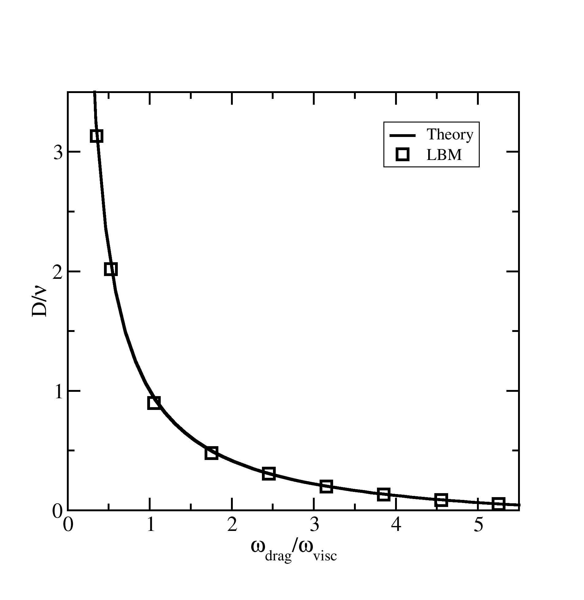
We preliminarily tested the analytical predictions of Eq. (29) for the mutual diffusion coefficient and of Eq. (35) for the electric conductivity in bulk conditions. In these tests we used mesh points and applied periodic boundary conditions. To calculate the mutual diffusion coefficient of the binary mixture we prepared the uniform system by adding a small sinusoidal concentration profile, and monitored its exponential decay, having a wavelength dependent characteristic time . The diffusion coefficient was obtained a function of and reported in Fig. 1. The agreement with the theoretical values is excellent and the method allows to appreciably decrease the diffusion coefficient. To compute the kinematic viscosity we induced a sinusoidal shear modulation of the barycentric velocity, and monitored its decay. We found that upon changing the mutual diffusion coefficient, the kinematic viscosity remains unaltered, as expected.
We next turn our attention to the charged ternary mixture. We first conducted a test to compute the electric conductivity in the bulk system subject to an uniform electric field. The density of the electrolytes is taken to be . We measured the total electric current at varying diffusivity and at constant electric field. The data reported in Fig. 2 show that the current is proportional to the diffusion coefficient , as predicted by the Drude-Lorentz formula Eq. (35).
We next analyze the transport behavior of the electrolytic solution moving in a slit channel having charged walls, under the action of a uniform electric field parallel to the walls. The flow is directed along the axis, the charged plates are aligned along the plane, with surface area , and the charged plates are separated along the z axis by . The total mesh size is . The surface charge of the walls is .
From the macroscopic arguments used to derive the Hemholtz-Smoluchowski theory [30] one expects that the mass current, does not depend on the diffusion constant. The bulk densities of the charged species are fixed by imposing the Debye length, since , and we considered the three values , and .
The total mass flow rate in the stationary state is defined:
| (39) |
By neglecting small variations of the total density with respect to the bulk value, the theoretical mass flow rate is given by [30]
| (40) |
where is the the inverse of the Debye length. The quantity is an increasing function of , explaining the results shown in Fig. 3. However, in the same plot we also notice a dependence of the mass flow rate on . This behavior is not accounted for by the Helmholtz-Smoluchowski theory, which in fact shows no dependence on the inter-species diffusivity. However, it should be borne in mind that one of the key assumptions of the theory is that the barycentric velocity locally equals the velocity of the neutral species, a condition that can be violated in the general case.
To verify such assumption, we report in Fig. 4 the differential velocity profiles of the three species and find that, when is large, the velocity of the neutral species is indistinguishable from the barycentric one. Vice versa, when the drag force is small the two velocities substantially depart from each other.
The electro-osmotic contribution to the charge flow rate displays a similar dependence on . To this purpose, we first consider the total electric current
| (41) |
and decompose it as the sum of two contributions stemming from Ohmic conduction and charge convection, , with the latter defined as
| (42) |
and again is the barycentric velocity along the flow direction. Similarly, the electro-osmotic contribution to conductivity is obtained by dividing the electro-osmotic current by the applied tension.
In the linear (Debye-Huckel) approximation, the convective contribution can be computed analytically and reads
| (43) |
The behavior of the curves in Fig. 5 is understood by noting that the number of charge carriers in the mixture is inversely proportional to [30]. Again, the electro-osmotic charge flow turns out to be an increasing function of as shown in Fig. 6, but depends on the mutual diffusivity, in particular by displaying a slight increase with . The reason for such behavior is the same as the one mentioned above.
Having different velocities between the solvent and the barycentric one at small , that is at high diffusivity, gives rise to a larger barycentric velocity. We performed a theoretical analysis of this occurrence at the level of linearized hydrodynamics starting from the kinetic equation (11). The results show a fairly good agreement with the simulations data and predict that the phenomenon is only visible at small values of . For the sake of conciseness, we will report the calculations elsewhere.
In essence, the Lattice Boltzmann algorithm, derived from the kinetic model introduced in this work, is capable not only to accurately reproduce the behavior predicted by the continuum equations of Sec. III, but also to exhibit non-trivial features of electrokinetic transport arising from the interplay of diffusion, convection and electrostatics.
V Conclusions
To summarize, we modified the BGK dynamics in order to control separately the timescales associated to concentration and momentum diffusion. The presented method is derived from microscopic considerations involving the exact treatment of the collision term in the Boltzmann equation. We replaced the microscopic expression for the inter-species frictional force, which tends to equalize the species velocities, by a simpler effective term depending on a tunable frequency . The derived equations have similarities with the ones put forward by Luo and Girimaji [31]. However, the orthogonalization procedure described here represents a key ingredient to separately control concentration and momentum diffusion.
We further implemented the equations in the context of the Lattice Boltzmann Method, and numerically verified that controlling independently the diffusivity and the kinematic viscosity for different physical models is feasible and mirrors the expected dynamics in the continuum. We applied the method to the numerical calculation of the diffusion coefficient in neutral binary mixtures and of the electric currents of ternary charged mixtures under uniform bulk conditions, finding a perfect agreement with the theoretical prediction.
Under non uniform conditions, such as those realized in a charged slit geometry, the electro-osmotic current exhibits a non-trivial behavior, since the convective contributions to the mass and charge currents display an interesting dependence on the diffusion coefficient. Such occurrence, to the best of our knowledge, was not previously reported in the literature.
We conclude with a remark concerning the relation between the present approach and the standard single relaxation, BGK description of mixtures. When the value of the tunable parameter is chosen to be equal to , on physical grounds one does not expect to observe differences between the two methods. Not only we have confirmed numerically such an occurrence, but it we also demonstrated that the kinetic equation (11) in practice reduces to the standard BGK single relaxation form in this limit.
V.1 Acknowledgments
This work was supported by the Italian Ministry of University and Research through the “Futuro in Ricerca” project RBFR12OO1G - NEMATIC.
Appendix A Hermite expansion of the kinetic equation (11)
The standard procedure to construct the LBM algorithm starting from the kinetic equation is to expand each term of the equation in the Hermite polynomial basis. It is apparent that the coefficients of the expansion of the distribution function and the collisional terms are combination of the macroscopic fields [29]. This property, together with the orthogonality of the basis set, not only guarantees that, given an expansion order , the first moments of the distribution are untouched by the truncation but also permits to control the error introduced by the evolution equation in the macroscopic fields [32, 29]. Using the Einstein convention on the repeated indices, the one particle distribution function expands as
| (44) |
where represents the k-th derivative with respect to and is a sum of products of ’s, each having one subscript from the set and one from the set [33]. From the definition, it follows that
| (45) |
In the following, we will often make use of the identities and consider the Hermite expansion up to second order of the equation
| (46) |
with
Both terms in the r.h.s. of Eq. (46) have a dependence of the type , so that
| (47) |
and
| (48) |
The force term has the following discrete representation
where . The analogous expansion of reads
| (50) | |||||
The expansion of to second order is well-known (see for example [29]), so that we report here only the projections of , to the same order. The integrals involved in the calculation of the projection of , were given before (see Eq. (47)) while for the remaining ones, we obtain:
| (51) |
Putting all together,
References
- [1] Reto B Schoch, Jongyoon Han, and Philippe Renaud. Transport phenomena in nanofluidics. Reviews of Modern Physics, 80(3):839, 2008.
- [2] Brian Kirby. Micro-and nanoscale fluid mechanics: transport in microfluidic devices. Cambridge University Press, 2010.
- [3] Jean Berthier and Pascal Silberzan. Microfluidics for biotechnology. Artech House, 2010.
- [4] Roberto Benzi, Sauro Succi, and Massimo Vergassola. The lattice boltzmann equation: theory and applications. Physics Reports, 222(3):145–197, 1992.
- [5] Sauro Succi. The lattice Boltzmann equation: for fluid dynamics and beyond. Oxford university press, 2001.
- [6] Prabhu Lal Bhatnagar, Eugene P Gross, and Max Krook. A model for collision processes in gases. i. small amplitude processes in charged and neutral one-component systems. Physical review, 94(3):511, 1954.
- [7] Shiyi Chen and Gary D Doolen. Lattice boltzmann method for fluid flows. Annual review of fluid mechanics, 30(1):329–364, 1998.
- [8] Lawrence Sirovich. Kinetic modeling of gas mixtures. Physics of Fluids (1958-1988), 5(8):908–918, 2004.
- [9] Bernard B Hamel. Kinetic model for binary gas mixtures. Physics of Fluids (1958-1988), 8(3):418–425, 2004.
- [10] Bernard B Hamel. Two-fluid hydrodynamic equations for a neutral, disparate-mass, binary mixture. Physics of Fluids (1958-1988), 9(1):12–22, 2004.
- [11] V Garzó, A Santos, and JJ Brey. A kinetic model for a multicomponent gas. Physics of Fluids A: Fluid Dynamics (1989-1993), 1(2):380–383, 1989.
- [12] Victor Sofonea and Robert F Sekerka. Bgk models for diffusion in isothermal binary fluid systems. Physica A: Statistical Mechanics and its Applications, 299(3):494–520, 2001.
- [13] Li-Shi Luo and Sharath S Girimaji. Lattice boltzmann model for binary mixtures. Physical Review E, 66(3):035301, 2002.
- [14] Zhaoli Guo and TS Zhao. Discrete velocity and lattice boltzmann models for binary mixtures of nonideal fluids. Physical Review E, 68(3):035302, 2003.
- [15] Pietro Asinari. Asymptotic analysis of multiple-relaxation-time lattice boltzmann schemes for mixture modeling. Computers & Mathematics with Applications, 55(7):1392–1407, 2008.
- [16] Pierre Lallemand and Li-Shi Luo. Theory of the lattice boltzmann method: Dispersion, dissipation, isotropy, galilean invariance, and stability. Physical Review E, 61(6):6546, 2000.
- [17] Umberto Marini Bettolo Marconi and Simone Melchionna. Kinetic theory of correlated fluids: From dynamic density functional to lattice boltzmann methods. The Journal of Chemical Physics, 131:014105, 2009.
- [18] Umberto Marini Bettolo Marconi and Simone Melchionna. Dynamics of fluid mixtures in nanospaces. The Journal of Chemical Physics, 134(6):064118–064118, 2011.
- [19] Umberto Marini Bettolo Marconi and Simone Melchionna. Phase-space approach to dynamical density functional theory. The Journal of Chemical Physics, 126:184109, 2007.
- [20] Umberto Marini Bettolo Marconi and Simone Melchionna. Multicomponent diffusion in nanosystems. The Journal of Chemical Physics, 135:044104, 2011.
- [21] Henk Van Beijeren and Matthieu H Ernst. The modified enskog equation. Physica, 68(3):437–456, 1973.
- [22] Jean-Pierre Hansen and Ian R McDonald. Theory of simple liquids. Elsevier, 1990.
- [23] James W Dufty, Andrés Santos, and J Javier Brey. Practical kinetic model for hard sphere dynamics. Physical review letters, 77(7):1270, 1996.
- [24] Andrés Santos, José M Montanero, James W Dufty, and J Javier Brey. Kinetic model for the hard-sphere fluid and solid. Physical Review E, 57(2):1644, 1998.
- [25] H Van Beijeren and MH Ernst. The modified enskog equation for mixtures. Physica, 70(2):225–242, 1973.
- [26] Umberto Marini Bettolo Marconi. Non-local kinetic theory of inhomogeneous liquid mixtures. Molecular Physics, 109(7-10):1265–1274, 2011.
- [27] Henrik Bruus. Theoretical microfluidics, volume 18. Oxford University Press, 2008.
- [28] Sydney Chapman and Thomas George Cowling. The mathematical theory of non-uniform gases: an account of the kinetic theory of viscosity, thermal conduction and diffusion in gases. Cambridge university press, 1970.
- [29] Xiaowen Shan, Xue-Feng Yuan, and Hudong Chen. Kinetic theory representation of hydrodynamics: a way beyond the navier–stokes equation. Journal of Fluid Mechanics, 550:413–441, 2006.
- [30] Jacob H Masliyah and Subir Bhattacharjee. Electrokinetic and colloid transport phenomena. John Wiley & Sons, 2006.
- [31] Li-Shi Luo and Sharath S Girimaji. Theory of the lattice boltzmann method: two-fluid model for binary mixtures. Physical Review E, 67(3):036302, 2003.
- [32] Nicos S Martys, Xiaowen Shan, and Hudong Chen. Evaluation of the external force term in the discrete boltzmann equation. Physical Review E, 58(5):6855–6857, 1998.
- [33] Harold Grad. Note on n-dimensional hermite polynomials. Communications on Pure and Applied Mathematics, 2(4):325–330, 1949.