跳到论文正文
W Papers独立论文阅读器 arXiv:1507.04825 论文正文 计算阅读时间 · 0%
引用这篇论文根据当前论文元数据生成,正式投稿前建议核对。


License: arXiv.org perpetual non-exclusive license
arXiv:1507.04825v1 [math.OC] 17 Jul 2015

HIGHER-ORDER METRIC SUBREGULARITY AND ITS APPLICATIONS11 1 This research was partly supported by the National Science Foundation under grant DMS-12092508.
BORIS S. MORDUKHOVICH22 2 Department of Mathematics, Wayne State University, Detroit, MI 48202 (boris@math.wayne.edu). and WEI OUYANG33 3 Department of Mathematics, Wayne State University, Detroit, MI 48202 (wei@wayne.edu).

Abstract. This paper is devoted to the study of metric subregularity and strong subregularity of any positive order qq for set-valued mappings in finite and infinite dimensions. While these notions have been studied and applied earlier for q=1q=1 and—to a much lesser extent—for q∈(0,1)q\in(0,1), no results are available for the case q>1q>1. We derive characterizations of these notions for subgradient mappings, develop their sensitivity analysis under small perturbations, and provide applications to the convergence rate of Newton-type methods for solving generalized equations.
Key words. variational analysis, metric subregularity and strong subregularity of higher order, Newton and quasi-Newton methods, generalized normals and subdifferentials
AMS subject classifications. 49J52, 90C30, 90C31

1 Introduction

This paper mainly concerns the study and some applications of the notions of higher-order metric subregularity and its strong subregularity counterpart. For definiteness, we use the number q>0q>0 to indicate the order/rate of the corresponding regularity under consideration. Recall first that a set-valued mapping F:X⇉YF:X\rightrightarrows Y between Banach spaces is metrically qq-regular at (better around) (x¯,y¯)∈gph​F(\bar{x},\bar{y})\in\mbox{\rm gph}\,F if there exist a number η>0\eta>0 and neighborhoods UU of x¯\bar{x} and VV of y¯\bar{y} such that

d⁡(x,F−1​(y))≤η​dq​(y,F⁡(x))​ for all ​x∈U​ and ​y∈V,d\big(x;F^{-1}(y)\big)\leq\eta\,d^{q}\big(y;F(x)\big)\;\mbox{ for all }\;x\in U\;\text{ and }\;y\in V, (1.1)

where d⁡(⋅,Ω)d(\cdot;\Omega) is the distance function associated with Ω\Omega. It has been well recognized in nonlinear and variational analysis that metric regularity (q=1q=1) and the equivalent notions of linear openness and Lipschitzian stability play an important role in optimization, control, equilibria, and various applications as documented, e.g., in the books [5, 10, 22, 26] with many references therein. On the other hand, metric regularity often fails for broad classes of parametric variational systems given by the generalized equations in the sense of Robinson [25]:

0∈f⁡(x,y)+Q⁡(y),0\in f(x,y)+Q(y), (1.2)

where ff is single-valued while Q⁡(y)=∂φ⁡(y)Q(y)=\partial\varphi(y) is a set-valued mapping of the subdifferential/normal cone type generated by nonsmooth functions; see [23] and also [2, 3, 4, 15, 29] for more details and further results in this direction. However, this phenomenon does not appear if metric regularity is replaced by a weaker property of metric subregularity of FF at (x¯,y¯)(\bar{x},\bar{y}) defined by

d⁡(x,F−1​(y¯))≤η​d​(y¯,F⁡(x))​ for all ​x∈U.d\big(x;F^{-1}(\bar{y})\big)\leq\eta\,d\big(\bar{y};F(x)\big)\;\text{ for all }\;x\in U. (1.3)

Considering ‖x−x¯‖\|x-\bar{x}\| instead of d​(x,F−1​(y¯))d(x;F^{-1}(\bar{y})) in (1.3), we get the notion of strong metric subregularity. In the aforementioned books and in an increasing number of papers, the reader can find more information about these subregularity properties, their calmness (resp. isolated calmness) equivalents for inverse mappings, as well as their various applications to optimization.

In [6, 13, 28, 30], the authors studied the notion of Hölder metric regularity, which corresponds to (1.1) with the replacement of d⁡(y,F⁡(x))d(y;F(x)) by dq​(y,F​(x))d^{q}(y;F(x)) as 0<q<10<q<1. Replacing d⁡(y¯,F⁡(x))d(\bar{y};F(x)) by dq​(y¯,F​(x))d^{q}(\bar{y};F(x)) in (1.3) as 0<q<10<q<1 gives us the notion of Hölder metric subregularity considered recently in [14, 18, 19] from different viewpoints while without its strong counterpart.

It is essential to mention that there is no sense to study metric qq-regularity of single-valued or set-valued mappings for q>1q>1, since only constant mappings satisfy this property. However, it is not the case for qq-subregularity that is equally important whenever q>0q>0 as demonstrated in this paper, where—to the best of our knowledge—the notion of qq-subregularity for q>1q>1 is studied and applied for the first time in the literature.

In what follows we investigate both notions of metric qq-subregularity and strong metric qq-subregularity for any positive qq concentrating mainly on the higher-order case of q>1q>1. In this way we derive verifiable sufficient conditions and necessary conditions for these notions of qq-subregularity in terms of appropriate generalized differential constructions of variational analysis, study their behavior with respect to perturbations, and obtain their applications to the rate of convergence of Newton’s and quasi-Newton methods for solving generalized equations.

Accordingly, we organize the rest of the paper. Section 2 contains some preliminaries from variational analysis and generalized differentiation widely used in the formulations and proofs of the main results given below. Section 3 is devoted to a detailed study of qq-subregularity of set-valued valued mappings between general Banach and Asplund spaces concentrating mainly on subdifferential mappings. In addition to deriving verifiable conditions that imply and are implied by these notions, we compare them (when appropriate) with the corresponding notions of metric regularity and provide several numerical examples illustrating the new phenomena.

Section 4 studies behavior of strong metric qq-subregularity as q≥1q\geq 1 under parameter perturbations. The obtained results, being of their own interest, allow us to establish in Section 5 the convergence rate for Newton’s and quasi-Newton methods of solving generalized equations depending on the order of the strong metric subregularity for the underlying set-valued mapping in the generalized equation under consideration. Section 6 presents concluding remarks and some directions of our future research.

Throughout the paper we use standard notation of variational analysis and generalized differentiation. Recall that, given a set-valued mapping F:X→→X∗F\colon X\;{\lower 1.0pt\hbox{$\rightarrow$}}\kern-10.0pt\hbox{\raise 2.0pt\hbox{$\rightarrow$}}\;X^{*} from the Banach space XX into its topological dual X∗X^{*} endowed with the weak∗ topology w∗w^{*}, the symbol

Lim​supx→x¯F(x):={x∗∈X∗|∃seqs. xk→x¯,xk∗→w∗x∗with xk∗∈F(xk),k∈IN}\displaystyle\displaystyle\mathop{{\rm Lim}\,{\rm sup}}_{x\to\bar{x}}F(x):=\big\{x^{*}\in X^{*}\big|\;\exists\,\mbox{seqs. }\,x_{k}\to\bar{x},\;x^{*}_{k}\stackrel{{\scriptstyle w^{*}}}{{\to}}x^{*}\;\mbox{with }x^{*}_{k}\in F(x_{k}),\;k\in I\!\!N\Big\} (1.4)

signifies the sequential Painlevé-Kuratowski outer limit of FF as x→x¯x\to\bar{x}, where I​N:={1,2,…}I\!\!N:=\{1,2,\ldots\}. Given a set Ω⊂ℝn\Omega\subset\mathbb{R}^{n} and an extended-real-valued function φ:ℝn→ℝ¯:=(−∞,∞]\varphi\colon\mathbb{R}^{n}\to\overline{\mathbb{R}}:=(-\infty,\infty] finite at x¯\bar{x}, the symbols x→Ωx¯x\stackrel{{\scriptstyle\Omega}}{{\to}}\bar{x} and x→φx¯x\stackrel{{\scriptstyle\varphi}}{{\to}}\bar{x} stand for x→x¯x\to\bar{x} with x∈Ωx\in\Omega and for x→x¯x\to\bar{x} with φ⁡(x)→φ⁡(x¯)\varphi(x)\to\varphi(\bar{x}), respectively. As usual, I​B​(x,r)=I​Br​(x)I\!\!B(x,r)=I\!\!B_{r}(x) denotes the closed ball of the space in question centered at xx with radius r>0r>0, while the symbols I​BI\!\!B and I​B∗I\!\!B^{*} signify the corresponding closed unit ball in the primal and dual spaces, respectively. Finally, given a mapping g:X→Yg\colon X\to Y between Banach spaces that is locally Lipschitzian around x¯\bar{x}, we denote

lip​g​(x¯):=lim supx,u→x¯‖g⁡(x)−g⁡(u)‖‖x−u‖.\mbox{\rm lip}\,g(\bar{x}):=\displaystyle\limsup_{x,u\to\bar{x}}\frac{\|g(x)-g(u)\|}{\|x-u\|}.

2 Generalized Differentiation

In this section we present for the reader’s convenience some basic tools of generalized differentiation widely employed in what follows. We refer to the books [5, 22, 26, 27] for more details in both finite and infinite dimensions. Since the subdifferential and normal cone constructions are used below only in Asplund spaces, we confine ourselves to their definitions on this setting. Recall that a Banach space is Asplund if each of its separable subspace has a separable dual. This class of spaces is rather large including, in particular, every reflexive Banach space.

Given φ:X→ℝ¯\varphi\colon X\to\overline{\mathbb{R}} with x¯∈dom​φ\bar{x}\in\mbox{\rm dom}\,\varphi, the regular subdifferential (known also as the presubdifferential and as the Fréchet or viscosity subdifferential) of φ\varphi at x¯\bar{x} is defined by

∂^​φ​(x¯):={v∈ℝn|lim infx→x¯φ⁡(x)−φ⁡(x¯)−⟨v,x−x¯⟩‖x−x¯‖≥0}.\displaystyle\widehat{\partial}\varphi(\bar{x}):=\Big\{v\in\mathbb{R}^{n}\Big|\;\liminf_{x\to\bar{x}}\frac{\varphi(x)-\varphi(\bar{x})-\langle v,x-\bar{x}\rangle}{\|x-\bar{x}\|}\geq 0\Big\}. (2.1)

It reduces to {∇φ​(x¯)}\{\nabla\varphi(\bar{x})\} if φ\varphi is Fréchet differentiable at x¯\bar{x} and to the subdifferential of convex analysis if φ\varphi is convex, while the set ∂^​φ​(x¯)\widehat{\partial}\varphi(\bar{x}) may often be empty for nonconvex and nonsmooth functions as, e.g., for φ⁡(x)=−|x|\varphi(x)=-|x| at x¯=0∈ℝ\bar{x}=0\in\mathbb{R}. A serious disadvantage of (2.1) is the failure of standard calculus rules required in variational analysis and its applications to optimization.

We come to the different picture while performing a limiting procedure/robust regularization over the mapping x↦∂^​φ​(x)x\mapsto\widehat{\partial}\varphi(x) as x→φx¯x\stackrel{{\scriptstyle\varphi}}{{\to}}\bar{x} vis the sequential outer limit (1.4), which gives us the (basic first-order) subdifferential of φ\varphi at x¯\bar{x} defined by

∂φ⁡(x¯):=Lim​supx→φx¯⁡∂^​φ​(x)\displaystyle\partial\varphi(\bar{x}):=\displaystyle\mathop{{\rm Lim}\,{\rm sup}}_{x\stackrel{{\scriptstyle\varphi}}{{\to}}\bar{x}}\widehat{\partial}\varphi(x) (2.2)

and known also as the general, or limiting, or Mordukhovich subdifferential. In contrast to (2.1), the set (2.2) is often nonconvex (e.g., ∂φ⁡(0)={−1,1}\partial\varphi(0)=\{-1,1\} for φ⁡(x)=−|x|\varphi(x)=-|x|) enjoying nevertheless comprehensive calculus based on variational/extremal principles of variational analysis.

3 Necessary and Sufficient Conditions for qq-Subregularity

Let us start this section with the basic definition of positive-order metric subregularity for arbitrary set-valued mappings between Banach spaces.

Definition 3.1 (metric qq-subregularity and strong qq-subregularity).

Let F:X→→YF:X\;{\lower 1.0pt\hbox{$\rightarrow$}}\kern-10.0pt\hbox{\raise 2.0pt\hbox{$\rightarrow$}}\;Y with (x¯,y¯)∈gph​F(\bar{x},\bar{y})\in\mbox{\rm gph}\,F, and let q>0q>0. We say that:

(i) FF is metrically qq-subregular at (x¯,y¯)(\bar{x},\bar{y}) if there are constants η,γ>0\eta,\gamma>0 such that

d⁡(x,F−1​(y¯))≤η​dq​(y¯,F⁡(x))​ for all ​x∈I​B​(x¯,γ)d\big(x;F^{-1}(\bar{y})\big)\leq\eta d^{q}\big(\bar{y};F(x)\big)\;\mbox{ for all }\;x\in I\!\!B(\bar{x};\gamma) (3.1)

The infimum over all constants/moduli η>0\eta>0 for which (3.1) holds with some γ>0\gamma>0 is called the exact q-subregularity bound of F at (x¯,y¯)(\bar{x},\bar{y}) and is denoted by subregq​F​(x¯,y¯)\mbox{\rm subreg}\,^{q}F(\bar{x},\bar{y}).

(ii) FF is strongly metrically qq-subregular at (x¯,y¯)(\bar{x},\bar{y}) if there are η,γ>0\eta,\gamma>0 such that

‖x−x¯‖≤η​dq​(y¯,F⁡(x))​ for all ​x∈I​B​(x¯,γ).\|x-\bar{x}\|\leq\eta d^{q}\big(\bar{y};F(x)\big)\;\mbox{ for all }\;x\in I\!\!B(\bar{x};\gamma). (3.2)

The infimum over all η>0\eta>0 for which (3.2) holds with some γ>0\gamma>0 is called the exact strong q-subregularity bound of F at (x¯,y¯)(\bar{x},\bar{y}) and is denoted by ssubregq​F​(x¯,y¯)\mbox{\rm ssubreg}\,^{q}F(\bar{x},\bar{y}).

For brevity, in what follows we omit the adjective “metric” for qq-subregularity. It is easy to see from the definitions that the strong qq-subregularity of FF at (x¯,y¯)(\bar{x},\bar{y}) implies the corresponding qq-subregularity of FF. Furthermore, the validity of q¯\bar{q}-subregularity (resp. strong q¯\bar{q}-subregularity) of FF ar (x¯,y¯)(\bar{x},\bar{y}) for the fixed number q¯>0\bar{q}>0 ensures this property for any 0<q≤q¯0<q\leq\bar{q}.

Clearly, the larger qq in the above subregularity properties the better the corresponding estimate (error bound) in (3.1) and (3.2) is. The following simple one-dimensional example shows that it makes sense to consider the qq-subregularity property of order q>1q>1, in contrast to its metric regularity counterpart of such (higher) orders, even in the case of real functions.

Example 3.2 (qq-subregularity of higher order).

Consider the continuous function f⁡(x):=|x|12f(x):=|x|^{\frac{1}{2}}, x∈ℝx\in\mathbb{R}, which is not Lipschitz continuous around x¯=0\bar{x}=0. We have

|x|≤|x12|q​for any q∈(0,2] and all x∈I​B​(0,1).|x|\leq|x^{\frac{1}{2}}|^{q}\;\mbox{for any $q\in(0,2]$ and all $x\in I\!\!B(0,1)$}.

This shows that ff is strongly qq-subregular at (0,0)(0,0) whenever q∈(0,2]q\in(0,2].

The next example is more involved, being still one-dimensional, and reveals an interesting phenomenon: a set-valued mapping may not be metrically regular around the given point while it is metrically subregular at this point with some q>1q>1. This example concerns in fact solution maps of the parametric generalized equations of type (1.2), which fails to have the metric regularity property in common situations; see Section 1.

Example 3.3 (qq-subregular but not metrically regular solution maps to parametric generalized equations).

Consider the solution map

S⁡(x)={y∈Rn| 0∈f⁡(x,y)+Q⁡(y)}\displaystyle S(x)=\big\{y\in R^{n}\big|\;0\in f(x,y)+Q(y)\big\} (3.3)

of the parametric generalized equation (1.2) with f⁡(x,y):=xf(x,y):=x and Q:ℝ→→ℝQ\colon\mathbb{R}\;{\lower 1.0pt\hbox{$\rightarrow$}}\kern-10.0pt\hbox{\raise 2.0pt\hbox{$\rightarrow$}}\;\mathbb{R} given by

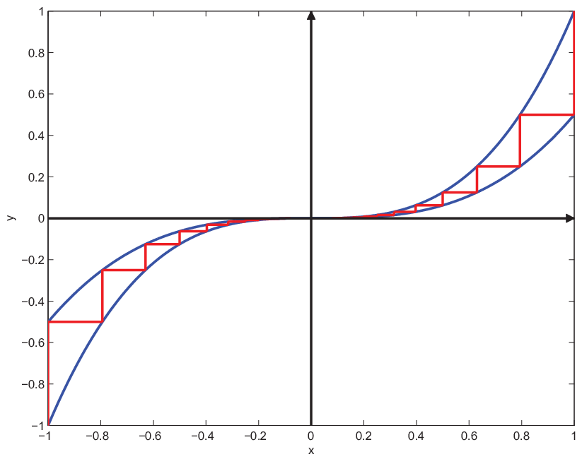
Q⁡(y):={[12k+1,12k]fory=1(23)k,12k+1fory∈(1(23)k+1,1(23)k),0fory=0,[−12k,−12k+1]fory=−1(23)k,−12k+1fory∈(−1(23)k,−1(23)k+1)\displaystyle Q(y):=\left\{\begin{array}[]{rcl}{[\frac{1}{2^{k+1}},\frac{1}{2^{k}}]}&\mbox{for}&y=\frac{1}{(\sqrt[3]{2})^{k}},\\ \frac{1}{2^{k+1}}&\mbox{for}&y\in\Big(\frac{1}{(\sqrt[3]{2})^{k+1}},\frac{1}{(\sqrt[3]{2})^{k}}\Big),\\ 0&\mbox{for}&y=0,\\ {[-\frac{1}{2^{k}},-\frac{1}{2^{k+1}}]}&\mbox{for}&y=-\frac{1}{(\sqrt[3]{2})^{k}},\\ -\frac{1}{2^{k+1}}&\mbox{for}&y\in\Big(-\frac{1}{(\sqrt[3]{2})^{k}},-\frac{1}{(\sqrt[3]{2})^{k+1}}\Big)\end{array}\right.

as depicted in Figure 1. Then SS is not metrically regular around (0,0)(0,0) while it is strongly qq-subregular of any order q∈(0,2]q\in(0,2] at this point.

Refer to caption
Figure 1: Q(y)

Indeed, the failure of metric regularity of SS in (3.3) around (0,0)(0,0) follows from more general results of [23]. Let us verify this directly for the mapping SS under consideration. Due to the form of SS in (3.3) and the well-known equivalence between metric regularity of the given mapping and the Lipschitz-like/Aubin property of its inverse (see, e.g., [22, Theorem 1.49]), it suffices to show that QQ in (3.3) is not Lipschitz-like around (0,0)(0,0). By [22, Theorem 1.41] this is equivalent to the fact that the scalar function

ρ⁡(x,y):=dist​(x,Q⁡(y))=inf{‖x−v‖|v∈Q⁡(y)}\rho(x,y):=\text{dist}\big(x;Q(y)\big)=\inf\big\{\|x-v\|\big|\;v\in Q(y)\big\}

is not locally Lipschitzian around (0,0)(0,0). To check the latter, we construct two sequences {(x1​k,y1​k)}\{(x_{1k},y_{1k})\} and {(x2​k,y2​k)}\{(x_{2k},y_{2k})\}, which converge to (0,0)(0,0) when k→∞k\rightarrow\infty as follows:

x1​k:=12k−1,y1​k:=1(23)k−1−αk,where0<αk<min{1k​2k,1(23)k−1−1(23)k};\displaystyle x_{1k}:=\frac{1}{2^{k-1}},\;y_{1k}:=\frac{1}{(\sqrt[3]{2})^{k-1}}-\alpha_{k},\hskip 10.00002pt\text{where}\hskip 10.00002pt0<\alpha_{k}<\min\Big\{\frac{1}{k2^{k}},\frac{1}{(\sqrt[3]{2})^{k-1}}-\frac{1}{(\sqrt[3]{2})^{k}}\Big\};
x2​k:=12k−1,y2​k:=1(23)k−1,k∈I​N.x_{2k}:=\frac{1}{2^{k-1}},\hskip 10.00002pty_{2k}:=\frac{1}{(\sqrt[3]{2})^{k-1}},\hskip 10.00002ptk\in I\!\!N.

Then we have the equalities

dist​(x2​k,Q⁡(y2​k))=dist​(x2​k,[12k,12k−1])=dist​(12k−1,[12k,12k−1])=0,\text{dist}(x_{2k};Q(y_{2k}))=\text{dist}\Big(x_{2k};{\Big[\frac{1}{2^{k}},\frac{1}{2^{k-1}}\Big]}\Big)=\text{dist}\Big(\frac{1}{2^{k-1}},{\Big[\frac{1}{2^{k}},\frac{1}{2^{k-1}}\Big]}\Big)=0,
dist​(x1​k,Q⁡(y1​k))=dist​(12k−1,12k)=12k,\text{dist}\big(x_{1k};Q(y_{1k})\big)=\text{dist}\Big(\frac{1}{2^{k-1}};\frac{1}{2^{k}}\Big)=\frac{1}{2^{k}},

where the last one holds due to the estimates

1(23)k<y1​k<1(23)k−1,k∈I​N.\frac{1}{(\sqrt[3]{2})^{k}}<y_{1k}<\frac{1}{(\sqrt[3]{2})^{k-1}},\hskip 10.00002ptk\in I\!\!N.

Since ‖y1​k−y2​k‖=αk≤(k​2k)−1\|y_{1k}-y_{2k}\|=\alpha_{k}\leq({k2^{k}})^{-1}, we have

‖d⁡(x1​k,Q⁡(y1​k))−d⁡(x2​k,Q⁡(y2​k))‖=12k≥k​αk=k​‖(x1​k−x2​k,y1​k−y2​k)‖,\big\|d\big(x_{1k};Q(y_{1k})\big)-d\big(x_{2k};Q(y_{2k})\big)\big\|=\frac{1}{2^{k}}\geq k\alpha_{k}=k\|(x_{1k}-x_{2k},y_{1k}-y_{2k})\|,

which indicates that ρ⁡(x,y)\rho(x,y) is not locally Lipschitzian around (0,0)(0,0) and yields therefore that the solution map SS from (3.3) is not metrically regular around (0,0)(0,0).

Now we show that SS is qq-subregular for q=2q=2 and thus for any q∈(0,2]q\in(0,2] at (0,0)(0,0). To proceed, take η=γ=1\eta=\gamma=1 and, given x∈B⁡(0,γ)x\in B(0,\gamma), find k0k_{0} so that |x|∈[12k0+1,12k0]|x|\in{[\frac{1}{2^{k_{0}+1}},\frac{1}{2^{k_{0}}}]} and the corresponding value |Q−1​(x)||Q^{-1}(x)| belongs to [1(23)k+1,1(23)k−1]{\Big[\frac{1}{(\sqrt[3]{2})^{k+1}},\frac{1}{(\sqrt[3]{2})^{k-1}}\Big]}. Notice that S−1​(0)={0}S^{-1}(0)=\{0\}, we have

d⁡(x,S−1​(0))=|x|\displaystyle d\big(x;S^{-1}(0)\big)=|x| ≤\displaystyle\leq η​d2​(0,S⁡(x))=η​(inf{‖y‖|y∈Q−1​(x)})2,x∈I​B​(0,γ),\displaystyle\eta d^{2}\big(0;S(x)\big)=\eta\big(\inf\big\{\|y\|\big|\;y\in Q^{-1}(x)\big\}\big)^{2},\hskip 10.00002ptx\in I\!\!B(0,\gamma),

due to 12k≤1(23)2​(k+1)\frac{1}{2^{k}}\leq\frac{1}{(\sqrt[3]{2})^{2}(k+1)} for any k≥2k\geq 2, which verifies the 22-subregularity of SS at (0,0)(0,0) and thus completes our justification in this example.

It is worth mentioning that the solution map (3.3) in Example 3.3 happens to be even strongly 22-subregular at (0,0)(0,0). It follows from the arguments above since S−1​(0)={0}S^{-1}(0)=\{0\} is a singleton.

Next we derive characterizations of qq-subregularity of any rate q>0q>0 for the subdifferential mappings (2.2) generated by extended-real-valued lower semicontinuous (l.s.c.) functions on Banach (sufficient conditions) and Asplund (necessary conditions) spaces. For the case of subregularity (q=1q=1) the obtained characterization reduces to [11, Theorem 3.1]. For convex functions on Banach spaces this case while concerning only local minimizers xx of ff has been independently characterized in [1, Theorem 2.1] with a weaker modulus estimate; see more discussions in [11] presented around Corollary 3.2 and also in [1, Remark 2.2] for convex and nonconvex functions with q=1q=1. In the general case of qq-subregularity the formulation and proof of the theorem below are essentially more involved following the lines of the approach in [24, Theorem 3.2] (for strong metric regularity) and of [11, Theorem 3.1] (for subregularity).

Theorem 3.4 (characterization of qq-subregularity of the basic subdifferential).

Let f:X→R¯f\colon X\rightarrow\overline{R} be l.s.c. around x¯∈dom​f\bar{x}\in\mbox{\rm dom}\,f on a Banach space XX, let x¯∗∈∂f⁡(x¯)\bar{x}^{*}\in\partial f(\bar{x}), and let qq be an arbitrary positive number. Consider the following two statements:

(i) ∂f\partial f is qq-subregular at (x¯,x¯∗)(\bar{x},\bar{x}^{*}) with modulus κ~\widetilde{\kappa} and there exist numbers γ>0\gamma>0 and r∈(0,q/κ)r\in(0,q/\kappa) with κ:=q​κ~1q\kappa:=q\widetilde{\kappa}^{\frac{1}{q}} such that

f⁡(x)≥f⁡(x¯)+⟨x¯∗,x−x¯⟩−q​r1+q​d1+qq​(x,(∂f)−1​(x¯∗))​ for all ​x∈I​B​(x¯,γ).f(x)\geq f(\bar{x})+\langle{\bar{x}}^{*},x-\bar{x}\rangle-\frac{qr}{1+q}d^{\frac{1+q}{q}}\big(x;(\partial f)^{-1}(\bar{x}^{*})\big)\;\mbox{ for all }\;x\in I\!\!B(\bar{x},\gamma). (3.5)

(ii) There are two positive numbers α\alpha and η\eta such that

f⁡(x)≥f⁡(x¯)+⟨x¯∗,x−x¯⟩+q​α1+q​d1+qq​(x,(∂f)−1​(x¯∗))​ for all ​x∈I​B​(x¯,η).f(x)\geq f(\bar{x})+\langle{\bar{x}}^{*},x-\bar{x}\rangle+\frac{q\alpha}{1+q}d^{\frac{1+q}{q}}\big(x;(\partial f)^{-1}(\bar{x}^{*})\big)\;\mbox{ for all }\;x\in I\!\!B(\bar{x},\eta). (3.6)

Then we have (ii)⟹\Longrightarrow(i) provided that there is β∈(0,α)\beta\in(0,\alpha) with

f⁡(u)≥f⁡(x)+⟨x∗,u−x⟩−q​β1+q​d1+qq​(x,(∂f)−1​(x¯∗))f(u)\geq f(x)+\langle{x}^{*},u-x\rangle-\frac{q\beta}{1+q}d^{\frac{1+q}{q}}\big(x,(\partial f)^{-1}(\bar{x}^{*})\big) (3.7)

whenever (u,x¯∗),(x,x∗)∈(gph​∂f)∩I​B​((x¯,x¯∗),η+(q​η1+q)1q)(u,{\bar{x}}^{*}),(x,x^{*})\in(\mbox{\rm gph}\,\partial f)\cap I\!\!B\big((\bar{x},{\bar{x}}^{*}),\eta+(\frac{q\eta}{1+q})^{\frac{1}{q}}\big). Conversely, we have (i)⟹\Longrightarrow(ii) for any fixed α∈(0,q/κ)\alpha\in(0,q/\kappa) provided that the space XX is Asplund.

Proof. Let us first justify implication (ii)⟹\Longrightarrow(i) in the case of the general Banach space XX assuming condition (3.7) with some β∈(0,α)\beta\in(0,\alpha). Since (3.6) clearly yields (3.5), we will arrive at (i) by showing that there exists a number κ~>0\widetilde{\kappa}>0 such that

d⁡(x,(∂f)−1​(x¯∗))≤κ~​dq​(x¯∗,∂f⁡(x))​ for all ​x∈I​B​(x¯,η​q/1+q).d\big(x;(\partial f)^{-1}(\bar{x}^{*})\big)\leq\widetilde{\kappa}d^{q}\big(\bar{x}^{*};\partial f(x)\big)\;\mbox{ for all }\;x\in I\!\!B\big(\bar{x},\eta q/1+q\big). (3.8)

To proceed, fix x∈I​B​(x¯,η​q/1+q)x\in I\!\!B(\bar{x},\eta q/1+q). Pick any u∈(∂f)−1​(x¯∗)u\in(\partial f)^{-1}(\bar{x}^{*}) with ‖x−u‖≤q−1​‖x−x¯‖\|x-u\|\leq q^{-1}\|x-\bar{x}\| and get

‖u−x¯‖≤‖u−x‖+‖x−x¯‖≤η.\|u-\bar{x}\|\leq\|u-x\|+\|x-\bar{x}\|\leq\eta.

Then it follows from (3.7) the estimates

f⁡(x¯)≥f⁡(u)+⟨x¯∗,x¯−u⟩−β​q1+q​d1+qq​(u,(∂f)−1​(x¯∗))≥f⁡(u)+⟨x¯∗,x¯−u⟩,\displaystyle f(\bar{x})\geq f(u)+\langle{\bar{x}}^{*},\bar{x}-u\rangle-\frac{\beta q}{1+q}d^{\frac{1+q}{q}}\big(u;(\partial f)^{-1}(\bar{x}^{*})\big)\geq f(u)+\langle\bar{x}^{*},\bar{x}-u\rangle, (3.9)

which ensure in turn that for any such uu and x∗∈∂f⁡(x)∩I​B​(x¯∗,[η​q/(1+q)]1q)x^{*}\in\partial f(x)\cap I\!\!B(\bar{x}^{*},[\eta q/(1+q)]^{\frac{1}{q}}) we have

⟨x∗−x¯∗,x−u⟩\displaystyle\langle x^{*}-\bar{x}^{*},x-u\rangle =\displaystyle= ⟨x∗,x−u⟩+⟨x¯∗,u−x¯⟩−⟨x¯∗,x−x¯⟩\displaystyle\langle x^{*},x-u\rangle+\langle\bar{x}^{*},u-\bar{x}\rangle-\langle\bar{x}^{*},x-\bar{x}\rangle
≥\displaystyle\geq f⁡(x)−f⁡(u)−β​q1+q​dq+1q​(x,(∂f)−1​(x¯∗))+f⁡(u)−f⁡(x¯)−⟨x¯∗,x−x¯⟩\displaystyle f(x)-f(u)-\frac{\beta q}{1+q}d^{\frac{q+1}{q}}\big(x;(\partial f)^{-1}(\bar{x}^{*})\big)+f(u)-f(\bar{x})-\langle\bar{x}^{*},x-\bar{x}\rangle
=\displaystyle= f⁡(x)−f⁡(x¯)−⟨x¯∗,x−x¯⟩−β​q1+q​dq+1q​(x,(∂f)−1​(x¯∗))\displaystyle f(x)-f(\bar{x})-\langle\bar{x}^{*},x-\bar{x}\rangle-\frac{\beta q}{1+q}d^{\frac{q+1}{q}}\big(x;(\partial f)^{-1}(\bar{x}^{*})\big)
≥\displaystyle\geq q⁡(α−β)q+1​dq+1q​(x,(∂f)−1​(x¯∗)),\displaystyle\frac{q(\alpha-\beta)}{q+1}d^{\frac{q+1}{q}}\big(x;(\partial f)^{-1}(\bar{x}^{*})\big),

where the first inequality follows from (3.7) and (3.9) while the second one from (3.6). Thus

‖x∗−x¯∗‖⋅‖x−u‖≥q⁡(α−β)q+1​d1+qq​(x,(∂f)−1​(x¯∗)),\|x^{*}-\bar{x}^{*}\|\cdot\|x-u\|\geq\frac{q(\alpha-\beta)}{q+1}d^{\frac{1+q}{q}}\big(x;(\partial f)^{-1}(\bar{x}^{*})\big),

which gives us the estimate

‖x∗−x¯∗‖​d​(x,(∂f)−1​(x¯∗))≥q⁡(α−β)q+1​dq+1q​(x,(∂f)−1​(x¯∗))\|x^{*}-\bar{x}^{*}\|d\big(x;(\partial f)^{-1}(\bar{x}^{*})\big)\geq\frac{q(\alpha-\beta)}{q+1}d^{\frac{q+1}{q}}\big(x;(\partial f)^{-1}(\bar{x}^{*})\big)

due to the arbitrary choice of u∈(∂f)−1​(x¯∗)u\in(\partial f)^{-1}(\bar{x}^{*}) with ‖x−u‖≤1q​‖x−x¯‖≤η1+q\|x-u\|\leq\frac{1}{q}\|x-\bar{x}\|\leq\frac{\eta}{1+q}. Hence

‖x∗−x¯∗‖≥q⁡(α−β)q+1​d1q​(x,(∂f)−1​(x¯∗))​ for all ​x∗∈∂f⁡(x)∩I​B​(x¯∗,[η​q/(1+q)]1q).\|x^{*}-\bar{x}^{*}\|\geq\frac{q(\alpha-\beta)}{q+1}d^{\frac{1}{q}}\big(x;(\partial f)^{-1}(\bar{x}^{*})\big)\;\mbox{ for all }\;x^{*}\in\partial f(x)\cap I\!\!B\big(\bar{x}^{*},[\eta q/(1+q)]^{\frac{1}{q}}\big). (3.10)

If d⁡(x¯∗,∂f⁡(x))≤(η​q/1+q)1qd(\bar{x}^{*};\partial f(x))\leq(\eta q/1+q)^{\frac{1}{q}}, we deduce from (3.10) that

d⁡(x¯∗,∂f⁡(x))≥q⁡(α−β)q+1​d1q​(x,(∂f)−1​(x¯∗))​ for all ​x∈I​B​(x¯,η​q/(1+q)),d\big(\bar{x}^{*};\partial f(x)\big)\geq\frac{q(\alpha-\beta)}{q+1}d^{\frac{1}{q}}\big(x;(\partial f)^{-1}(\bar{x}^{*})\big)\;\mbox{ for all }\;x\in I\!\!B(\bar{x},\eta q/(1+q)\big),

which justifies (3.8) with κ~:=[(1+q)/(q(α−β)]q\widetilde{\kappa}:=[(1+q)/(q(\alpha-\beta)]^{q}. In the remaining case of d⁡(x¯∗,∂f⁡(x))>(η​q/1+q)1qd(\bar{x}^{*};\partial f(x))>(\eta q/1+q)^{\frac{1}{q}} we obviously have the estimates

d⁡(x,(∂f)−1​(x¯∗))≤‖x−x¯‖≤η​q1+q<dq​(x¯∗,∂f⁡(x)),d\big(x;(\partial f)^{-1}(\bar{x}^{*})\big)\leq\|x-\bar{x}\|\leq\frac{\eta q}{1+q}<d^{q}\big(\bar{x}^{*};\partial f(x)\big),

which also justify (3.8) is and thus completes the proof of implication (ii)⟹\Longrightarrow(i).

Next we verify the converse (i)⟹\Longrightarrow(ii) assuming that XX is Asplund. Arguing by contradiction, suppose that (i) holds while property (3.6) is not satisfied whenever α,η>0\alpha,\eta>0. Choose

0<21+qq1+q<a<∞0<\frac{2^{\frac{1+q}{q}}}{1+q}<a<\infty

and pick θ\theta from the interval (2−qq⁡(1+q),12)\big(\frac{2^{-q}}{q(1+q)},\frac{1}{2}\big), which ensures that θ+1θq​aq​(1+q)q<1\theta+\frac{1}{\theta^{q}a^{q}(1+q)^{q}}<1. Now we claim that there exists a positive number ν\nu satisfying

f⁡(x)≥f⁡(x¯)+⟨x¯∗,x−x¯⟩+q−(a​q+1)​κ​ra⁡(1+q)​κ​d1+qq​(x,(∂f)−1​(x¯∗))​ for all ​x∈I​B​(x¯,ν).f(x)\geq f(\bar{x})+\langle\bar{x}^{*},x-\bar{x}\rangle+\frac{q-(aq+1)\kappa r}{a(1+q)\kappa}d^{\frac{1+q}{q}}\big(x;(\partial f)^{-1}(\bar{x}^{*})\big)\;\mbox{ for all }\;x\in I\!\!B(\bar{x},\nu). (3.11)

Indeed, otherwise there is a sequence xk→x¯{x_{k}}\rightarrow\bar{x} such that

f⁡(xk)<f⁡(x¯)+⟨x¯∗,xk−x¯⟩+q−(a​q+1)​κ​ra⁡(1+q)​κ​d1+qq​(xk,(∂f)−1​(x¯∗)),k∈I​N.f(x_{k})<f(\bar{x})+\langle{\bar{x}}^{*},x_{k}-\bar{x}\rangle+\frac{q-(aq+1)\kappa r}{a(1+q)\kappa}d^{\frac{1+q}{q}}\big(x_{k};(\partial f)^{-1}(\bar{x}^{*})\big),\hskip 10.00002ptk\in I\!\!N.

This together with (3.5) implies that all xkx_{k} lie outside of (∂f)−1​(x¯∗)(\partial f)^{-1}(\bar{x}^{*}). Consequently we have

infx∈I​B​(x¯,γ){f⁡(x)−⟨x¯∗,x−x¯⟩+q​r1+q​d1+qq​(x,(∂f)−1​(x¯∗))}≥f⁡(x¯)>f⁡(xk)−⟨x¯∗,xk−x¯⟩+q​r1+q​d1+qq​(xk,(∂f)−1​(x¯∗))−q−κ​ra⁡(1+q)​κ​d1+qq​(xk,(∂f)−1​(x¯∗)).\displaystyle\begin{array}[]{ll}&\displaystyle\inf_{x\in I\!\!B(\bar{x},\gamma)}\Big\{f(x)-\langle{\bar{x}}^{*},x-\bar{x}\rangle+\frac{qr}{1+q}d^{\frac{1+q}{q}}\big(x;(\partial f)^{-1}(\bar{x}^{*})\big)\Big\}\geq f(\bar{x})\\ &\displaystyle>f(x_{k})-\langle{\bar{x}}^{*},x_{k}-\bar{x}\rangle+\frac{qr}{1+q}d^{\frac{1+q}{q}}\big(x_{k};(\partial f)^{-1}(\bar{x}^{*})\big)-\frac{q-\kappa r}{a(1+q)\kappa}d^{\frac{1+q}{q}}\big(x_{k};(\partial f)^{-1}(\bar{x}^{*})\big).\end{array}

Denote ϵk:=(q−κ​ra⁡(1+q)​κ)​d1+qq​(xk,(∂f)−1​(x¯∗))↓0\epsilon_{k}:=\big(\frac{q-\kappa r}{a(1+q)\kappa}\big)d^{\frac{1+q}{q}}\big(x_{k};(\partial f)^{-1}(\bar{x}^{*})\big)\downarrow 0 as k→∞k\to\infty and define the function

g⁡(x):=f⁡(x)−⟨x¯∗,x−x¯⟩+q​r1+q​d1+qq​(x,(∂f)−1​(x¯∗)),x∈X.g(x):=f(x)-\langle{\bar{x}}^{*},x-\bar{x}\rangle+\frac{qr}{1+q}d^{\frac{1+q}{q}}\big(x;(\partial f)^{-1}(\bar{x}^{*})\big),\hskip 10.00002ptx\in X.

It follows from (3) that g⁡(xk)<infx∈I​B​(x¯,γ)g⁡(x)+ϵkg(x_{k})<\inf_{x\in I\!\!B(\bar{x},\gamma)}g(x)+\epsilon_{k}. Applying Ekeland’s variational principle (see, e.g., [22, Theorem 2.26]) to the function g+δI​B​(x¯,γ)g+\delta_{I\!\!B(\bar{x},\gamma)} with λk:=θ​d​(xk,(∂f)−1​(x¯∗))\lambda_{k}:=\theta d\big(x_{k};(\partial f)^{-1}(\bar{x}^{*})\big) ensures the existence of a new sequence x^k\widehat{x}_{k} satisfying ‖x^k−xk‖≤λk\|\widehat{x}_{k}-x_{k}\|\leq\lambda_{k} and such that for each k∈I​Nk\in I\!\!N we have x^k∈int​I​B​(x¯,γ)\widehat{x}_{k}\in\text{int}I\!\!B(\bar{x},\gamma) (due to xk→x¯x_{k}\rightarrow\bar{x} and λk↓0\lambda_{k}\downarrow 0 as k→∞k\to\infty) and that

g⁡(x^k)<g⁡(x)+ϵkλk​‖x−x^k‖​ for all ​x∈I​B​(x¯,γ).g(\widehat{x}_{k})<g(x)+\frac{\epsilon_{k}}{\lambda_{k}}\|x-\widehat{x}_{k}\|\;\mbox{ for all }\;x\in I\!\!B(\bar{x},\gamma).

Employing the Fermat stationary rule in the above optimization problem and then using the subdifferential sum rule held in Asplund spaces by [22, Theorem 3.41], we arrive at

0\displaystyle 0 ∈\displaystyle\in ∂(g(⋅)+ϵkλk∥⋅−x^∥)(x^k)\displaystyle\partial\Big(g(\cdot)+\frac{\epsilon_{k}}{\lambda_{k}}\|\cdot-\widehat{x}\|\Big)(\widehat{x}_{k})
⊂\displaystyle\subset −x¯∗+∂f⁡(x^k)+ϵkλk​I​B∗+q​r1+q​∂d1+qq​(⋅,(∂f)−1​(x¯∗))​(x^k)\displaystyle-{\bar{x}}^{*}+\partial f(\widehat{x}_{k})+\frac{\epsilon_{k}}{\lambda_{k}}I\!\!B^{*}+\frac{qr}{1+q}\partial d^{\frac{1+q}{q}}\big(\cdot;(\partial f)^{-1}(\bar{x}^{*})\big)(\widehat{x}_{k})
⊂\displaystyle\subset −x¯∗+∂f⁡(x^k)+(r​d1q​(x^k,(∂f)−1​(x¯∗))+ϵkλk)​I​B∗.\displaystyle-{\bar{x}}^{*}+\partial f(\widehat{x}_{k})+\Big(rd^{\frac{1}{q}}\big(\widehat{x}_{k};(\partial f)^{-1}(\bar{x}^{*})\big)+\frac{\epsilon_{k}}{\lambda_{k}}\Big)I\!\!B^{*}.

Combining this with the metric q-subregularity property of ∂f\partial f at (x¯,x¯∗)(\bar{x},{\bar{x}}^{*}) ensures the estimates

d1q​(x^k,(∂f)−1​(x¯∗))≤κq​d​(x¯∗,∂f⁡(x^k))≤κq​(r​d1q​(x^k,(∂f)−1​(x¯∗))+ϵkλk)d^{\frac{1}{q}}\big(\widehat{x}_{k};(\partial f)^{-1}(\bar{x}^{*})\big)\leq\frac{\kappa}{q}d\big(\bar{x}^{*};\partial f(\widehat{x}_{k})\big)\leq\frac{\kappa}{q}\Big(rd^{\frac{1}{q}}\big(\widehat{x}_{k};(\partial f)^{-1}(\bar{x}^{*})\big)+\frac{\epsilon_{k}}{\lambda_{k}}\Big)

for all k∈I​Nk\in I\!\!N sufficiently large. Hence for such numbers kk we get the inequality

(1−κ​rq)​d1q​(x^k,(∂f)−1​(x¯∗))≤κq​ϵkλk.\Big(1-\frac{\kappa r}{q}\Big)d^{\frac{1}{q}}\big(\widehat{x}_{k};(\partial f)^{-1}(\bar{x}^{*})\big)\leq\frac{\kappa}{q}\frac{\epsilon_{k}}{\lambda_{k}}.

This allows us to successively deduce that

(1−κ​rq)q​d​(xk,(∂f)−1​(x¯∗))\displaystyle\Big(1-\frac{\kappa r}{q}\Big)^{q}d\big(x_{k};(\partial f)^{-1}(\bar{x}^{*})\big) ≤\displaystyle\leq (1−κ​rq)q​‖x^k−xk‖+(1−κ​rq)q​d​(x^k,(∂f)−1​(x¯∗))\displaystyle\Big(1-\frac{\kappa r}{q}\Big)^{q}\|\widehat{x}_{k}-x_{k}\|+\Big(1-\frac{\kappa r}{q}\Big)^{q}d\big(\widehat{x}_{k};(\partial f)^{-1}(\bar{x}^{*})\big)
≤\displaystyle\leq (1−κ​rq)q​λk+(κ​ϵkq​λk)q\displaystyle\Big(1-\frac{\kappa r}{q}\Big)^{q}\lambda_{k}+\Big(\frac{\kappa\epsilon_{k}}{q\lambda_{k}}\Big)^{q}
≤\displaystyle\leq (1−κ​rq)q​d​(xk,(∂f)−1​(x¯∗))​(θ+1aq​θq​(q+1)q)\displaystyle\Big(1-\frac{\kappa r}{q}\Big)^{q}d\big(x_{k};(\partial f)^{-1}(\bar{x}^{*})\big)\Big(\theta+\frac{1}{a^{q}\theta^{q}(q+1)^{q}}\Big)
<\displaystyle< (1−κ​rq)q​d​(xk,(∂f)−1​(x¯∗)),\displaystyle\Big(1-\frac{\kappa r}{q}\Big)^{q}d\big(x_{k};(\partial f)^{-1}(\bar{x}^{*})\big),

where the last strict inequality follows from our choices of aa and θ\theta. Thus we arrive at the obvious contradiction, which justifiers our claim in (3.11). We conclude therefore that q−(a​q+1)​κ​r≤0q-(aq+1)\kappa r\leq 0.

Define now the real number

r1:=a​q+1q​κ​r−1a​κ∈[0,q/κ)r_{1}:=\frac{\frac{aq+1}{q}\kappa r-1}{a\kappa}\in\big[0,q/\kappa\big)

and observe that inequality (3.11) can be transformed into (3.5) with replacing rr by r1r_{1} and γ\gamma by ν\nu, respectively. Consequently there is some real number ν1\nu_{1} such that

f⁡(x)≥f⁡(x¯)+⟨x¯∗,x−x¯⟩+q−(a​q+1)​κ​r1a⁡(1+q)​κ​d1+qq​(x,(∂f)−1​(x¯∗))​ for all ​x∈I​B​(x¯,ν1).f(x)\geq f(\bar{x})+\langle{\bar{x}}^{*},x-\bar{x}\rangle+\frac{q-(aq+1)\kappa r_{1}}{a(1+q)\kappa}d^{\frac{1+q}{q}}\big(x;(\partial f)^{-1}(\bar{x}^{*})\big)\;\mbox{ for all }\;x\in I\!\!B(\bar{x},\nu_{1}).

As before, we get the inequality κ​r1>qa​q+1\kappa r_{1}>\frac{q}{aq+1}, or equivalently κ​r>qa​q+1+a​q2(a​q+1)2\kappa r>\frac{q}{aq+1}+\frac{aq^{2}}{(aq+1)^{2}}. Defining

r2:=a​q+1q​κ​r1−1a​κ∈[0,q/κ)r_{2}:=\frac{\frac{aq+1}{q}\kappa r_{1}-1}{a\kappa}\in\big[0,q/\kappa\big)

and proceeding in the same way as above lead us to the inequality κ​r>qa​q+1+a​q2(a​q+1)2+a2​q3(a​q+1)3\kappa r>\frac{q}{aq+1}+\frac{aq^{2}}{(aq+1)^{2}}+\frac{a^{2}q^{3}}{(aq+1)^{3}}. Then we get by induction the progressively stronger bounds

κ​r>qa​q+1+a​q2(a​q+1)2+…+ak−1​qk(a​q+1)k=q⁡(1−(a​qa​q+1)k)​ for all ​k∈I​N.\kappa r>\frac{q}{aq+1}+\frac{aq^{2}}{(aq+1)^{2}}+\ldots+\frac{a^{k-1}q^{k}}{(aq+1)^{k}}=q\Big(1-\Big(\frac{aq}{aq+1}\Big)^{k}\Big)\;\mbox{ for all }\;k\in I\!\!N.

Letting k→∞k\rightarrow\infty gives us κ​r>q\kappa r>q, which is a contradiction. Therefore there exist real numbers α,η>0\alpha,\eta>0 such that inequality (3.6) is satisfied.

To justify (ii), we verify now that α\alpha may be chosen arbitrarily close to q/κq/\kappa while being smaller than this number. It suffices to consider the case of α<q/κ\alpha<q/\kappa. Take a~,θ~>0\widetilde{a},\widetilde{\theta}>0 such that

q​21qa~​(1+q)<12,θ~∈(21qa~​(1+q),12), and so ​θ~+(qθ~​a~​(1+q))q<1.\frac{q2^{\frac{1}{q}}}{\widetilde{a}(1+q)}<\frac{1}{2},\hskip 10.00002pt\widetilde{\theta}\in\Big(\frac{2^{\frac{1}{q}}}{\widetilde{a}(1+q)},\frac{1}{2}\Big),\;\mbox{ and so }\;\widetilde{\theta}+\Big(\frac{q}{\widetilde{\theta}\widetilde{a}(1+q)}\Big)^{q}<1.

Given α,η>0\alpha,\eta>0 for which (3.6) holds, let us prove the existence μ>0\mu>0 such that

f⁡(x)≥f⁡(x¯)+⟨x¯∗,x−x¯⟩+q⁡(q+(a~−1)​α​κ)a~​(1+q)​κ​d1+qq​(x,(∂f)−1​(x¯∗))​ for all ​x∈I​B​(x¯,μ).f(x)\geq f(\bar{x})+\langle{\bar{x}}^{*},x-\bar{x}\rangle+\frac{q(q+(\widetilde{a}-1)\alpha\kappa)}{\widetilde{a}(1+q)\kappa}d^{\frac{1+q}{q}}\big(x;(\partial f)^{-1}(\bar{x}^{*})\big)\;\mbox{ for all }\;x\in I\!\!B(\bar{x},\mu). (3.15)

We just sketch the proof of (3.15) observing that it is similar to the proof of (3.11) given above. Arguing by contradiction, find a sequence of uk→x¯u_{k}\rightarrow\bar{x} so that

f⁡(uk)<f⁡(x¯)+⟨x¯∗,uk−x¯⟩+q⁡(q+(a~−1)​α​κ)a~​(1+q)​κ​d1+qq​(uk,(∂f)−1​(x¯∗)),k∈I​N.f(u_{k})<f(\bar{x})+\langle{\bar{x}}^{*},u_{k}-\bar{x}\rangle+\frac{q(q+(\widetilde{a}-1)\alpha\kappa)}{\widetilde{a}(1+q)\kappa}d^{\frac{1+q}{q}}\big(u_{k};(\partial f)^{-1}(\bar{x}^{*})\big),\hskip 10.00002ptk\in I\!\!N.

This gives us together with (3.6) that

infx∈I​B​(x¯,η){f⁡(x)−⟨x¯∗,x−x¯⟩−q​α1+q​d1+qq​(x,(∂f)−1​(x¯∗))}≥f⁡(x¯)>f⁡(uk)−⟨x¯∗,uk−x¯⟩−q​α1+q​d1+qq​(uk,(∂f)−1​(x¯∗))−q⁡(q−κ​α)a~​(1+q)​κ​d1+qq​(uk,(∂f)−1​(x¯∗)).\displaystyle\begin{array}[]{ll}&\displaystyle\inf_{x\in I\!\!B(\bar{x},\eta)}\Big\{f(x)-\langle{\bar{x}}^{*},x-\bar{x}\rangle-\frac{q\alpha}{1+q}d^{\frac{1+q}{q}}\big(x;(\partial f)^{-1}(\bar{x}^{*})\big)\Big\}\geq f(\bar{x})\\ &\displaystyle>f(u_{k})-\langle{\bar{x}}^{*},u_{k}-\bar{x}\rangle-\frac{q\alpha}{1+q}d^{\frac{1+q}{q}}\big(u_{k};(\partial f)^{-1}(\bar{x}^{*})\big)-\frac{q(q-\kappa\alpha)}{\widetilde{a}(1+q)\kappa}d^{\frac{1+q}{q}}\big(u_{k};(\partial f)^{-1}(\bar{x}^{*})\big).\end{array}

Denote further νk:=q⁡(q−κ​α)a~​(1+q)​κ​d1+qq​(uk,(∂f)−1​(x¯∗))↓0\nu_{k}:=\frac{q(q-\kappa\alpha)}{\widetilde{a}(1+q)\kappa}d^{\frac{1+q}{q}}\big(u_{k};(\partial f)^{-1}(\bar{x}^{*})\big)\downarrow 0 as k→∞k\to\infty and consider the function

h⁡(x):=f⁡(x)−⟨x¯∗,x−x¯⟩−q​α1+q​d1+qq​(x,(∂f)−1​(x¯∗)),x∈X,h(x):=f(x)-\langle{\bar{x}}^{*},x-\bar{x}\rangle-\frac{q\alpha}{1+q}d^{\frac{1+q}{q}}\big(x;(\partial f)^{-1}(\bar{x}^{*})\big),\hskip 10.00002ptx\in X,

for which we have h⁡(uk)<infx∈I​B​(x¯,η)h⁡(x)+νkh(u_{k})<\inf_{x\in I\!\!B(\bar{x},\eta)}h(x)+\nu_{k} whenever k∈I​Nk\in I\!\!N. Applying Ekeland’s variational principle to the function h+δI​B​(x¯,η)h+\delta_{I\!\!B(\bar{x},\eta)} with ρk:=θ~​d​(uk,(∂f)−1​(x¯∗))\rho_{k}:=\widetilde{\theta}d(u_{k};(\partial f)^{-1}(\bar{x}^{*})) ensures the existence of a new sequence {u^k}\{\widehat{u}_{k}\} satisfying ‖u^k−uk‖≤ρk\|\widehat{u}_{k}-u_{k}\|\leq\rho_{k} and such that u^k∈int​I​B​(x¯,η)\widehat{u}_{k}\in\text{int}\,I\!\!B(\bar{x},\eta) with

h⁡(u^k)<h⁡(x)+νkρk​‖x−u^k‖​ for all ​x∈I​B​(x¯,γ),k∈I​N.h(\widehat{u}_{k})<h(x)+\frac{\nu_{k}}{\rho_{k}}\|x-\widehat{u}_{k}\|\;\mbox{ for all }\;x\in I\!\!B(\bar{x},\gamma),\;k\in I\!\!N.

By the calculus rules as above we get the inclusions

0∈∂(h(⋅)+νkρk∥⋅−x^∥)(u^k)⊂−x¯∗+∂f(u^k)+(αd1q(u^k;(∂f)−1(x¯∗))+νkρk)IB∗,0\in\partial\Big(h(\cdot)+\frac{\nu_{k}}{\rho_{k}}\|\cdot-\widehat{x}\|\Big)(\widehat{u}_{k})\subset-{\bar{x}}^{*}+\partial f(\widehat{u}_{k})+\Big(\alpha d^{\frac{1}{q}}\big(\widehat{u}_{k};(\partial f)^{-1}(\bar{x}^{*})\big)+\frac{\nu_{k}}{\rho_{k}}\Big)I\!\!B^{*},

which ensure together with the qq-subregularity of ∂f\partial f at (x¯,x¯∗)(\bar{x},{\bar{x}}^{*}) that

d1q​(x^k,(∂f)−1​(x¯∗))≤κq​d​(x¯∗,∂f⁡(x^k))≤κq​(α​d1q​(u^k,(∂f)−1​(x¯∗))+νkρk)d^{\frac{1}{q}}\big(\widehat{x}_{k};(\partial f)^{-1}(\bar{x}^{*})\big)\leq\frac{\kappa}{q}d\big(\bar{x}^{*},\partial f(\widehat{x}_{k})\big)\leq\frac{\kappa}{q}\Big(\alpha d^{\frac{1}{q}}\big(\widehat{u}_{k};(\partial f)^{-1}(\bar{x}^{*})\big)+\frac{\nu_{k}}{\rho_{k}}\Big)

for all k∈I​Nk\in I\!\!N sufficiently large. Thus for such kk we arrive at the estimate

(1−κ​αq)​d1q​(u^k,(∂f)−1​(x¯∗))≤κq​νkρk.\Big(1-\frac{\kappa\alpha}{q})d^{\frac{1}{q}}\big(\widehat{u}_{k};(\partial f)^{-1}(\bar{x}^{*})\big)\leq\frac{\kappa}{q}\frac{\nu_{k}}{\rho_{k}}.

This allows us to successively deduce that

(1−κ​αq)q​d​(uk,(∂f)−1​(x¯∗))\displaystyle\Big(1-\frac{\kappa\alpha}{q}\Big)^{q}d\big(u_{k};(\partial f)^{-1}(\bar{x}^{*})\big) ≤\displaystyle\leq (1−κ​αq)q​‖u^k−uk‖+(1−κ​αq)q​d​(u^k,(∂f)−1​(x¯∗))\displaystyle\Big(1-\frac{\kappa\alpha}{q}\Big)^{q}\|\widehat{u}_{k}-u_{k}\|+\Big(1-\frac{\kappa\alpha}{q}\Big)^{q}d\big(\widehat{u}_{k};(\partial f)^{-1}(\bar{x}^{*})\big)
≤\displaystyle\leq (1−κ​αq)q​ρk+(κ​νkq​ρk)q\displaystyle\Big(1-\frac{\kappa\alpha}{q}\Big)^{q}\rho_{k}+\Big(\frac{\kappa\nu_{k}}{q\rho_{k}}\Big)^{q}
≤\displaystyle\leq (1−κ​αq)q​d​(uk,(∂f)−1​(x¯∗))​(θ~+(qa~​θ~​(q+1))q)\displaystyle\Big(1-\frac{\kappa\alpha}{q}\Big)^{q}d\big(u_{k};(\partial f)^{-1}(\bar{x}^{*})\big)\Big(\widetilde{\theta}+\Big(\frac{q}{\widetilde{a}\widetilde{\theta}(q+1)}\Big)^{q}\Big)
<\displaystyle< (1−κ​αq)q​d​(uk,(∂f)−1​(x¯∗)),\displaystyle\Big(1-\frac{\kappa\alpha}{q}\Big)^{q}d\big(u_{k};(\partial f)^{-1}(\bar{x}^{*})\big),

which is a contradiction justifying the existence of μ>0\mu>0 such that (3.15) holds.

In the last part of the proof we define the number

α1:=(q+(a~−1)​α​κ)a~​κ∈(0,q/κ)\alpha_{1}:=\frac{(q+(\widetilde{a}-1)\alpha\kappa)}{\widetilde{a}\kappa}\in\big(0,q/\kappa\big)

and observe that (3.15) yields (3.6) with this number α1\alpha_{1} and η=μ\eta=\mu from (3.15). Then proceeding as above allows us to find μ1>0\mu_{1}>0 such that

f⁡(x)≥f⁡(x¯)+⟨x¯∗,x−x¯⟩+q⁡(q+(a~−1)​α1​κ)a~​(1+q)​κ​d1+qq​(x,(∂f)−1​(x¯∗))​ for all ​x∈I​B​(x¯,μ1).f(x)\geq f(\bar{x})+\langle{\bar{x}}^{*},x-\bar{x}\rangle+\frac{q(q+(\widetilde{a}-1)\alpha_{1}\kappa)}{\widetilde{a}(1+q)\kappa}d^{\frac{1+q}{q}}\big(x;(\partial f)^{-1}(\bar{x}^{*})\big)\;\mbox{ for all }\;x\in I\!\!B(\bar{x},\mu_{1}).

Define further α2:=(q+(a~−1)​α1​κ)a~​κ∈(0,q/κ)\alpha_{2}:=\frac{(q+(\widetilde{a}-1)\alpha_{1}\kappa)}{\widetilde{a}\kappa}\in(0,q/\kappa) and deduce from the above inequality that (3.6) holds for α2\alpha_{2} and η=μ1\eta=\mu_{1}. By induction we find sequences {αk}\{\alpha_{k}\} and {μk}\{\mu_{k}\} satisfying

f⁡(x)≥f⁡(x¯)+⟨x¯∗,x−x¯⟩+q1+q​αk​d1+qq​(x,(∂f)−1​(x¯∗))​ for all ​x∈B⁡(x¯,μk)f(x)\geq f(\bar{x})+\langle{\bar{x}}^{*},x-\bar{x}\rangle+\frac{q}{1+q}\alpha_{k}d^{\frac{1+q}{q}}\big(x;(\partial f)^{-1}(\bar{x}^{*})\big)\;\mbox{ for all }\;x\in B(\bar{x},\mu_{k})

with αk:=(q+(a~−1)​αk−1​κ)a~​κ∈(0,q/κ)\alpha_{k}:=\frac{(q+(\widetilde{a}-1)\alpha_{k-1}\kappa)}{\widetilde{a}\kappa}\in(0,q/\kappa) for k∈I​Nk\in I\!\!N and α0=α\alpha_{0}=\alpha. Letting finally k→∞k\rightarrow\infty gives us αk→q/κ\alpha_{k}\rightarrow q/\kappa and thus completes proof of the theorem. △\hfill\triangle

Similarly to [11, Corollaries 3.2, 3.3, 3.5] given in the case of q=1q=1, we can easily deduce from the obtained Theorem 3.4 its consequences for local minimizers as well as the characterization of strong qq-subregularity in the case of arbitrary q>0q>0. After completing and submitting this paper, we were informed by Xi Yin Zheng that implication (i)⟹\Longrightarrow(ii) of Theorem 3.4 could be deduced from [30, Theorem 4.1(i)] in the case when x¯\bar{x} is an isolated minimizer of ff. If in addition to this the function ff is convex, then implication (ii)⟹\Longrightarrow(i) could be deduced from [30, Theorem 4.1(ii)] with the different proofs therein.

Now we present two examples illustrating the results of Theorem 3.4 and the assumptions made therein. The first example shows that the conditions of the theorem ensures the validity of 2-subregularity of the subdifferential mapping while metric regularity fails.

Example 3.5 (2-subregularity versus metric regularity of the subdifferential).

Consider the convex and continuous function f:ℝ→ℝ+f\colon\mathbb{R}\to\mathbb{R}_{+} defined by

f⁡(x):={−xforx<−1,1for−1≤x≤1,xforx>1.\displaystyle f(x):=\left\{\begin{array}[]{rcl}-x&\mbox{for}&x<-1,\\ 1&\mbox{for}&-1\leq x\leq 1,\\ x&\mbox{for}&x>1.\end{array}\right.

It is not hard to calculate its subdifferential mapping as follows:

∂f⁡(x)={{−1}forx<−1,[−1,0]forx=−1,{0}for−1<x<1,[0,1]forx=1,{1}forx>1.\displaystyle\partial f(x)=\left\{\begin{array}[]{rcl}\{-1\}&\mbox{for}&x<-1,\\ {[-1,0]}&\mbox{for}&x=-1,\\ \{0\}&\mbox{for}&-1<x<1,\\ {[0,1]}&\mbox{for}&x=1,\\ \{1\}&\mbox{for}&x>1.\end{array}\right.

Take x¯=0\bar{x}=0, x¯∗=0∈∂f⁡(0)\bar{x}^{*}=0\in\partial f(0) and show that the mapping ∂f\partial f is 2-subregular (and hence qq-subregular for any 0<q≤20<q\leq 2) at (0,0)(0,0) while not metrically regular around this point. To verify 2-subregularity, it suffices to check by Theorem 3.4 that both conditions (3.6) and (3.7) of this theorem hold with q=2q=2. To proceed, take α=1\alpha=1 and η=12\eta=\frac{1}{2} in Theorem 3.4(ii) and observe that f⁡(x)=f⁡(0)=1f(x)=f(0)=1 for any x∈I​B​(0,η)x\in I\!\!B(0,\eta). Then for any q∈(0,2]q\in(0,2] we have

f⁡(x)≥f⁡(0)+12​d1+1q​(x,(∂f)−1​(0))f(x)\geq f(0)+\frac{1}{2}d^{1+\frac{1}{q}}\big(x;(\partial f)^{-1}(0)\big)

due to (∂f)−1​(0)=(−1,1)(\partial f)^{-1}(0)=(-1,1), and so condition (3.6) holds. To verify (3.7), take β=0.5\beta=0.5 and get

f⁡(u)=f⁡(x)=1​ for any ​(u,x¯∗),(x,x∗)∈gph​(∂f)∩I​B​((x¯,x¯∗),η+(η/2)1q),f(u)=f(x)=1\;\mbox{ for any }\;(u,\bar{x}^{*}),(x,x^{*})\in\mbox{\rm gph}\,(\partial f)\cap I\!\!B\big((\bar{x},\bar{x}^{*}),\eta+(\eta/2)^{\frac{1}{q}}\big),

which justifies (3.7) and thus shows that ∂f\partial f is 2-subregular at (0,0)(0,0) by Theorem 3.4.

However, the validity of conditions (3.6) and (3.7) do not guarantee that the mapping ∂f\partial f is metrically regular around (0,0)(0,0). Indeed, we have for any x,y≠0x,y\neq 0 sufficiently close to 00 that ∂f⁡(x)={0}\partial f(x)=\{0\} while the values of (∂f)−1​(y)(\partial f)^{-1}(y) are either {−1}\{-1\} or {1}\{1\}. Then it is easy to see by considering two sequences {xk}={k−1}\{x_{k}\}=\{k^{-1}\} and {yk}={(2​k)−1}\{y_{k}\}=\{(2k)^{-1}\} that there is no positive number κ\kappa, which ensures the distance estimate

d⁡(xk,(∂f)−1​(yk))≤κ​d​(yk,∂f⁡(xk)),k∈I​N,d\big(x_{k};(\partial f)^{-1}(y_{k})\big)\leq\kappa d\big(y_{k};\partial f(x_{k})\big),\hskip 10.00002ptk\in I\!\!N,

i.e., the subdifferential mapping ∂f\partial f fails to be metrically regular around (0,0)(0,0).

The next example shows that condition (3.7) is not necessary for qq-subregularity of ∂f\partial f whenever q>0q>0. In particular, this illustrates that (i) implies (ii) but does not imply (3.7).

Example 3.6 (on assumptions and conclusions of Theorem 3.4).

Define f:ℝ→ℝ+f\colon\mathbb{R}\to\mathbb{R}_{+} by

f⁡(x):={x12forx>0,0forx=0,(−x)12forx<0.\displaystyle f(x):=\left\{\begin{array}[]{rcl}x^{\frac{1}{2}}&\mbox{for}&x>0,\\ 0&\mbox{for}&x=0,\\ (-x)^{\frac{1}{2}}&\mbox{for}&x<0.\end{array}\right.

It follows immediately that ∂f⁡(x)={f′​(x)}\partial f(x)=\{f^{\prime}(x)\} at x≠0x\neq 0 with

f′​(x)={12​xforx>0,−12​−xforx<0\displaystyle f^{\prime}(x)=\left\{\begin{array}[]{rcl}\frac{1}{2\sqrt{x}}&\mbox{for}&x>0,\\ -\frac{1}{2\sqrt{-x}}&\mbox{for}&x<0\end{array}\right.

and that [−1,1]⊂∂f⁡(0){[-1,1]}\subset\partial f(0). The latter implies that ∂f−1​(0)={0}\partial f^{-1}(0)=\{0\}. Considering now x¯=0\bar{x}=0 and x¯∗=0\bar{x}^{*}=0, we claim that the mapping ∂f\partial f is qq-subregular at (0,0)(0,0) with any positive order qq, which we fix in what follows. To proceed, take γ:=2−2​qq+2\gamma:=2^{-\frac{2q}{q+2}} and get

|x|≤(1/2)2​q2+q⟺|x|≤(1/(2​|x|))q​ for ​x∈I​B​(0,γ),|x|\leq\big(1/2\big)^{\frac{2q}{2+q}}\Longleftrightarrow|x|\leq\big(1/(2\sqrt{|x|})\big)^{q}\;\mbox{ for }\;x\in I\!\!B(0,\gamma),

which verifies the validity of the qq-subregularity condition (3.1) for the mapping ∂f\partial f.

However, condition (3.7) fails here whenever β,η>0\beta,\eta>0. To justify it, we argue by contradiction and suppose that (3.7) holds with some β0,η0\beta_{0},\eta_{0}. It is easy to see that the inclusion

(u,0),(x,x∗)∈gph​(∂f)∩I​B​((0,0),η0+(q​η01+q)1q)(u,0),(x,x^{*})\in\mbox{\rm gph}\,(\partial f)\cap I\!\!B\Big((0,0),\eta_{0}+(\frac{q\eta_{0}}{1+q})^{\frac{1}{q}}\Big)

yields u=0u=0, which implies in turn that condition (3.7) reduces to

0≥f⁡(x)+⟨x∗,−x⟩−q​β01+q​|x|q+1q0\geq f(x)+\langle x^{*},-x\rangle-\frac{q\beta_{0}}{1+q}|x|^{\frac{q+1}{q}} (3.21)

Considering x>0x>0 in (3.21) gives us the inequality

0≥x2−q​β01+q​|x|q+1q, i.e., ​2​q​β01+q​|x|q+1q≥x12,0\geq\frac{\sqrt{x}}{2}-\frac{q\beta_{0}}{1+q}|x|^{\frac{q+1}{q}},\;\mbox{ i.e., }\;\frac{2q\beta_{0}}{1+q}|x|^{\frac{q+1}{q}}\geq x^{\frac{1}{2}},

which is a contradiction, since the latter inequality is obviously violated for xx sufficiently small.

4 Strong Metric q-Subregularity under Perturbations

It has been well recognized in the literature that metric subregularity, in contrast to metric regularity, is not robust/stable with respect to perturbations of the initial data; see, e.g., [10]. In this section we show that the situation is different for strong subregularity and higher-order qq-subregularity (q≥1q\geq 1). Namely, it is proved below that such strong qq-subregularity is stable with respect to appropriate perturbations of the initial set-valued mapping by Lipschitzian single-valued ones. Furthermore, we estimate the exact bound of strong qq-subregularity moduli together with the radius of perturbations that keep strong qq-subregularity of the perturbed mappings. These results are used in Section 5 for establishing the convergence rate for a class of quasi-Newton methods depending on the order qq of the assumed strong qq-subregularity of the initial mapping. Unless otherwise stated, we have q≥1q\geq 1 in the rest of this section.

Theorem 4.1 (strong qq-subregularity under Lipschitzian perturbations).

Let F:X→→YF\colon X\;{\lower 1.0pt\hbox{$\rightarrow$}}\kern-10.0pt\hbox{\raise 2.0pt\hbox{$\rightarrow$}}\;Y be a set-valued mapping between Banach spaces with (x¯,y¯)∈gph​F(\bar{x},\bar{y})\in\mbox{\rm gph}\,F, and let g:X→Yg:X\to Y be a single-valued perturbation locally Lipschitzian around x¯\bar{x}. If there exist κ,λ∈(0,∞)\kappa,\lambda\in(0,\infty) such that

ssubregq​F​(x¯,y¯)<κ​ and ​lip​g​(x¯)<λ<(κ1q)−1,\mbox{\rm ssubreg}\,^{q}F(\bar{x},\bar{y})<\kappa\;\mbox{ and }\;\mbox{\rm lip}\,g(\bar{x})<\lambda<\big(\kappa^{\frac{1}{q}}\big)^{-1},

then we have the modulus upper estimate

ssubregq​(F~+g)​(x¯,y¯)≤κ(1−λ​κ1q)q​ with ​F~​(x):=F⁡(x)−g⁡(x¯).\displaystyle\mbox{\rm ssubreg}\,^{q}(\widetilde{F}+g)(\bar{x},\bar{y})\leq\frac{\kappa}{(1-\lambda\kappa^{\frac{1}{q}})^{q}}\;\mbox{ with }\;\widetilde{F}(x):=F(x)-g(\bar{x}). (4.1)

Furthermore, if ssubregq​F​(x¯,y¯)>0\mbox{\rm ssubreg}\,^{q}F(\bar{x},\bar{y})>0, we have the modulus relationship

ssubregq​(F~+g)​(x¯,y¯)≤ssubregq​F​(x¯,y¯)(1−(ssubregq​F​(x¯,y¯))1q​lip​g​(x¯)qCLOSE\displaystyle\mbox{\rm ssubreg}\,^{q}(\widetilde{F}+g)(\bar{x},\bar{y})\leq\frac{\mbox{\rm ssubreg}\,^{q}F(\bar{x},\bar{y})}{\big(1-(\mbox{\rm ssubreg}\,^{q}F(\bar{x},\bar{y})\big)^{\frac{1}{q}}\mbox{\rm lip}\,g(\bar{x})^{q}} (4.2)

whenever (ssubreg​F​(x¯,y¯))1q​lip​g​(x¯)<1(\mbox{\rm ssubreg}\,F(\bar{x},\bar{y}))^{\frac{1}{q}}\mbox{\rm lip}\,g(\bar{x})<1.

Proof. Since ssubregq​F​(x¯,y¯)<κ\mbox{\rm ssubreg}\,^{q}F(\bar{x},\bar{y})<\kappa and lip​g​(x¯)<λ\mbox{\rm lip}\,g(\bar{x})<\lambda, there exists γ∈(0,1)\gamma\in(0,1) such that

‖x−x¯‖≤κ​dq​(y¯,F⁡(x))​ and ​‖g⁡(x)−g⁡(x¯)‖≤λ​‖x−x¯‖,x∈I​B​(x¯,γ).\|x-\bar{x}\|\leq\kappa d^{q}\big(\bar{y};F(x)\big)\;\text{ and }\;\|g(x)-g(\bar{x})\|\leq\lambda\|x-\bar{x}\|,\hskip 10.00002ptx\in I\!\!B(\bar{x},\gamma).

For such xx, take z∈F~​(x)+g​(x)z\in\widetilde{F}(x)+g(x) and find y∈F⁡(x)y\in F(x) such that z−y=g⁡(x)−g⁡(x¯)z-y=g(x)-g(\bar{x}). It yields

‖x−x¯‖1q≤κ1q​‖y−y¯‖≤κ1q​(‖y¯−z‖+‖y−z‖)≤κ1q​‖y¯−z‖+κ1q​λ​‖x−x¯‖≤κ1q|y¯−z|+κ1q​λ​‖x−x¯‖1q,\displaystyle\begin{array}[]{ll}\|x-\bar{x}\|^{\frac{1}{q}}\leq\kappa^{\frac{1}{q}}\|y-\bar{y}\|\leq\kappa^{\frac{1}{q}}\big(\|\bar{y}-z\|+\|y-z\|\big)\\ \\ \leq\kappa^{\frac{1}{q}}\|\bar{y}-z\|+\kappa^{\frac{1}{q}}\lambda\|x-\bar{x}\|\leq\kappa^{\frac{1}{q}}\|\bar{y}-z\|+\kappa^{\frac{1}{q}}\lambda\|x-\bar{x}\|^{\frac{1}{q}},\end{array}

where the last inequality holds due to q≥1q\geq 1 and γ<1\gamma<1. It gives us the estimate

‖x−x¯‖≤κ(1−λ​κ1q)q​‖y¯−z‖q​ for all ​x∈I​B​(x¯,γ),z∈F~​(x)+g⁡(x),\|x-\bar{x}\|\leq\frac{\kappa}{(1-\lambda\kappa^{\frac{1}{q}})^{q}}\|\bar{y}-z\|^{q}\;\mbox{ for all }\;x\in I\!\!B(\bar{x},\gamma),\ z\in\widetilde{F}(x)+g(x),

which implies both inequalities (4.1), (4.2) and so completes the proof of the theorem.△\hfill\triangle

Next we derive two useful consequences of Theorem 4.1 of their own interest. The first one concerns strictly differentiable (in particular, C1C^{1}-smooth) perturbations and is employed to establish convergence rates of the quasi-Newton methods considered in Section 5..

Corollary 4.2 (strong qq-subregularity under smooth perturbations).

Let in the setting of Theorem 4.1 the perturbation gg is strictly differentiable at x¯\bar{x}, and let y¯∈F⁡(x¯)+g⁡(x¯)\bar{y}\in F(\bar{x})+g(\bar{x}). Then the mapping x↦F⁡(x)+g⁡(x)x\mapsto F(x)+g(x) is strongly qq-subregular at (x¯,y¯)(\bar{x},\bar{y}) if and only if the mapping G:x↦g⁡(x¯)+▽​g​(x¯)​(x−x¯)+F⁡(x)G\colon x\mapsto g(\bar{x})+\triangledown g(\bar{x})(x-\bar{x})+F(x) is strongly qq-subregular at (x¯,y¯)(\bar{x},\bar{y}) with the exact strong qq-subregularity bound ssubregq​(F+g)​(x¯,y¯)\mbox{\rm ssubreg}\,^{q}(F+g)(\bar{x},\bar{y}).

Proof. Pick κ∈(0,∞)\kappa\in(0,\infty) such that ssubregq​(F+g)​(x¯)<κ\mbox{\rm ssubreg}\,^{q}(F+g)(\bar{x})<\kappa. Define the mapping

g~​(x):=▽​g​(x¯)​(x−x¯)+g⁡(x¯)−g⁡(x)\widetilde{g}(x):=\triangledown g(\bar{x})(x-\bar{x})+g(\bar{x})-g(x)

and observe that g~​(x¯)=0\widetilde{g}(\bar{x})=0 and lip​g~​(x¯)=0\mbox{\rm lip}\,\widetilde{g}(\bar{x})=0 since gg is strictly differentiable at x¯\bar{x}. Thus it follows from Theorem 4.1 that the mapping x↦(F+g)~​(x)+g~​(x)=F⁡(x)+g⁡(x)−g~​(x¯)+g~​(x)=G⁡(x)x\mapsto\widetilde{(F+g)}(x)+\widetilde{g}(x)=F(x)+g(x)-\widetilde{g}(\bar{x})+\widetilde{g}(x)=G(x) is also strongly qq-subregular at (x¯,y¯)(\bar{x},\bar{y}) with the exact bound not exceeding κ\kappa. The proof of the converse implication is similar with replacing g~\widetilde{g} by −g~-\widetilde{g}. △\hfill\triangle

The second consequence of Theorem 4.1 provides a lower estimate of moduli of Lipschitzian perturbations, which fails strong qq-subregularity of the original mapping.

Corollary 4.3 (perturbation radius for failure of strong qq-subregularity).

In the setting of Theorem 4.1 we have the following estimate:

infg:X→Y{lipg(x¯)|F~+g is not strongly metrically q-subregular at(x¯,y¯)}\displaystyle\inf_{g\colon X\to Y}\big\{\mbox{\rm lip}\,g(\bar{x})\big|\;\widetilde{F}+g\;\text{\ is\ not \ strongly\ metrically \ q-subregular\ }\ at\ (\bar{x},\bar{y})\ \big\} (4.4)
≥1(ssubregq​F​(x¯,y¯))1q.\displaystyle\geq\frac{1}{\big(\mbox{\rm ssubreg}\,^{q}F(\bar{x},\bar{y})\big)^{\frac{1}{q}}}.

Proof. We split the proof into considering the three possible cases in the theorem.

(i) If ssubregq​F​(x¯,y¯)=∞\mbox{\rm ssubreg}\,^{q}F(\bar{x},\bar{y})=\infty, then the right-hand side of (4.4) is zero. Observing that for g≡0g\equiv 0 the mapping F~\widetilde{F} is not strong qq-subregular, we conclude that the infimum in (4.4) the is also zero, and thus the inequality therein holds.

(ii) If ssubregq​F​(x¯,y¯)=0\mbox{\rm ssubreg}\,^{q}F(\bar{x},\bar{y})=0, then the right-hand side of (4.4) becomes ∞\infty. For any g:X→Yg:X\rightarrow Y with lip​g​(x¯)<∞\mbox{\rm lip}\,g(\bar{x})<\infty we deduce from Theorem 4.1 that the mapping F~+g\widetilde{F}+g is strongly qq-subregular as well. Hence the infimum in (4.4) is also ∞\infty, and thus the inequality holds therein.

(iii) Consider the major case of 0<ssubregq​F​(x¯,y¯)<∞0<\mbox{\rm ssubreg}\,^{q}F(\bar{x},\bar{y})<\infty and suppose that (4.4) is violated. Then we find a mapping g:X→Yg:X\rightarrow Y locally Lipschitzian around x¯\bar{x} such that

lip​g​(x¯)​(ssubregq​F​(x¯,y¯))1q<1\mbox{\rm lip}\,g(\bar{x})\big(\mbox{\rm ssubreg}\,^{q}F(\bar{x},\bar{y})\big)^{\frac{1}{q}}<1

and the mapping F~+g\widetilde{F}+g is not strongly qq-subregular at (x¯,y¯)(\bar{x},\bar{y}). This clearly contradicts Theorem 4.1 and thus completes the proof. △\hfill\triangle

The concluding result of this section concerns strong qq-subregularity of parameterized mappings being important, in particular, in the framework of Section 5.

Theorem 4.4 (strong qq-subregularity of parameterized mappings).

Let F:X→→YF:X\;{\lower 1.0pt\hbox{$\rightarrow$}}\kern-10.0pt\hbox{\raise 2.0pt\hbox{$\rightarrow$}}\;Y be as above, and let g:X→Yg\colon X\rightarrow Y be C1C^{1}-smooth around x¯\bar{x}. Assume that the mapping G:x↦g⁡(x¯)+▽​g​(x¯)​(x−x¯)+F⁡(x)G\colon x\mapsto g(\bar{x})+\triangledown g(\bar{x})(x-\bar{x})+F(x) is strongly qq-subregular at (x¯,y¯)(\bar{x},\bar{y}) with y¯∈G⁡(x¯)\bar{y}\in G(\bar{x}). Then for any λ>ssubregq​G​(x¯,y¯)\lambda>\mbox{\rm ssubreg}\,^{q}G(\bar{x},\bar{y}) there exists γ>0\gamma>0 such that the parameterized form of GG defined by

x↦G⁡(u,x):=g⁡(x¯)+▽​g​(u)​(x−x¯)+F⁡(x)​ with ​u∈I​B​(x¯,γ)x\mapsto G(u,x):=g(\bar{x})+\triangledown g(u)(x-\bar{x})+F(x)\;\mbox{ with }\;u\in I\!\!B(\bar{x},\gamma)

is strongly qq-subregular at (x¯,y¯)(\bar{x},\bar{y}) with modulus λ\lambda, i.e., there is η>0\eta>0 for which

‖x−x¯‖≤λ​dq​(y¯,G⁡(u,x))​ whenever ​x∈I​B​(x¯,η).\|x-\bar{x}\|\leq\lambda d^{q}\big(\bar{y};G(u,x)\big)\;\mbox{ whenever }\;x\in I\!\!B(\bar{x},\eta).

Proof. Take λ>κ>ssubregq​(G,x¯,y¯)\lambda>\kappa>\mbox{\rm ssubreg}\,^{q}(G,\bar{x},\bar{y}) and select μ>0\mu>0 so that

λ>κ(1−μ​κ1q)q​ and ​μ​κ1q<1.\lambda>\frac{\kappa}{(1-\mu\kappa^{\frac{1}{q}})^{q}}\;\mbox{ and }\;\mu\kappa^{\frac{1}{q}}<1.

By the assumed C1C^{1} property of gg, find γ>0\gamma>0 such that

‖▽​g​(u)−▽​g​(x¯)‖≤μ​ for all ​u∈I​B​(x¯,γ).\|\triangledown g(u)-\triangledown g(\bar{x})\|\leq\mu\;\mbox{ for all }\;u\in I\!\!B(\bar{x},\gamma).

Fix further uu as above and define a new parameterized mapping g~:X→Y\widetilde{g}:X\rightarrow Y by

g~​(x):=g⁡(u)+▽​g​(u)​(x−u)−g⁡(x¯)−▽​g​(x¯)​(x−x¯).\widetilde{g}(x):=g(u)+\triangledown g(u)(x-u)-g(\bar{x})-\triangledown g(\bar{x})(x-\bar{x}).

Then we have g~​(x¯)=g⁡(u)+▽​g​(u)​(x¯−u)−g⁡(x¯)\widetilde{g}(\bar{x})=g(u)+\triangledown g(u)(\bar{x}-u)-g(\bar{x}), and hence

‖g~​(x)−g~​(x′)‖\displaystyle\|\widetilde{g}(x)-\widetilde{g}(x^{\prime})\| =\displaystyle= ‖▽​g​(u)​(x−x′)−▽​g​(x¯)​(x−x′)‖\displaystyle\|\triangledown g(u)(x-x^{\prime})-\triangledown g(\bar{x})(x-x^{\prime})\|
≤\displaystyle\leq ‖▽​g​(u)−▽​g​(x¯)‖⋅‖x−x′‖≤μ​‖x−x′‖\displaystyle\|\triangledown g(u)-\triangledown g(\bar{x})\|\cdot\|x-x^{\prime}\|\leq\mu\|x-x^{\prime}\|

for any x,x′∈I​B​(x¯,γ)x,x^{\prime}\in I\!\!B(\bar{x},\gamma). Thus lip​g~​(x¯)≤μ\mbox{\rm lip}\,\widetilde{g}(\bar{x})\leq\mu. Applying Theorem 4.1 to the mappings GG and g~\widetilde{g} ensures that the mapping

x↦G~​(x)+g~​(x)=G⁡(x)−g~​(x¯)+g~​(x)g⁡(x¯)+▽​g​(x¯)​(x−x¯)+F⁡(x)+(▽​g​(u)−▽​g​(x¯))​(x−x¯)=g⁡(x¯)+▽​g​(u)​(x−x¯)+F⁡(x)=G⁡(u,x)\displaystyle\begin{array}[]{ll}x\mapsto\widetilde{G}(x)+\widetilde{g}(x)=G(x)-\widetilde{g}(\bar{x})+\widetilde{g}(x)\\ g(\bar{x})+\triangledown g(\bar{x})(x-\bar{x})+F(x)+(\triangledown g(u)-\triangledown g(\bar{x}))(x-\bar{x})\\ =g(\bar{x})+\triangledown g(u)(x-\bar{x})+F(x)=G(u,x)\end{array}

is strongly qq-subregular at (x¯,y¯)(\bar{x},\bar{y}) with th exact bound not exceeded λ\lambda. This tells us that for any u∈I​B​(x¯,γ)u\in I\!\!B(\bar{x},\gamma) there is η>0\eta>0 such that

‖x−x¯‖≤λ​dq​(y¯,G⁡(u,x))​ for all ​x∈I​B​(x¯,η),\|x-\bar{x}\|\leq\lambda d^{q}\big(\bar{y};G(u,x)\big)\;\mbox{ for all }\;x\in I\!\!B(\bar{x},\eta),

which thus completes the proof of the theorem. △\hfill\triangle

5 Applications to Quasi-Newton Methods

In this section we discuss some applications of the results on strong qq-subregularity under perturbations obtained in Section 4 to the convergence rate for a class of quasi-Newton methods to solve generalized equations given in the form

0∈g⁡(x)+F⁡(x),0\in g(x)+F(x), (5.1)

where g:X→Yg:X\rightarrow Y is a single-valued mapping while F:X→→YF\colon X\;{\lower 1.0pt\hbox{$\rightarrow$}}\kern-10.0pt\hbox{\raise 2.0pt\hbox{$\rightarrow$}}\;Y is a set-valued mapping between Banach spaces. As in [9], we consider the following class of quasi-Newton methods to solve (5.1):

0∈g(xk)+Bk(xk+1−xk)+F(xk+1),k=0,1,…,0\in g(x_{k})+B_{k}(x_{k+1}-x_{k})+F(x_{k+1}),\hskip 10.00002ptk=0,1,\ldots, (5.2)

where BkB_{k} signify a sequence of linear and bounded operators acting from XX to YY. In the case of Bk=∇g​(xk)B_{k}=\nabla g(x_{k}) algorithm (5.2) corresponds to Newton’s method while particular choices of the operator sequence {Bk}\{B_{k}\} make it possible to include in this scheme various versions of quasi-Newton methods; see more discussions in [8, 9].

Let x¯\bar{x} be a solution to (5.1), and let {xk}\{x_{k}\} be a sequence generated by (5.2) that converges to x¯\bar{x}. The classical Dennis-Moré theorem [8, Theorem 2.2] for F≡0F\equiv 0 establishes a certain characterization of the superlinear convergence (called in [8] the QQ-superlinear convergence, where QQ stands for “quotient”) of the quasi-Newton iterations

limk→∞‖xk+1−x¯‖‖xk−x¯‖=0\displaystyle\lim_{k\to\infty}\frac{\|x_{k+1}-\bar{x}\|}{\|x_{k}-\bar{x}\|}=0 (5.3)

under the smoothness of g:ℝn→ℝng\colon\mathbb{R}^{n}\to\mathbb{R}^{n} and nonsingularity of its Jacobian ∇g​(x¯)\nabla g(\bar{x}). Recently [9, Theorem 3], Dontchev extended this result to the case of generalized equations (5.1) assuming that the mapping x↦g⁡(x¯)+▽​g​(x¯)​(x−x¯)+F⁡(x)x\mapsto g(\bar{x})+\triangledown g(\bar{x})(x-\bar{x})+F(x) is strongly subregular at (x¯,0)(\bar{x},0), which reduces to the nonsingularity of ∇g​(x¯)\nabla g(\bar{x}) in the setting of [8].

The following theorem imposes the qq-subregularity of FF at (x¯,−g⁡(x¯))(\bar{x},-g(\bar{x})) as q≥1q\geq 1 and shows, by using the approach somewhat different from both papers [8, 9] and based on the stability results of Section 4, that we have the higher convergence rate

limk→∞‖xk+1−x¯‖‖xk−x¯‖q=0,q≥1,\displaystyle\lim_{k\to\infty}\frac{\|x_{k+1}-\bar{x}\|}{\|x_{k}-\bar{x}\|^{q}}=0,\hskip 10.00002ptq\geq 1, (5.4)

which reduces to the superlinear one in (5.3) for q=1q=1.

Theorem 5.1 (convergence rate for quasi-Newton iterations).

Let x¯\bar{x} be a solution of the generalized equation (5.1), where g:X→Yg\colon X\to Y be a mapping between Banach spaces that is C1C^{1}-smooth on some convex neighborhood UU of x¯\bar{x}. Given a starting point x0∈Ux_{0}\in U and a sequence of linear and bounded operators Bk:X→YB_{k}\colon X\to Y, consider the corresponding sequence {xk}\{x_{k}\} generated by (5.2) such that {xk}⊂U\{x_{k}\}\subset U and xk→x¯x_{k}\to\bar{x} as k→∞k\to\infty. Assume that the set-valued mapping F:X→→YF\colon X\;{\lower 1.0pt\hbox{$\rightarrow$}}\kern-10.0pt\hbox{\raise 2.0pt\hbox{$\rightarrow$}}\;Y in (5.1) is strongly qq-subregular at (x¯,−g⁡(x¯))(\bar{x},-g(\bar{x})) with some q≥1q\geq 1 and that there exist positive numbers κ,λ\kappa,\lambda for which

ssubregq​F​(x¯,−g⁡(x¯))<κ​ and ​lip​g​(x¯)<λ<(κ1q)−1.\displaystyle\mbox{\rm ssubreg}\,^{q}F\big(\bar{x},-g(\bar{x})\big)<\kappa\;\mbox{ and }\;\mbox{\rm lip}\,g(\bar{x})<\lambda<\big(\kappa^{\frac{1}{q}}\big)^{-1}. (5.5)

Suppose also that xk≠x¯x_{k}\neq\bar{x} for all k∈I​Nk\in I\!\!N. Then we have the implication

[limk→∞‖(Bk−▽​g​(x¯))​(xk+1−xk)‖‖xk+1−xk‖=0]⟹(5.4).\displaystyle\Big[\displaystyle\lim_{k\to\infty}\frac{\big\|\big(B_{k}-\triangledown g(\bar{x})\big)(x_{k+1}-x_{k})\big\|}{\|x_{k+1}-x_{k}\|}=0\Big]\Longrightarrow\eqref{super-q}. (5.6)

Proof. By (5.5) it follows from Theorem 4.1 that

ssubregq​(F~+g)​(x¯,−g⁡(x¯))≤κ(1−λ​κ1q)q​ with ​F~​(x)=F⁡(x)−g⁡(x¯).\mbox{\rm ssubreg}\,^{q}(\widetilde{F}+g)\big(\bar{x},-g(\bar{x})\big)\leq\frac{\kappa}{(1-\lambda\kappa^{\frac{1}{q}})^{q}}\;\mbox{ with }\;\widetilde{F}(x)=F(x)-g(\bar{x}).

Then Corollary 4.2 tells us that the mapping G~:x↦g⁡(x¯)+▽​g​(x¯)​(x−x¯)+F~​(x)=▽​g​(x¯)​(x−x¯)+F⁡(x)\widetilde{G}\colon x\mapsto g(\bar{x})+\triangledown g(\bar{x})(x-\bar{x})+\widetilde{F}(x)=\triangledown g(\bar{x})(x-\bar{x})+F(x) is strongly qq-subregular at (x¯,−g⁡(x¯)CLOSE(\bar{x},-g(\bar{x}) with modulus μ≤κ(1−λ​κ1q)q\mu\leq\frac{\kappa}{(1-\lambda\kappa^{\frac{1}{q}})^{q}}. To prove implication (5.6) with q≥1q\geq 1, take any small ϵ>0\epsilon>0 and find a natural number k0k_{0} sufficiently large so that for all k≥k0k\geq k_{0} we have the relationships

‖xk+1−x¯‖1q\displaystyle\|x_{k+1}-\bar{x}\|^{\frac{1}{q}} ≤\displaystyle\leq μ1q​d​(−g⁡(x¯),G~​(xk+1))=μ1q​d​(−g⁡(x¯),▽​g​(x¯)​(xk+1−x¯)+F⁡(xk+1))\displaystyle\mu^{\frac{1}{q}}d\big(-g(\bar{x});\widetilde{G}(x_{k+1})\big)=\mu^{\frac{1}{q}}d\big(-g(\bar{x});\triangledown g(\bar{x})(x_{k+1}-\bar{x})+F(x_{k+1})\big)
≤\displaystyle\leq μ1q​‖−g⁡(x¯)+g⁡(xk)+Bk​(xk+1−xk)−▽​g​(x¯)​(xk+1−x¯)‖\displaystyle\mu^{\frac{1}{q}}\|-g(\bar{x})+g(x_{k})+B_{k}(x_{k+1}-x_{k})-\triangledown g(\bar{x})(x_{k+1}-\bar{x})\|
=\displaystyle= μ1q​‖g⁡(xk)−g⁡(x¯)−▽​g​(x¯)​(xk−x¯)+(Bk−▽​g​(x¯))​(xk+1−xk)‖\displaystyle\mu^{\frac{1}{q}}\|g(x_{k})-g(\bar{x})-\triangledown g(\bar{x})(x_{k}-\bar{x})+\big(B_{k}-\triangledown g(\bar{x})\big)(x_{k+1}-x_{k})\|
≤\displaystyle\leq μ1q​‖∫01▽​g​(x¯+t⁡(xk−x¯))​(xk−x¯)​𝑑t−▽​g​(x¯)​(xk−x¯)‖\displaystyle\mu^{\frac{1}{q}}\Big\|\int_{0}^{1}\triangledown g\big(\bar{x}+t(x_{k}-\bar{x})\big)(x_{k}-\bar{x})\,dt-\triangledown g(\bar{x})(x_{k}-\bar{x})\Big\|
+\displaystyle+ μ1q​‖Bk−▽​g​(x¯)‖​‖xk+1−xk‖\displaystyle\mu^{\frac{1}{q}}\|B_{k}-\triangledown g(\bar{x})\|\|x_{k+1}-x_{k}\|
≤\displaystyle\leq μ1q​‖∫01(▽​g​(x¯+t⁡(xk−x¯))−▽​g​(x¯))​(xk−x¯)​𝑑t‖+μ1q​ϵ​‖xk+1−xk‖\displaystyle\mu^{\frac{1}{q}}\Big\|\int_{0}^{1}\big(\triangledown g\big(\bar{x}+t(x_{k}-\bar{x})\big)-\triangledown g(\bar{x})\big)(x_{k}-\bar{x})dt\Big\|+\mu^{\frac{1}{q}}\epsilon\|x_{k+1}-x_{k}\|
≤\displaystyle\leq μ1q​ϵ​‖xk−x¯‖+μ1q​ϵ​‖xk+1−x¯‖+μ1q​ϵ​‖xk−x¯‖\displaystyle\mu^{\frac{1}{q}}\epsilon\|x_{k}-\bar{x}\|+\mu^{\frac{1}{q}}\epsilon\|x_{k+1}-\bar{x}\|+\mu^{\frac{1}{q}}\epsilon\|x_{k}-\bar{x}\|
≤\displaystyle\leq 2​μ1q​ϵ​‖xk−x¯‖+μ1q​ϵ​‖xk+1−x¯‖1q.\displaystyle 2\mu^{\frac{1}{q}}\epsilon\|x_{k}-\bar{x}\|+\mu^{\frac{1}{q}}\epsilon\|x_{k+1}-\bar{x}\|^{\frac{1}{q}}.

This gives us the upper estimate

‖xk+1−x¯‖≤2q​μ​ϵq(1−μ1q​ϵ)q​‖xk−x¯‖q,\|x_{k+1}-\bar{x}\|\leq\frac{2^{q}\mu\epsilon^{q}}{(1-\mu^{\frac{1}{q}}\epsilon)^{q}}\|x_{k}-\bar{x}\|^{q},

which ensures the validity of (5.4) and thus completes the proof of the theorem. △\hfill\triangle

It worth mentioning that the inverse implication also holds in (5.6), which in fact follows from the proof of [9, Theorem 3] for q=1q=1; cf. also [8].

As shown by the examples of Section 3, strong higher-order subregularity (q>1)(q>1) holds in natural situations when metric regularity fails. The following simple example, where F⁡(x)F(x) is a non-Lipschitzian function, illustrates the application of Theorem 5.1 in such settings.

Example 5.2 (quasi-Newton method for non-Lipschitzian 22-subregular equations).

Let g⁡(x):=x2g(x):=x^{2} and F⁡(x):=|x|12F(x):=|x|^{\frac{1}{2}}, x∈ℝx\in\mathbb{R}. Then x¯=0\bar{x}=0 is a solution to the generalized equation (5.1), which in this case reduces to a nonsmooth equation defined by a non-Lipschitzian function. As has been well recognized in the literature (see, e.g., [12, 16] and the references therein), the vast majority of the results on Newton-type methods for nonsmooth equations concerns Lipschitzian ones, while non-Lipschitzian settings are highly challenging. Based on Example 3.2, we conclude that FF is strongly 22-subregular at (0,0)(0,0). It is easy to check that the other conditions of Theorem 5.1 are also satisfied. Consider now the quasi-Newton method (5.2) with

Bk:=(2(k+1)!2)−1+(22​k!)−1(2k!)−1−(2(k+1)!)−1.B_{k}:=\frac{\big(2^{\frac{(k+1)!}{2}}\big)^{-1}+\big(2^{2k!}\big)^{-1}}{\big(2^{k!}\big)^{-1}-\big(2^{(k+1)!}\big)^{-1}}.

It is easy to verify that limk→∞|Bk−▽​g​(x¯)|=0\lim_{k\rightarrow\infty}|B_{k}-\triangledown g(\bar{x})|=0. Then for any starting point x0x_{0} close to x¯\bar{x}, it follows that algorithm (5.2) generates a sequence {xk}={(2k!)−1}\{x_{k}\}=\{(2^{k!})^{-1}\} converging to x¯=0\bar{x}=0 with the convergence rate that exceeds q=2q=2.

6 Concluding Remarks

This paper demonstrates, for the first time in the literature, that the notions of metric qq-subregularity and strong metric qq-subregularity for sent-valued mappings can be useful not only in the cases when q∈(0,1]q\in(0,1] but also for q>1q>1. This significantly differs metric qq-subregularity from metric qq-regularity, which does not make sense when q>1q>1. Besides various examples, characterizations of these notions and their sensitivity analysis, we provide applications to the convergence rate of quasi-Newton methods of solving generalized equations. It seems that it is only the beginning in the study and applications of these fruitful higher-order notions of variational analysis. We intend to develop more applications of higher-order metric subregularity and strong subregularity to various aspects of optimization; in particular, to convergence rates of other important algorithms in numerical optimization.

References

  • [1] F. J. Aragón Artacho and M. H. Geoffroy, Metric subregularity of the convex subdifferential in Banach spaces, J. Nonlinear Convex Anal. 15 (2015), 35–47.
  • [2] F. J. Aragón Artacho and B. S. Mordukhovich, Metric regularity and Lipschitzian stability of parametric variational systems, Nonlinear Anal. 72 (2010), 1149–1170.
  • [3] D. Aussel, Y. Garcia and N. Hadjisavvas, Single-directional property of multivalued maps and lack of metric regularity for variational systems, SIAM J. Optim. 20 (2009), 1274–1285.
  • [4] M. Bacák, J. M. Borwein, A. Eberhard and B. S. Mordukhovich, Infimal convolutions and Lipschitzian properties of subdifferentials for prox-regular functions in Hilbert spaces, J. Convex Anal. 17 (2010), 737–-763.
  • [5] J. M. Borwein and Q. J. Zhu, Techniques of Variational Analysis, Springer, New York, 2005.
  • [6] J. M. Borwein and D. M. Zhuang, Verifiable necessary and sufficient conditions for regularity of set-valued and single-balued maps, J. Math. Anal. Appl. 134 (1988), 441–459.
  • [7] F. H. Clarke, Yu. S. Ledyaev, R. J. Stern and P. R. Wolenski, Nonsmooth Analysis and Control Theory, Springer, New York, 1998.
  • [8] J. E. Dennis, Jr. and J. J. Moré, A characterization of superlinear convergence and its application to quasi-Newton methods, Math. Comp. 28 (1974), 549–560.
  • [9] A. L. Dontchev, Generalizations of the Dennis-More theorem, SIAM J. Optim. 22 (2012), 821–830.
  • [10] A. L. Dontchev and R. T. Rockafellar, Implicit Functions and Solution Mappings, Springer, Dordrecht, 2009.
  • [11] D. Drusvyatskiy, B. S. Mordukhovich and T. T. A. Nghia, Second-order growth, tilt stability, and metric regularity of the subdifferential, J. Convex Anal. 21 (2014), No. 4.
  • [12] F. Facchinei and J.-S. Pang, Finite-Dimensional Variational Inequalities and Complementarity Problems, Springer, New York, 2003,
  • [13] H. Frankowska and M. Quincampoix, Hölder metric regularity of set-valued maps, Math. Program. 132 (2012), 333–354.
  • [14] M. Gaydu, M. H. Geoffroy and C. Jean-Alexis, Metric subregularity of order q and the solving of inclusions, Cent. Eur. J. Math. 9 (2011), 147–-161.
  • [15] W. Geremew, B. S. Mordukhovich and N. M. Nam, Coderivative calculus and metric regularity for constraint and variational systems, Nonlinear Anal. 70 (2009), 529–552.
  • [16] A. F. Izmailov and M. V. Solodov, Newton-Type Methods for Optimization and Variational Problems, Springer, New York, 2014.
  • [17] A. Jourani, L. Thibault and D. Zagrodny (2012), C1,ω⁡(⋅)C^{1,\omega(\cdot)}-regularity and Lipschitz-like properties of subdifferential, Proc. London Math. Soc. 105, 189–223.
  • [18] D. Klatte, A. Kruger and B. Kummer, From convergence principles to stability and optimality conditions, J. Convex Anal. 19 (2012), 1043–1072.
  • [19] G. Li and B. S. Mordukhovich, Hölder metric subregularity with applications to proximal point method, SIAM J. Optim. 22 (2012), 1655–1684.
  • [20] B. S. Mordukhovich, Metric approximations and necessary optimality conditions for general classes of extremal problems, Soviet Math. Dokl. 22 (1980), 526–530.
  • [21] B. S. Mordukhovich, Sensitivity analysis in nonsmooth optimization, in Theoretical Aspects of Industrial Design, D. A. Field and V. Komkov (eds.), Proceedings in Applied Mathematics, Vol. 58, pp. 32–46, SIAM, Philadelphia, 1992.
  • [22] B. S. Mordukhovich, Variational Analysis and Generalized Differentiation, I: Basic Theory; II: Applications, Springer, Berlin, 2006.
  • [23] B. S. Mordukhovich, Failure of metric regularity for major classes of variational systems, Nonlinear Anal. 69 (2008), 918–924.
  • [24] B. S. Mordukhovich and T. T. A. Nghia, Second-order variational analysis and characterizations of tilt-stable optimal solutions in infinite-dimensional spaces, Nonlinear Anal. 86 (2013), 159–180.
  • [25] S. M. Robinson, Generalized equations and their solutions, I: Basic theory, Math. Program. Study 10 (1979), 128–141.
  • [26] R. T. Rockafellar and R. J-B. Wets, Variational Analysis, Springer, Berlin, 2006.
  • [27] W. Schirotzek, Nonsmooth Analysis, Springer, Berlin, 2007.
  • [28] N. D. Yen, J. C. Yao and B. T. Kien, Covering properties at positive-order rates of multifunctions and some related topics, J. Math. Anal. Appl. 338 (2008), 467–478.
  • [29] A. Uderzo, Exact penalty functions and calmness for mathematical programming under nonlinear perturbations, Nonlinear Anal. 73 (2010), 1596–-1609.
  • [30] X.Y. Zheng, K.F. Ng, Hölder stable minimizers, tilt stability and Hölder metric regularity of subdifferential, SIAM J. Optim. to appear.