Optimal Measurements for Symmetric Quantum States with Applications to Optical Communication

Optimal discrimination of quantum states is central to a large number of key problems in quantum information theory. Quantum state discrimination finds applications in: (i) computation—for instance, in quantum algorithms for hidden subgroup problems [3, 4]; (ii) sensing—for instance, in task-specific optical imaging [5], quantum reading [6], and pixelated image discrimination [7]; (iii) communication—for instance, in decoding error correcting codes for classical communication over a quantum optical channel [8, 9, 10, 11] and optimal $M$-ary phase discrimination under a photon budget constraint [12]. The problem of describing a quantum measurement to optimally discriminate between a set of quantum states, i.e., to optimize a given metric averaged over the states and the transition probabilities induced by the measurement, was first considered by Yuen, Kennedy and Lax [1], who showed that the optimal measurement is one whose measurement operators satisfy a particular semi-definite program, which is described later in this paper (we use optimal measurement, minimum probability of error (MPE) measurement and Yuen-Kennedy-Lax (YKL) measurement interchangeably). For arbitrary states however, finding the solutions of the YKL semi-definite program can be computationally hard. However, [13] have shown that a certain measurement called the pretty good measurement (PGM) comes close to the optimal measurement for arbitrary states. Moreover, upper and lower bounds on the MPE have been recently obtained for the general problem [14]. Restricting to pure states with a group symmetry makes the problem of finding the exact MPE more tractable. Helstrom considered the problem of finding the optimal measurement and the exact MPE for states that have cyclic group symmetry [15]. This was extended to arbitrary abelian groups with a transitive action by Forney and Eldar [16]. In fact, they showed that the pretty good measurement (PGM), also called the least squares measurement (LSM), as defined in [17] and [18], is optimal in this case. Later, for any non-abelian group with a transitive action on the states, Eldar et al., [19] showed that the PGM was again optimal. However, an expression for the MPE was not known. In this paper, we fill this gap using group representation theory. In [20], the YKL conditions for the optimal measurement was were written in terms of equalities (rather than involving an inequality, which makes it harder to check). Recently, in [21], a generalization of the optimal measurement to non-projective measurements has been considered.

When the states are compound geometrically uniform (CGU), i.e., they have multiple orbits under the group action (restricting to group actions that are permutation representations), very little is known about the structure of the optimal measurement. Solving the general CGU state discrimination problem is particularly useful for designing the optimal decoder of linear codes for classical quantum (cq) channels, i.e., for sending classical data over a quantum (such as, an optical) channel. It was recently shown that a generalization of Arikan’s polar codes [22] can achieve the Holevo capacity of any cq channel [10].

Any linear code has an automorphism group and the action of this group on the code is a permutation action and hence is a CGU set. This group action carries over, in general, to modulated code words. For example, for binary codes over a binary-phase-shift coherent-state alphabet ($|\alpha\rangle,|-\alpha\rangle$), the bit flip operation maps to the $\pi$ phase-shift operation in the modulated domain, i.e., ${\hat{U}}_{\pi}|\pm\alpha\rangle=|\mp\alpha\rangle$, where ${\hat{U}}_{\pi}=e^{i\pi{\hat{a}}^{\dagger}{\hat{a}}}$. Therefore, finding the optimal decoder of a set of pure states with a CGU action will not only enable finding the best performance of any coherent-state-modulated linear code, but also lend useful insight towards designing structured optical receivers to realize the optimal measurement. In [2], Forney gives several examples of codes whose automorphism groups have a GU action on the code space.

In this paper, we consider both the GU and the CGU actions on sets of linearly-independent pure states. In the case of GU action, we show how one can use representation theory to explicitly calculate the probability of error and the conditional probabilities. Then we consider the CGU action and show that one can reduce the problem to a set of simultaneous equations. The number of these equations depends on the sizes of the multiplicity spaces of the representation and the number of orbits. We will present examples to show the usefulness of this method when the representations have small multiplicities and few orbits. In particular, we will show examples of families of codes of length $N$ and rate $R$ (i.e., number of codewords to discriminate, $n=2^{NR}$), such that the YKL conditions give rise to $n^{2}$ simultaneous equations, whereas our method requires solving a small constant number of simultaneous equations. This number comes from the dimension of the multiplicity spaces as we explain later and is independent of $N$.

This paper is organized as follows. In Section II, we describe the problem of discriminating between quantum states when the states are pure and are linearly independent. We describe the gram matrix approach to computing the YKL measurement given in Helstrom [15] along with a caveat about this approach. In Section III, we present some examples of brute-force calculations of the MPE measurement for examples relevant to optical communication, and demonstrate why this technique is not scalable. In Section IV, we describe the optimal measurement for GU states. This description generalizes the ones in [15, 16] for abelian groups to non-abelian groups using group representation theory. Then in Section V, we generalize the results from the previous section, and describe how one can obtain the optimal measurement for CGU states. We show how to reduce the number of simultaneous equations based on the representation of the group, from the full number of equations as specified by the YKL conditions. Then we give examples to illustrate this method, and its usefulness in the context of optical communication. Finally, in Section VI, we conclude the paper with a summary and open questions.

In this section, we describe two approaches to finding the optimal measurement. Suppose we are given an ensemble $\left\{p_{i},|\psi_{i}\rangle\right\},1\leq i\leq n$, of $n$ linearly-independent pure states and an associated prior distribution. It can be shown that when distinguishing pure states, the optimal measurement is an $n$-element projective measurement, and is unique [15]. Therefore, let us assume that the optimal measurement is given by the orthonormal basis $\left\{|w_{i}\rangle,1\leq i\leq n\right\}$. Now define two matrices: the matrix $M$ whose columns are the un-normalized pure-state vectors $\sqrt{p_{i}}|\psi_{i}\rangle$ and the matrix $X$ whose elements are $x_{ij}=\sqrt{p_{j}}\langle w_{i}|\psi_{j}\rangle$. Since the states are linearly independent, each state lies in an $n$ dimensional Hilbert space and $M$ is an invertible $n\times n$ matrix. The matrix $X$ denotes the solution to the state discrimination problem since all the information about the measurement vectors can be obtained from $X$. Yuen, Kennedy and Lax showed that $X$ must satisfy the equations [1]:

where $\Gamma$ is the Gram matrix of the set of states, i.e., $(\Gamma)_{ij}=\langle\psi_{i}|\psi_{j}\rangle$. In Helstrom’s book [15], it is suggested that these equations lead to the solution. However, we would like to emphasize here that these two equations alone do not give a unique solution. In [1], it was shown that along with the above two equations, an inequality must be satisfied. Only when the inequality is considered, one gets a unique solution in general. However, in certain cases of interest, one can get a small set of solutions using the above two equations as we show later.

It is useful to view this in terms of the polar decomposition. The left and right polar decomposition of the matrix $M$ is given by,

In the above equation, $M^{\dagger}M$ is just the Gram matrix $\Gamma$ of the set of states $\{|\psi_{1}\rangle,\dots,|\psi_{n}\rangle\}$ and $U$ is a unitary matrix. Denote $\sqrt{M^{\dagger}M}$ by $P$. It is known that if $M$ is invertible, then $P$ and $U$ are unique, with $P$ being a positive semi-definite matrix. Clearly, $P$ satisfies $P^{\dagger}P=\Gamma$ as does any matrix of the form $VP$, where $V$ is unitary. Since $VP$ always satisfies Eq. (1) for any unitary $V$, it is chosen so that $VP$ satisfies Eq. (2) as well. Therefore, the matrix $X$ is in general of the form $VP$ and the measurement vectors $|w_{i}\rangle$ are columns of the matrix $UV^{\dagger}$. Finally, note that if the solution $X$ turns out to be such that $p_{k}x_{kk}=p_{m}x_{mm}$, then Eq. (2) becomes $x_{km}=x^{\ast}_{mk}$ for all $k$ and $m$, i.e., $X$ is Hermitian. Below, we will show that the above condition is satisfied when $\left\{|\psi_{i}\rangle\right\}$ is a GU set.

Helstrom calculated the optimal measurement for several simple examples [15], by assuming that any symmetry in $\Gamma$ is carried over unaltered, to $X$. For example, he considered the equiprobable ternary ($n=3$) coherent state set $\left\{|-\alpha\rangle,|0\rangle,|\alpha\rangle\right\}$, $\alpha\in R$. Since the inner products, $\langle\pm\alpha|0\rangle=\langle 0|\pm\alpha\rangle=e^{-|\alpha|^{2}/2}\equiv\kappa$, and $\langle\pm\alpha|\mp\alpha\rangle=e^{-2|\alpha|^{2}}=\kappa^{4}$, this ensemble has an ‘isosceles’ geometry. He argues therefore,

With this assumption of symmetry for $X$, the $n^{2}=9$ simultaneous equations resulting from the YKL equality conditions Eqs. (1) and (2) reduce to $5$ simultaneous equations in $a,b,c,d,e$, which Helstrom solved (four variables were eliminated analytically, and the last one was solved for numerically using the Newton method) to obtain (all entries of) $X$ solely in terms of $\sigma$, and hence evaluated the average probability of error, $P_{e}=1-(|a|^{2}+2|c|^{2})/3$.

A rate $R$ code $\cal C$ of length $N$ codewords over a binary phase-shift keying (BPSK) alphabet $\left\{|\alpha\rangle,|-\alpha\rangle\right\}$, has $n=2^{NR}$ codewords. Each row of the $n\times n$ Gram matrix of the codebook, $\Gamma$ is a permutation of the first row, if $\cal C$ is a linear code. Given this symmetry, the $n^{2}$ simultaneous equations of the YKL conditions reduce to $n$ equations, since each row of $X$ must also be the same permutation as the corresponding row of $\Gamma$. One might assert—based on Helstrom’s argument on the symmetry in $\Gamma$ carrying over to $X$—that the number of distinct entries $0<d\leq n$ in each row of $X$, would be the same as the number of distinct Hamming weights ($d$) in the code. Note that $((\Gamma))_{ij}=\sigma^{2d_{ij}}$, with $\sigma=\langle\alpha|-\alpha\rangle=e^{-2|\alpha|^{2}}$, where we define the elements $d_{ij}$ of the code’s ‘distance matrix’ $D$ to be the Hamming weight between the $i^{\rm th}$ and the $j^{\rm th}$ codewords. The aforesaid assertion was used in Refs. [9, 23] to calculate the MPE measurements for some simple BPSK codes, including the first order binary Reed Muller ${\rm RM}(1,m)$ codes.

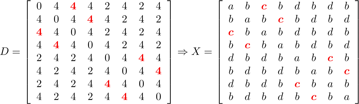
Upon some numerical investigation, we found the aforesaid assertion to be false. We found examples of subcodes of the first order binary Reed Muller code, for which identical entries in one row of $\Gamma$ resulted in distinct entries in the corresponding row of $X$ (see Fig. 1).

This breaking of symmetry from $\Gamma\to X$ led us to look into multiple orbits, and develop the mathematics to rigorously understand the optimal measurements for CGU sets, which encapsulate all linear codes. This in turn led us to generalize and simplify the previous results for GU sets as well, which are presented in Section IV. Our general results on MPE measurements for CGU sets are presented in Section V.

We say that a set of states is geometrically uniform (GU) if there is a group $G$ acting transitively on them i.e., for every two states $|\psi_{i}\rangle$ and $|\psi_{j}\rangle$ there exists a group element $g\in G$ such that $R(g)|\psi_{i}\rangle=|\psi_{j}\rangle$, where $R$ is some representation of the group $G$. This implies that all the elements of the set are obtained from a single element, say $|\psi_{1}\rangle$ by the action of the group. If the states are linearly independent, then the representation of the group on the space spanned by the states is the induced representation of the trivial representation of the stabilizer subgroup of $|\psi_{1}\rangle$. For a state discrimination problem to be GU, one usually assumes that the priors associated with the states in the GU set are the same for all states. The PGM was proved to be optimal for cyclic groups in [15], for abelian groups in [16] and for non-abelian groups in [19]. The pretty good measurement has been defined in [17] and [18] as a measurement to discriminate between the states $\rho_{i}$ with priors $p_{i}$. The measurement operators of the PGM are given by $\Pi_{i}=p_{i}\rho^{-1/2}\rho_{i}\rho^{-1/2}$, where $\rho=\sum_{i}p_{i}\rho_{i}$. If the states are pure ($\rho_{i}=|\psi_{i}\rangle\langle\psi_{i}|$) and linearly independent, this measurement becomes a projective measurement. Consider the polar decomposition of the matrix $M$ (defined in Eq. (3)). Observe that $\rho=MM^{\dagger}$ and so $U=\rho^{-1/2}M$. The columns of $U$ form the measurement basis of the PGM. From the left polar decomposition, notice that the columns of $U$ are also the measurement basis if the solution matrix $X$ coincides with $P=\sqrt{M^{\dagger}M}$. Since $P$ is Hermitian, it would be the solution of Eqs. 1 and 2 if, in addition, all the diagonal elements of $P$ are equal (since the priors are equal). To see that this is true for geometrically uniform states, observe that $\rho$ commutes with the representation $R$ and $x_{kk}=\langle w_{k}|\psi_{k}\rangle=\langle w_{1}|R(g)^{-1}R(g)|\psi_{1}\rangle=\langle w_{1}|\psi_{1}\rangle=x_{11}$.

Now we describe the measurement using non-abelian group representation theory along the lines of [15, 16] where it was done for abelian groups. In accordance with the action of the group, we have $|\psi_{i}\rangle=U(g_{i})|\psi_{1}\rangle$ for any $i$. We assume that the priors $p_{i}$ are all the same. Any transitive permutation action on a linearly independent set is an induced representation. We pick a base point, say $|\psi_{1}\rangle$ and with respect to this point, there is a subgroup $G_{0}$ of $G$ which stabilizes $|\psi_{1}\rangle$. The representation on the vector space spanned by $|\psi_{i}\rangle$ is the induced representation of the trivial representation of $G_{0}$ to $G$. If the set of states is $S$, then we have that $|S|=|G|/|G_{0}|$.

The Yuen, Kennedy, Lax conditions are

where $\psi_{i}=|\psi_{i}\rangle\langle\psi_{i}|$. Since the optimal measurement basis for a GU set is also GU, it is easy to see that we only need the equations where in the first two $i=1$.

Let the optimal measurement basis be given by $\{|w_{i}\rangle\}$ which are also GU under the $G$ action (and let $\Pi_{i}=|w_{i}\rangle\langle w_{i}|$). Therefore we have

Now let this representation consist of irreducible representations $\lambda$ with multiplicity $m_{\lambda}$. Consider the Fourier basis $|\lambda,m,k\rangle$ where $\lambda$ labels the irreducible representation, $m$ its multiplicity and $k$ its representation space whose dimension is denoted $d_{\lambda}$. The matrices $U(g)$ are block diagonal in this basis and therefore the operator $\Upsilon$ is also block diagonal by Schur’s lemma. In order to find the probability of error, we need to access to an arbitrary matrix element of $\Upsilon$ inside the blocks. Following Helstrom [15] (who worked this out for cyclic groups), we have

We denote $\psi_{1}$ and $\Pi_{1}$ as $\psi$ and $\Pi$ respectively. The action of any $U(g)$ on the state $|\lambda,m,k\rangle$ is given as follows

where $\lambda(g)_{k^{\prime},k}$ is the $k^{\prime},k$ matrix entry of the irreducible representation $\lambda$. Using this we get

Using the orthogonality relations among matrix entries of irreducible representations, we obtain

One can check that $\Upsilon$ is block diagonal with the blocks given by multiplicity spaces. Let $\phi=(1/|S|)\psi$. Now using the YKL equations, inside these invariant spaces, we see that

where $x_{\lambda,m,k}=\langle\lambda,m,k|\phi\rangle$ and $\gamma_{\lambda,m,k}=\langle\lambda,m,k|w\rangle$. In order to find the optimal measurement, we need to solve for $\gamma$. Suppose that $\gamma_{\lambda,m,k}=x_{\lambda,m,k}/c_{\lambda,m}$, where we need to solve for $c_{\lambda,m}$. We have from Eq. 8 that $\Upsilon_{\lambda,m}=c_{\lambda,m}\langle\phi|w\rangle$, if $\gamma_{\lambda,m,k}\neq 0$. We have that

Using the above two equations for $\Upsilon_{\lambda,m}$ we get that

The solution of the above equation is

We also need to check that $\Upsilon-\phi\geq 0$ for this solution. In order to do this, let $|\mu\rangle$ be an arbitrary normalized state. Then the above equation becomes $\langle\mu|(\Upsilon-\phi)|\mu\rangle\geq 0$. The left hand side can be written in the Fourier basis as

Now consider the second half of the above expression

where the last line was obtained through Cauchy-Schwartz. This shows that the $\gamma$ are the solutions. We can assume that the basis of the multiplicity space is picked in such a way that $x_{\lambda,m,k}$ is non-zero for only one $m$. Then $c_{\lambda,m}=\sqrt{\text{Tr}(P_{\lambda}\psi)/d_{\lambda}}$ and

where $P_{\lambda}$ is the projector onto the isotypic space $\lambda$.

We now calculate the probability of success using this expression. The probability of success is given by $P_{s}=|\langle w|\psi\rangle|^{2}$. This can be written as

For any group with a representation $U$, an expression for $P_{\lambda}$ is given by (for a character $\chi_{\lambda}$)

One can simplify the expression $\langle\psi|P_{\lambda}|\psi\rangle$ as follows.

But we have $\langle\psi|U(g)|\psi\rangle=\langle\psi|U(g_{1}gg_{2})|\psi\rangle$ for all $g_{1},g_{2}\in G_{0}$, where $G_{0}$ is the stabilizer group of $|\psi\rangle$ i.e., the subgroup of $G$ such that $U(g)|\psi\rangle=|\psi\rangle$, $\forall g\in G_{0}$. This means

where $i$ is a sum over $(G_{0},G_{0})$ double coset representatives and $C_{i}$ is the double coset. This sum can be further simplified to

where $g_{i}$ is the double coset representative of the double coset $C_{i}$. This can further be written as

where $\chi_{\lambda}(C_{i})=(1/|G_{0}|)\sum_{g\in C_{i}}\chi_{\lambda}(g^{-1})$. This gives an explicit formula for the probability of success. This means that if we can find the sum of the character values of the elements of a double coset easily, then we can obtain the formula for the probability of success. In the next subsection, we show how to do this for a specific case.

In this section, we describe how to obtain the optimal measurement for CGU state sets. We use the Helstrom description of the problem of finding the optimal measurement for pure states i.e., by viewing it as the solution of a set of simultaneous equations. However, as we pointed out earlier, one need not obtain a unique solution. With every obtained solution, we have to check the third condition to find the right one. We again resort to representation theory to simplify the equations and obtain far fewer equations (in many practical cases of interest). We begin by recalling the set of simultaneous equations which give the solution given above in Eqs. 1 and 2. $X^{\dagger}X=\Gamma,\quad x_{km}x^{\ast}_{mm}=x_{kk}x^{\ast}_{mk}$ where $\Gamma$ is the Gram matrix of the set of states. Since we have CGU symmetry in the problem, the Gram matrix is symmetric about a group $G$ and its representation $U(g)$. Suppose this representation decomposes into irreducible spaces $\lambda$ of dimension $d_{\lambda}$ with multiplicity $m_{\lambda}$ (as before). Then the Gram matrix is block diagonal in this basis with a block corresponding to each irreducible representation. Denote these blocks as $\Gamma^{\prime}_{\lambda}$. These blocks also have a special structure where they are identity in the representation space i.e., $\Gamma^{\prime}_{\lambda}=\Gamma_{\lambda}\otimes I_{d_{\lambda}}$. We note that the solution $X$ would have the same block diagonal decomposition since it commutes with the same representation of $G$. Then we have that inside an isotopic space $X_{\lambda}^{\dagger}X_{\lambda}=\Gamma_{\lambda}$. Notice that these matrices are of dimension $m_{\lambda}\times m_{\lambda}$. Therefore, if the multiplicity spaces are small, then this task is easy. Now, solving for such an $X_{\lambda}$ can be done only up to a unitary since for any solution $X_{\lambda}$, $U_{\lambda}X_{\lambda}$ is also a solution, where $U_{\lambda}$ is an arbitrary unitary operator. In order to find a solution, we need to use the set of equations in Eq. 2.

We have developed a new and compact interpretation—using group representation theory—of the minimum probability of error (MPE) measurement for distinguishing a set of geometrically uniform pure quantum states—states that form a single orbit under the group action, i.e., a transitive action. We also give a representation theoretic proof that the pretty good measurement, or equivalently the least squares measurement is the optimal (MPE) measurement for a GU set of states. More importantly, this representation theoretic framework gives explicit formulae for the minimum probability of error. This is useful in comparing the relative performance of various receivers. Using the same framework, we then extended our analysis to construct optimal measurements for compound geometrically uniform (CGU) state sets, which are states that form multiple orbits under the group action. CGU sets appear in many practical problems, particularly in transmitting classical data over a (quantum) optical channel. All linear codes formed using pure-state modulation constellations, which are known to achieve the quantum (Holevo) limit to the capacity of optical communication, are CGU sets. We showed how to compute the optimal measurement for CGU sets by reducing the problem to solving a few simultaneous equations. The number of equations depends on the sizes of the multiplicity spaces of irreducible representations. For many group representations (such as those of several practical good linear codes), this is a lot more tractable than solving large semi-definite programs, in order to solve—by brute force—the Yuen-Kennedy-Lax conditions [1] for determining optimal measurements for discriminating an arbitrary set of pure states with given pairwise inner products. We showed one example each of the evaluation of optimal measurements for GU and CGU states, respectively.

It is known that coherent-state (laser light) modulation is sufficient to achieve the Holevo capacity, the ultimate rate of reliable classical communication over a lossy-noisy optical channel [29, 30]. It is also known that linear codes (over an underlying coherent-state modulation) along with optimal measurements—which are CGU sets by definition—suffice to attain the Holevo capacity [28]. There is however a significant gap between the Holevo capacity and the Shannon capacity of the optical channel attainable by conventional optical receivers, viz., homodyne, heterodyne, and direct-detection receivers [31], and the gap widens in the low photon number regime [32]. It would be interesting to investigate explicit finite blocklength code families with good symmetry properties, whose rate performance along with the respective optimal measurements—calculated exactly by the general method we developed—bridges the aforesaid capacity gap. It would also be interesting to develop rigorous foundations for translating the optimal CGU measurement, to an algorithmic design of structured optical receivers built using a small universal set of known optical components and ancilla states, that can implement the optimal measurement on any given linear code. In the high photon number regime on the other hand, heterodyne detection is known to be asymptotically capacity optimal. However, in the high photon number regime, the improvement attained by the MPE measurement (over conventional optical receivers) in the error exponent in discriminating symbols of a modulation constellation (as seen in our GU and CGU examples in this paper, and also in Ref. [26]) translates to a superior finite blocklength rate achievable by the MPE measurement, even though heterodyne detection is capacity-optimal in this regime [33]. This suggests that translating our development in this paper to an algorithmic design of structured MPE-attaining optical receivers, may also have a benefit in the high photon number transmission regime, in terms of the finite-codelength rate performance.

We recall some basic facts of representation theory needed for the results in this paper and then show how to obtain the double coset sums in Eq. 16. Given any finite group $G$ and a complex vector space $V$, a linear map $\Phi:G\rightarrow\text{End}(V)$ which takes the group identity to the identity endomorphism is called a representation of $G$. Often, the space $V$ is called the representation. If there exists a subspace $W$ such that the map $\Phi$ is taken to the subspace for every element $G$, $W$ is called a sub-representation or an invariant subspace of $V$. The orthogonal complement of $W$ in $V$ will also be an invariant space. For any invariant space, the space itself and the trivial subspace consisting of the zero vector is always an invariant space. If the only invariant spaces of $V$ are the trivial space and itself, then $V$ is called an irreducible representation. Every finite group has a finite set of irreducible representations (sometimes called irreps) associated with it. Any representation can be decomposed into irreducible representations, where there may be many copies of a given irreducible representation in it. Invariant spaces of a group can be related to eigenspaes of an operator that is symmetric with respect to that group. More precisely, suppose that a matrix $A$ commutes with a representation of a group $G$ i.e., $U(g)A=AU(g)$ for all $g\in G$. Then the invariant spaces of $G$ lie inside eigenspaces of $A$. Suppose that $U$ has the following block diagonal decomposition

where $m_{\lambda}$ is the multiplicity space of the irrep $\lambda$ i.e., the number of times $\lambda$ appears in $U$. Then $A$ has the decomposition given by

where $A_{\lambda}$ is a matrix inside the multiplicity space and $d_{\lambda}$ is the dimension of $\lambda$. Note that if, in particular, $m_{\lambda}=1$, then $A_{\lambda}$ is one-dimensional and therefore is an eigenvalue of $A$. Even if $m_{\lambda}\neq 1$ but are small, we only need to diagonalize $A_{\lambda}$ for all $\lambda$ to determine the eigenvalues of $A$.

Now, we give the details of the calculations used to produce Eq. 16. The case for the trivial representation is simple. We explain here how to obtain the coset sums for the standard representation (denoted $b$) and the representation we denoted as $c$. We assume familiarity with the representation theory of the symmetric group. The double coset sum for $C_{0}$ is also trivial to obtain since $\chi_{x}(C_{0})$ (where $x$ represents $b$ or $c$) is the multiplicity of the trivial $G_{0}$ representation in $x$. This, by Frobenius reciprocity, is the multiplicity of the representation $x$ in the induced representation, which is $1$ for both $b$ and $c$. So, now if we evaluate the double coset sum $\chi_{x}(C_{1})$, then because both $b$ and $c$ are non-trivial irreducible representations, $\chi_{x}(C_{2})=-1-\chi_{x}(C_{1})$. Thus, we only need to evaluate one double coset sum $\chi_{x}(C_{1})$ for $b$ and $c$. In order to do this, note that the double coset sum is actually a multiple of a coset sum i.e., $\chi_{x}(C_{1})=2(N-2)\chi_{x}((13)G_{0})$. Now in order to evaluate $\chi_{x}((13)G_{0})$, find the trivial $G_{0}$ states in the induced representation. First, we represent the states in the induced representation as $|\{i,j\}\rangle$ (and there are ${N\choose 2}$ of these and they form an orthonormal basis of the induced representation). One can see that there are three trivial $G_{0}$ states (this follows from Frobenius reciprocity and the fact that this induced representation is multiplicity free). The first one is also a trivial $S_{N}$ state and is $\sum_{i,j:i\neq j}|\{i,j\}\rangle$ (denote this by $|t\rangle$). The second one comes from the standard $S_{N}$ representation (i.e., representation $b$). Note that the states in the representation $b$ are given by

Therefore, the (unnormalized) trivial $G_{0}$ state in $b$ can be seen to be $|s_{1}\rangle+|s_{2}\rangle$ (denote this by $|u\rangle$). Now, we can find $\chi_{b}(C_{1})$ as

This turns out to be $N-4$. Therefore, $\chi_{b}(C_{2})=-(N-3)$. Now, in $c$, the trivial $G_{0}$ state turns out to be (denoted $|v\rangle$).

The double coset sum $\chi_{c}(C_{1})$ can be calculated as follows.