Form factors of the isovector scalar current and the $\eta\pi$ scattering phase shifts

Let us introduce the following two form factors associated with the isospin one charged scalar operator $\bar{u}d$

	$\displaystyle B_{0}\,F_{S}^{\eta\pi}(s)={\langle\eta(p_{1})\pi^{+}(p_{2})|\bar{u}d(0)|0\rangle}$
	$\displaystyle B_{0}\,F_{S}^{K\bar{K}}(s)={\langle{\bar{K}^{0}}(p_{1}){K^{+}}(p_{2})|\bar{u}d(0)|0\rangle}$		(2)

where $s=(p_{1}+p_{2})^{2}$. We have computed these form factors at next-to-leading order (NLO) in the chiral expansion. The detailed expressions are given in appendix A. From eqs. (52), (53) in that appendix, it is easy to derive the expressions of the scalar radii, which are defined as

$${\langle r^{2}\rangle}_{S}^{PQ}=6{\dot{F}_{S}^{PQ}(0)}/{F_{S}^{PQ}(0)}\ .$$

(3)

For $\eta\pi$ and $K\bar{K}$ one obtains

		$\displaystyle{\langle r^{2}\rangle}_{S}^{\eta\pi}=\dfrac{6}{F_{\pi}^{2}}\Big[4\,L^{r}_{5}+\dfrac{1}{16\pi^{2}}\,\Big(-\dfrac{3}{4}L_{K}-\dfrac{11}{12}\Big)+\dfrac{m_{\pi}^{2}}{3}\,\bar{J}^{\prime}_{\pi\eta}(0)\Big]$		(4)
		$\displaystyle{\langle r^{2}\rangle}_{S}^{K\bar{K}}=\dfrac{6}{F_{\pi}^{2}}\Big[4\,L^{r}_{5}+\dfrac{1}{16\pi^{2}}\Big(-\dfrac{1}{2}\,L_{\eta}-\dfrac{1}{4}\,L_{K}-\dfrac{1}{2}\,R_{\pi\eta}-\dfrac{1}{4}\Big)\ -\dfrac{2m_{K}^{2}}{3}\,\bar{J}^{\prime}_{\pi\eta}(0)\Big]\ ,$		(5)

where $L_{P}$, $R_{PQ}$ are logarithmic functions of the pseudo-scalar meson masses,

$$L_{P}=\log\frac{m_{P}^{2}}{\mu^{2}},\quad R_{PQ}=\frac{m_{P}^{2}\log(m_{P}^{2}/m_{Q}^{2})}{m_{P}^{2}-m_{Q}^{2}}\ ,$$

(6)

with $\mu$ a renormalisation scale. These scalar radii depend on only one of the Gasser-Leutwyler coupling constants [23], $L^{r}_{5}$. It is instructive to compare them with the analogous $K\pi$ scalar radius associated with the strangeness changing scalar current, which also depends only on $L^{r}_{5}$ [24],

$${\langle r^{2}\rangle}_{S}^{K\pi}=\dfrac{6}{F_{\pi}^{2}}\Big[4\,L^{r}_{5}-\dfrac{1}{8}\dfrac{1}{16\pi^{2}}\Big(6L_{K}+5R_{\pi K}+R_{\eta K}\Big)\Big]+\delta_{2}$$

(7)

The explicit expression of $\delta_{2}$, from ref. [24], is reproduced in appendix A. One remarks that the three scalar radii ${\langle r^{2}\rangle}_{S}^{\eta\pi}$, ${\langle r^{2}\rangle}_{S}^{K\bar{K}}$, ${\langle r^{2}\rangle}_{S}^{K\pi}$ have exactly the same dependence on the coupling $L^{r}_{5}$, which means that they should be equal in the large $N_{c}$ limit of QCD. In reality, they are rather different. Using e.g. $L^{r}_{5}=(1.23\pm 0.06)\cdot 10^{-3}$ (from ref. [25], see sec. 2.3 below) one finds²² 2 The following input numerical values are used throughout this paper (all in GeV): $m_{\pi}=0.139568$, $m_{K}=0.4957$, $m_{\eta}=0.547853$, $F_{\pi}=0.09221$. for $\eta\pi$ and $K\bar{K}$

$$\begin{array}[]{ll}{\langle r^{2}\rangle}^{\eta\pi}_{S}=&0.092\pm 0.007\ \hbox{fm}^{2}\ ,\\ {\langle r^{2}\rangle}^{K\bar{K}}_{S}=&0.136\pm 0.007\ \hbox{fm}^{2}\ ,\\ \end{array}$$

(8)

while for $K\pi$, one finds,

$${\langle r^{2}\rangle}^{K\pi}_{S}=0.177\pm 0.007\ \hbox{fm}^{2}\ .$$

(9)

This shows that the $\eta\pi$ scalar radius is suppressed by a factor of two as compared to the $K\pi$ scalar radius.

We consider the three scattering amplitudes involving the $\eta\pi^{+}$ and the ${\bar{K}^{0}}{K^{+}}$ channels and we label the $\eta\pi^{+}$ channel as 1 and the ${\bar{K}^{0}}{K^{+}}$ channel as 2. At chiral order $p^{2}$ the amplitudes read,

$$\begin{array}[]{l@{}l}{\cal T}^{11}_{(2)}(s,t,u)=&\dfrac{m_{\pi}^{2}}{3F_{\pi}^{2}}\\[8.5359pt] {\cal T}^{12}_{(2)}(s,t,u)=&\dfrac{\sqrt{6}}{12F_{\pi}^{2}}\,(3s-4m_{K}^{2})\\[8.5359pt] {\cal T}^{22}_{(2)}(s,t,u)=&\dfrac{1}{4F_{\pi}^{2}}(s+(t-u))\ .\\ \end{array}$$

(10)

The corrections of chiral order $p^{4}$ to these amplitudes can be expressed in terms of a set of functions of one variable, analytic with a right-hand cut, according to the so-called reconstruction theorem [26] (see also the review [27]),

$$\begin{array}[]{ll}{\cal T}^{11}_{(4)}(s,t,u)&=U_{0}^{11}(s)+U_{0}^{11}(u)+W_{0}^{11}(t)\\[5.69046pt] {\cal T}^{12}_{(4)}(s,t,u)&=U_{0}^{12}(s)+\left[W_{0}^{12}(t)+(s-u)W_{1}(t)+(t\leftrightarrow u)\right]\\[5.69046pt] {\cal T}^{22}_{(4)}(s,t,u)&=U_{0}^{22}(s)+(t-u)U_{1}(s)+V_{0}(t)+(s-u)V_{1}(t)+W_{0}^{22}(u)\ .\\ \end{array}$$

(11)

The detailed expressions of the functions $U_{0}^{ab}$, $W_{0}^{ab}$, $U_{j}$, $V_{j}$ are given in appendix B. The resulting amplitudes are equivalent to previous calculations [1, 7]. We define the partial-wave amplitudes as

$$T_{J}^{ab}(s)=\frac{1}{32\pi}\int_{-1}^{1}{\cal T}^{ab}(s,t(z^{ab}),u(z^{ab}))\,dz^{ab}$$

(12)

such that the unitarity relation, in matrix form, reads

$${\rm Im\,}\bm{T}_{J}(s)=\bm{T}_{J}(s)\,\bm{\Sigma}(s)\,\bm{T}^{\dagger}_{J}(s)=\bm{T}_{J}^{\dagger}(s)\,\bm{\Sigma}(s)\,\bm{T}_{J}(s)$$

(13)

with

$$\bm{\Sigma}(s)=\begin{pmatrix}\sigma_{1}(s)\theta(s-(m_{\eta}+m_{\pi})^{2})&0\\ 0&\sigma_{2}(s)\theta(s-4m_{K}^{2})\\ \end{pmatrix},$$

(14)

and

$$\sigma_{1}(s)=\frac{\sqrt{\lambda_{\eta\pi}(s)}}{s},\quad\sigma_{2}(s)=\sqrt{\frac{s-4m_{K}^{2}}{s}},\quad\lambda_{\eta\pi}(s)=(s-(m_{\eta}-m_{\pi})^{2})(s-(m_{\eta}+m_{\pi})^{2})\ .$$

(15)

The relation between the partial wave $S$- and $T$-matrices then reads

$$\bm{S}_{J}(s)=1+2i\sqrt{\bm{\Sigma}(s)}\,\bm{T}_{J}(s)\,\sqrt{\bm{\Sigma}(s)}\ .$$

(16)

In eq. (12), $z^{ab}$ designate the cosines of the centre-of-mass scattering angles, which are related to the Mandelstam variables by

$$\begin{array}[]{l}t,u(z^{11})=\frac{1}{2}\left(2m_{\eta}^{2}+2m_{\pi}^{2}-s\pm\dfrac{\lambda_{\eta\pi}(s)z^{11}-\Delta_{\eta\pi}^{2}}{s}\right)\\[5.69046pt] t,u(z^{12})=\frac{1}{2}\left(m_{\eta}^{2}+m_{\pi}^{2}+2m_{K}^{2}-s\pm\sqrt{\lambda_{\eta\pi}(s)}\,\sigma_{2}(s)\,z^{12}\right)\\[5.69046pt] t,u(z^{22})=\frac{1}{2}(4m_{K}^{2}-s)(1\mp z^{22})\\ \end{array}$$

(17)

with $\Delta_{\eta\pi}=m_{\eta}^{2}-m_{\pi}^{2}$. The first two of these relations become singular when $s\to 0$. This implies that the chiral expansions of the $\eta\pi\to\eta\pi$ and $\eta\pi\to K\bar{K}$ partial-wave amplitudes become invalid when $s$ is too close to zero. If we assume a domain of validity for the expansion of the unprojected amplitudes when $|s|,\,|t|,\,|u|\mathrel{\raise 2.58334pt\hbox{$<$}\kern-7.7778pt\lower 2.79857pt\hbox{$\sim$}}0.5$ $\hbox{GeV}^{2}$, then the chiral expansions of the partial-wave amplitudes $T^{11}_{J}$, $T^{12}_{J}$ should converge with $s$ lying in the range $0.17\mathrel{\raise 2.58334pt\hbox{$<$}\kern-7.7778pt\lower 2.79857pt\hbox{$\sim$}}s\mathrel{\raise 2.58334pt\hbox{$<$}\kern-7.7778pt\lower 2.79857pt\hbox{$\sim$}}0.5$ $\hbox{GeV}^{2}$ and $0.05\mathrel{\raise 2.58334pt\hbox{$<$}\kern-7.7778pt\lower 2.79857pt\hbox{$\sim$}}s\mathrel{\raise 2.58334pt\hbox{$<$}\kern-7.7778pt\lower 2.79857pt\hbox{$\sim$}}0.5$ $\hbox{GeV}^{2}$ respectively.

From now on, we will consider only the $J=0$ partial-wave and will drop the $J$ subscript. With the subscript now indicating the chiral order, the $J=0$ partial-wave amplitudes at $O(p^{2})$ are simply derived from (10)

$$T^{11}_{(2)}(s)=\frac{1}{16\pi}\frac{m_{\pi}^{2}}{3F_{\pi}^{2}},\quad T^{12}_{(2)}(s)=\frac{1}{16\pi}\frac{\sqrt{6}(3\,s-4\,m_{K}^{2})}{12F_{\pi}^{2}},\quad T^{22}_{(2)}(s)=\frac{1}{16\pi}\frac{s}{4F_{\pi}^{2}}\ .$$

(18)

The corrections of chiral order $p^{4}$ to these $J=0$ partial-wave amplitudes can be written as

$$T^{ij}_{(4)}(s)=\dfrac{1}{16\pi}\left(U_{0}^{ij}(s)+\hat{U}_{0}^{ij}(s)\right)$$

(19)

where

		$\displaystyle\hat{U}_{0}^{11}(s)=\frac{1}{2}\int_{-1}^{1}dz^{11}\,\left(U_{0}^{11}(u)+W_{0}^{11}(t)\right)$
		$\displaystyle\hat{U}_{0}^{12}(s)=\int_{-1}^{1}dz^{12}\,\left(W_{0}^{12}(t)+(s-u)\,W_{1}(t)\right)$		(20)
		$\displaystyle\hat{U}_{0}^{22}(s)=\frac{1}{2}\int_{-1}^{1}dz^{22}\,\left(V_{0}(t)+(s-u)\,V_{1}(t)+W_{0}^{22}(u)\right)$

The functions $\hat{U}_{0}^{ij}(s)$ carry the left-hand cuts of the partial-wave amplitudes $T^{ij}$. These cuts are as follows [28]:

• $T^{11}$:

  A real cut on $[-\infty,(m_{\eta}-m_{\pi})^{2}]$ and a complex circular cut centred at $s=0$ with radius $\Delta_{\eta\pi}$.

• $T^{12}$:

  A real cut on $[-\infty,0]$ and a complex quasi-circular cut which intersects the real axis at $-\Delta_{\eta\pi}m_{K}/(m_{K}+m_{\eta})$ and $\Delta_{\eta\pi}m_{K}/(m_{K}+m_{\pi})$.

• $T^{22}$:

  A real cut on $[-\infty,4m_{K}^{2}-4m_{\pi}^{2}]$.

As a final remark, at NLO, each one of the functions $U_{0}^{ij}$, $W_{0}^{ij}$, $U_{1}$, $V_{j}$ can be written as the sum of a polynomial part and one involving a combination of functions $\bar{J}_{PQ}$ (see appendix B). The latter part is constrained by unitarity. For instance, for the functions $U_{0}^{ij}$, one can write, in matrix form,

$$\bm{U_{0}}(s)=\bm{P_{0}}(s)+(16\pi)^{2}\,\bm{T}_{(2)}(s)\begin{pmatrix}\bar{J}_{\pi\eta}(s)&0\\ 0&\bar{J}_{K\bar{K}}(s)\\ \end{pmatrix}\bm{T}_{(2)}(s)\ .$$

(21)

The values of the low-energy couplings (LEC’s) $L_{i}^{r}$, $i=1\cdots 8$ are needed in order to evaluate numerically the chiral amplitudes. A recent update of the values of the couplings $L_{i}^{r}$ has been presented in ref. [25] based on global fits involving a number of low energy observables. We reproduce in table 1 two sets of values which correspond to NLO expansions (which seem appropriate here since we are using NLO formulae). The set labelled (A) in table 1 corresponds to an unconstrained fit and it leads to rather large values of the couplings $L_{4}$, $L_{6}$ and $L_{2}-2L_{1}$ which are suppressed in the large $N_{c}$ limit [23]. The set (B) in the table corresponds to a fit which is constrained to enforce compatibility with the results from lattice QCD simulations on $L_{4}^{r}$ and $L_{6}^{r}$. We will consider it to be more plausible, since the strong deviations from the large $N_{c}$ limit are possibly an artifact of attempting to reproduce certain observables which are sensitive to NNLO rescattering effects (like the $I=J=0$ $\pi\pi$ scattering length) using NLO formulae. Fig. 1 illustrates the sensitivity of the $I=1$ amplitudes considered here to the $1/N_{c}$ suppressed couplings. The shape of the $\eta\pi\to\eta\pi$ amplitude is quite different if one uses the set (A) or the set (B). This is also reflected in the values of the $J=0$ threshold parameters. Defining the scattering length $a_{0}$ and the scattering range $b_{0}$ as in ref. [1],

$$\frac{2}{\sqrt{s}}\,T^{11}(s)=a_{0}+b_{0}\,p^{2}+\cdots$$

(22)

with $\sqrt{s}=\sqrt{m_{\pi}^{2}+p^{2}}+\sqrt{m_{\eta}^{2}+p^{2}}$, one finds

$$\begin{array}[]{lll}m_{\pi}\,a_{0}=6.7\cdot 10^{-3},&m_{\pi}\,b_{0}=-15.0\cdot 10^{-3}&(\hbox{Large }L_{4},\ L_{6})\\ m_{\pi}\,a_{0}=16.2\cdot 10^{-3},&m_{\pi}\,b_{0}=10.6\cdot 10^{-3}&(\hbox{Small }L_{4},\ L_{6})\ .\end{array}$$

(23)

The two sets of couplings thus lead to rather different values of the scattering length $a_{0}$ while the values of the scattering range $b_{0}$ differ in their sign. At leading chiral order, one has $m_{\pi}\,a_{0}=6.2\cdot 10^{-3}$, $b_{0}=0$. At NLO, a low-energy theorem (LET) for $a_{0}$ was derived in ref. [29], in the form of a linear relation

$$\left.a_{0}\right|_{NLO}=\lambda\,\left.a_{0,\pi\pi}^{2}\right|_{NLO}+\mu$$

(24)

where $a_{0,\pi\pi}^{2}$ is the $\pi\pi$ scattering length with $J=0$, $I=2$ and $\lambda$, $\mu$ are simple functions of the masses $m_{\pi}$, $m_{K}$, $m_{\eta}$ and the decay constants $F_{\pi}$, $F_{K}$. The most precise determinations of the $S$-wave $\pi\pi$ scattering lengths are based on Roy equations solutions. Using the values quoted in two recent analysis of these equations [14, 30] in the LET relation (24), one obtains

$$\begin{array}[]{lll}a_{0,\pi\pi}^{2}=-0.0444\pm 0.0010&(\hbox{ref.~\cite[cite]{[\@@bibref{Number}{Colangelo:2001df}{}{}]}})&\longrightarrow a_{0}=(-0.22\pm 6.26)\cdot 10^{-3}\\ a_{0,\pi\pi}^{2}=-0.042\pm 0.0040&(\hbox{ref.~\cite[cite]{[\@@bibref{Number}{GarciaMartin:2011cn}{}{}]}})&\longrightarrow a_{0}=(14.8\pm 25.0)\cdot 10^{-3}\ .\end{array}$$

(25)

This illustrates that the LET is practically useful only if $a_{0,\pi\pi}^{2}$ is known to a very high precision. The result of ref. [14] is associated with a rather small error of $2.5\%$. However, the result derived from the Roy equations concerns the physical value of the scattering length rather than the NLO value which enters into the LET. An additional error should therefore be introduced in eq. (25) in order to account for the difference $a_{0,\pi\pi}^{2}-\left.a_{0,\pi\pi}^{2}\right|_{NLO}$, which could easily be as large than $5\%$. This observation then limits the effectiveness of the LET for determining $a_{0}$.

The ${\bar{K}^{0}}{K^{+}}\to{\bar{K}^{0}}{K^{+}}$ partial-wave amplitude vanishes at $s=0$ at leading chiral order (18). This zero, however, is accidental since it is not associated with a soft pion theorem. Fig. 1 shows that, indeed, the NLO corrections are substantial. The corrections corresponding to the $L_{i}$ set (B), with small $1/N_{c}$ violations, have a more reasonable size than those from set (A). The amplitude $\eta\pi^{+}\to{\bar{K}^{0}}{K^{+}}$ has a zero at $s=4m_{K}^{2}/3$ at $O(p^{2})$ which corresponds to a soft pion Adler zero. Fig. 1 shows that the NLO corrections are rather small in this case and that there is little difference between the couplings of set (A) and set (B).

The crucial property of two-meson form factors is that they can be defined as analytic functions in the complex energy plane, with a cut lying on the positive real axis in the range $s>(m_{P}+m_{Q})^{2}$ [32]. In the asymptotic region, $|s|\to\infty$, the general arguments concerning exclusive processes in QCD [33] predict that a two-meson scalar form factor $F_{S}$ should obey a power law behaviour,

$$\left.F_{S}(s)\right|_{s\to\infty}\sim 1/s$$

(26)

up to logarithms. Making the assumption that the form factor $F_{S}$ has no zeros in the complex plane, one can derive a minimal phase dispersive representation (e.g. [34]),

$$F_{S}(s)=F_{S}(0)\,\exp\left[\frac{s}{\pi}\int_{s_{0}}^{\infty}\frac{\phi_{S}(s^{\prime})}{s^{\prime}\,(s^{\prime}-s)}\,\,ds^{\prime}\right]\ ,$$

(27)

where the phase is defined from $F(s+i\epsilon)=|F_{s}(s)|\exp(i\phi_{S}(s))$. The QCD asymptotic behaviour (26) is reproduced from eq. (27) provided that the phase has the asymptotic limit:

$$\lim_{s^{\prime}\to+\infty}\phi_{S}(s^{\prime})=\pi\ .$$

(28)

The scalar radius, finally, is given by a simple integral as a function of $\phi_{S}$,

$${\langle r^{2}\rangle}_{S}=\frac{6}{\pi}\int_{s_{0}}^{\infty}\frac{\phi_{S}(s^{\prime})}{(s^{\prime})^{2}}\,\,ds^{\prime}\ .$$

(29)

If $n$ complex zeros were present, then the right-hand side of eq. (27) would have to be multiplied by a polynomial of degree $n$ and the asymptotic phase would have to be $(n+1)\pi$. The minimality assumption is equivalent to stating that the increase of the phase in the energy region $\sqrt{s}>2$ GeV should be less than $\pi$. This is plausible since no sharp resonances are present in this region.

As emphasised in ref. [15], these phase relations are of particular interest for those form factors which involve at least one pion, $F_{S}^{\pi P}$ with $P=\pi$, $K$ or $\eta$ which interests us here. This is simply because the scattering amplitudes $\pi P\to\pi P$ are elastic in a finite low energy region. In this region, the form factor phase $\phi_{S}^{\pi P}$ is constrained from Watson’s theorem to be exactly equal to the elastic scattering phase shift. The energy region in which inelasticity can be neglected to a good approximation extends up to the $K\bar{K}$ threshold for $\pi\pi$ and we expect the same property to hold also³³ 3 The inelastic mode $\eta\pi\to 3\pi$ is allowed already at threshold but the $S$-wave projection vanishes by parity conservation (since $J^{P}=0^{-}$ for the $3\pi$ state). The modes $\eta\pi\to 5\pi$, $\eta\pi\to\eta 3\pi$ are strongly suppressed by phase space below one GeV. for $\pi\eta$. The asymptotic value of the form factor phase is also known and one may estimate that $\phi_{S}^{\pi P}$ should be smoothly approaching its asymptotic value when $\sqrt{s}\mathrel{\raise 2.58334pt\hbox{$>$}\kern-7.7778pt\lower 2.79857pt\hbox{$\sim$}}2$ GeV. There only remains to determine $\phi_{S}^{\pi P}$ in the intermediate energy region that is, in the case of $\eta\pi$, in the region $1\leq\sqrt{s}\mathrel{\raise 2.58334pt\hbox{$<$}\kern-7.7778pt\lower 2.79857pt\hbox{$\sim$}}2$ GeV. In this region, we further expect that the fastest energy variation should take place close to 1 GeV, associated with the sharp onset of inelasticity triggered by the presence of the $a_{0}(980)$ resonance which is known to couple strongly to the $K\bar{K}$ channel [35]. This suggests to consider a framework which takes into account only the dominant inelastic channel and ignores all the other ones. In this case, the two form factors $F_{S}^{\eta\pi}$, $F_{S}^{K\bar{K}}$ obey a closed set of Muskhelishvili-Omnès coupled integral equations,

$$\begin{pmatrix}F_{S}^{\eta\pi}(s)\\ F_{S}^{K\bar{K}}(s)\\ \end{pmatrix}=\dfrac{1}{\pi}\int_{(m_{\eta}+m_{\pi})^{2}}^{\infty}\dfrac{ds^{\prime}}{s^{\prime}-s}\begin{pmatrix}T^{11}(s)&T^{12}(s)\\ T^{12}(s)&T^{22}(s)\\ \end{pmatrix}^{*}\begin{pmatrix}\sigma_{1}(s^{\prime})\,F_{S}^{\eta\pi}(s^{\prime})\\ \sigma_{2}(s^{\prime})\,F_{S}^{K\bar{K}}(s^{\prime})\theta(s^{\prime}-4m_{K}^{2})\\ \end{pmatrix}\ .$$

(30)

These equations encode the property of analyticity of the form factors, the asymptotic behaviour (which allows for an unsubtracted dispersive representation) and two-channel unitarity. One can express the two-channel $S$-matrix in terms of two phase shifts and one inelasticity parameter in the usual way,

$$\bm{S}=\begin{pmatrix}\eta\,\hbox{e}^{2i\delta_{11}}&i\sqrt{1-\eta^{2}}\,\hbox{e}^{i(\delta_{11}+\delta_{22})}\\ i\sqrt{1-\eta^{2}}\,\hbox{e}^{i(\delta_{11}+\delta_{22})}&\eta\,\hbox{e}^{2i\delta_{22}}\\ \end{pmatrix},\quad 0\leq\eta\leq 1\ .$$

(31)

We assume the following asymptotic conditions on the $S$-matrix parameters

$$\lim_{s\to\infty}\eta(s)=1,\quad\lim_{s\to\infty}\delta_{11}(s)+\delta_{22}(s)=2\pi~,$$

(32)

which ensure that the so called Noether index [36] (see also [37]) associated with the set of singular integral equations (30) is equal to two. This, in general, implies that a unique solution is obtained once two arbitrary conditions are specified, for instance the values at $s=0$: $F_{S}^{\eta\pi}(0)$, $F_{S}^{K\bar{K}}(0)$, and that the solution form factors behave asymptotically as $1/s$ [37].

In summary, solving the set of eqs. (30) for the form factors $F_{S}^{\eta\pi}$, $F_{S}^{K\bar{K}}$, one obtains a phase $\phi_{S}^{\eta\pi}$ which correctly matches with both the low and high energy limits expectations and provides an interpolating model in the intermediate energy region. The phase $\phi_{S}^{K\bar{K}}$ is also provided. In this case, however, there is no constraint from Watson’s theorem at low energy. One expects that the form factor $F_{S}^{K\bar{K}}$ will be more sensitive than $F_{S}^{\eta\pi}$ to the influence of the neglected inelastic channels.

More generally, one can use the system of equations (30) to define the Omnès matrix $\Omega^{ij}(s)$ which generalises the usual Omnès function [38]. Such a generalisation was first discussed in the case of $\pi\pi-K\bar{K}$ scattering in refs. [39, 40]. The first column of the Omnès matrix is obtained by solving the system with the boundary conditions $\Omega^{11}(0)=1$, $\Omega^{21}(0)=0$ and the second column by solving with the conditions $\Omega^{12}(0)=0$, $\Omega^{22}(0)=1$ (see in ref. [13] an appropriate numerical method for solving the linear system). The Omnès matrix allows one to treat the final-state interaction problem taking into account inelastic rescattering. For instance, one can express the $I=1$ scalar form factors in terms of the $\bm{\Omega}$ matrix,

$$\begin{pmatrix}F_{S}^{\eta\pi}(s)\\ F_{S}^{K\bar{K}}(s)\\ \end{pmatrix}=\begin{pmatrix}\Omega^{11}(s)&\Omega^{12}(s)\\ \Omega^{21}(s)&\Omega^{22}(s)\\ \end{pmatrix}\begin{pmatrix}\,F_{S}^{\eta\pi}(0)\\ F_{S}^{K\bar{K}}(0)\\ \end{pmatrix}~.$$

(33)

Let us first consider the $\pi\eta\to\pi\eta$ amplitude below the $K\bar{K}$ threshold. In this region, $\eta\pi$ scattering should be approximately elastic. The $\pi\eta$ scattering phase shift below 1 GeV should be controlled by the values of the threshold parameters $a_{0}$, $b_{0}$ on the one hand and the properties of the $a_{0}(980)$ resonance on the other. We will consider that the values of $a_{0}$, $b_{0}$ corresponding to the set of $L_{i}^{\prime}s$ with small $L_{4}$, $L_{6}$ (set (B), see table 1) are the most plausible. In this case, $a_{0}$ and $b_{0}$ are both positive and one expects that the phase shift will be positive in the whole elastic region. A different possibility was investigated in ref. [49].

The $a_{0}(980)$ is a well established resonance but its shape is not well described by a simple Breit-Wigner form because of the vicinity of the $K\bar{K}$ threshold. This partly explains the dispersion in the values of the mass and width quoted by the PDG [50]: $m_{a_{0}}=980\pm 20$ MeV, $\Gamma_{a_{0}}=[50-100]$ MeV. A comparison of a number of determinations of the $T_{11}$ amplitude near the $K\bar{K}$ threshold based, in particular, on the popular Flatté model [51] is performed in ref. [52]. The corresponding $\eta\pi$ phase shifts are plotted on Fig. 10 of that reference, from which one can deduce that the value of the phase shift at the $K\bar{K}$ threshold lies around 90°,

$$\delta_{11}(2m_{K})=(90\pm 20)\degree\ .$$

(43)

This is also satisfied in the models of refs. [8] and  [9] which give, respectively, $\delta_{11}(2m_{K})=95\degree$ and $\delta_{11}(2m_{K})=77\degree$.

The $a_{0}(980)$ resonance corresponds to poles of the amplitude in the complex plane on the second and on the third Riemann sheets which can both be near the physical region since the mass is very close to the $K\bar{K}$ threshold. For definiteness, we will rely here on the recent determination by the KLOE collaboration [53]. It is based on measurements of the $\phi\to\eta\pi\gamma$ decay amplitude with both high precision and high statistics. Based on the best fit performed in ref. [53] (using the theoretical model from ref. [54]) the location of the poles can be deduced to be

$$\begin{array}[]{ll}\sqrt{s^{II}_{a_{0}(980)}}=&(994\pm 2-i\,(25.4\pm 5.0))\ \hbox{MeV}\\[7.11317pt] \sqrt{s^{III}_{a_{0}(980)}}=&(958\pm 13-i\,(60.8\pm 11.5))\ \hbox{MeV}\ .\\ \end{array}$$

(44)

In the $[1-2]$ GeV energy region, a second resonance, the $a_{0}(1450)$, first reported in ref. [55] was later identified in $\bar{p}p$ decays at rest (e.g. [56, 57, 58], see also [59] who re-analysed the data). This resonance should correspond to a pole on the third Riemann sheet. Based on the value of the mass and width quoted in the PDG, we can estimate

$$\sqrt{s_{a_{0}(1450)}^{III}}=(1474\pm 19-i\,(133\pm 7))\ \hbox{MeV}\ .$$

(45)

A further property of the $a_{0}(1450)$ is that it has approximately equal decay widths into $\pi\eta$ and into $K\bar{K}$. We will implement this feature by requiring that the $J=0$ cross sections for $\eta\pi\to\eta\pi$ and $\eta\pi\to K\bar{K}$ should be approximately equal when $\sqrt{s}=1.474$ GeV. In our two-channel framework, these cross sections have the following expressions in terms of the phase shifts and the inelasticity parameter

$$\sigma(\eta\pi\to\eta\pi)=\frac{\pi}{p_{\eta\pi}^{2}}\left|\eta\,\hbox{e}^{2i\delta_{11}}-1\right|^{2},\quad\sigma(\eta\pi\to K\bar{K})=\frac{\pi}{p_{\eta\pi}^{2}}\left(1-\eta^{2}\right)$$

(46)

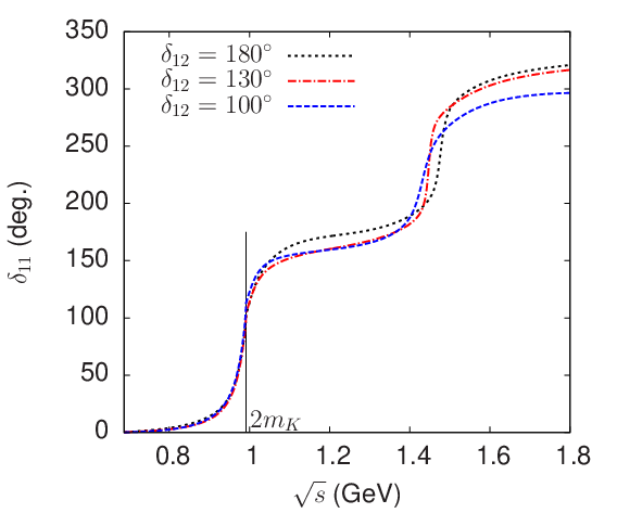
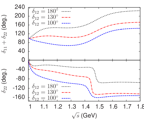
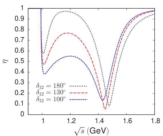
and we expect that $\eta$ should reach a minimum at the mass of the $a_{0}(1450)$ resonance. If the minimum is close to zero, the two cross sections will be approximately equal⁴⁴ 4 Equality of the two cross sections occurs either when $\eta=0$ or $\eta=\cos 2\delta_{11}$. In this situation, we expect a rapid variation of the phase shifts $\delta_{11}$, $\delta_{22}$ (possibly becoming discontinuous if $\eta=0$) at the energy $\sqrt{s}=m_{a_{0}(1450)}$. In contrast, the sum of the two phase shifts (which is also the phase of $S_{12}$) should be a smoothly varying function. It is convenient to characterise the global behaviour of the $S$-matrix in the $[1-2]$ GeV region in terms of the value of this phase sum $\delta_{11}+\delta_{12}$ when $\sqrt{s}=m_{a_{0}(1450)}$

$$\delta_{12}\equiv\left.\delta_{11}(\sqrt{s})+\delta_{22}(\sqrt{s})\right|_{\sqrt{s}=m_{a_{0}(1450)}}\ .$$

(47)

References

- [1] V. Bernard, N. Kaiser, U.G. Meißner, Phys.Rev. D44, 3698 (1991)
- [2] J. Kambor, C. Wiesendanger, D. Wyler, Nucl.Phys. B465, 215 (1996), hep-ph/9509374
- [3] A. Anisovich, H. Leutwyler, Phys.Lett. B375, 335 (1996), hep-ph/9601237
- [4] N. Achasov, S. Devyanin, G. Shestakov, Phys.Lett. B88, 367 (1979)
- [5] A.M. Abdel-Rehim, D. Black, A.H. Fariborz, J. Schechter, Phys.Rev. D67, 054001 (2003), hep-ph/0210431
- [6] J. Oller, E. Oset, J. Peláez, Phys.Rev. D59, 074001 (1999), hep-ph/9804209
- [7] A. Gómez Nicola, J. Peláez, Phys.Rev. D65, 054009 (2002), hep-ph/0109056
- [8] D. Black, A.H. Fariborz, J. Schechter, Phys.Rev. D61, 074030 (2000), hep-ph/9910351
- [9] A. Furman, L. Leśniak, Phys.Lett. B538, 266 (2002), hep-ph/0203255
- [10] J.F. Donoghue, J. Gasser, H. Leutwyler, Nucl.Phys. B343, 341 (1990)
- [11] J. Gasser, H. Leutwyler, Phys.Lett. B125, 325 (1983)
- [12] J. Gasser, U.G. Meißner, Nucl.Phys. B357, 90 (1991)
- [13] B. Moussallam, Eur.Phys.J. C14, 111 (2000), hep-ph/9909292
- [14] G. Colangelo, J. Gasser, H. Leutwyler, Nucl.Phys. B603, 125 (2001), hep-ph/0103088
- [15] F. Ynduráin, Phys.Lett. B612, 245 (2005), hep-ph/0501104
- [16] J.A. Oller, L. Roca, Phys.Lett. B651, 139 (2007), 0704.0039
- [17] S. Aoki et al. (JLQCD, TWQCD), Phys.Rev. D80, 034508 (2009), 0905.2465
- [18] V. Gülpers, G. von Hippel, H. Wittig, Phys.Rev. D89, 094503 (2014), 1309.2104
- [19] S. Aoki, Y. Aoki, C. Bernard, T. Blum, G. Colangelo et al. (FLAG Working Group) (2013), 1310.8555
- [20] M. Jamin, J.A. Oller, A. Pich, Nucl. Phys. B622, 279 (2002), hep-ph/0110193
- [21] J.M. Flynn, J. Nieves, Phys.Rev. D75, 074024 (2007), hep-ph/0703047
- [22] B. El-Bennich, A. Furman, R. Kamiński, L. Leśniak, B. Loiseau et al., Phys.Rev. D79, 094005 (2009), 0902.3645
- [23] J. Gasser, H. Leutwyler, Nucl.Phys. B250, 465 (1985)
- [24] J. Gasser, H. Leutwyler, Nucl.Phys. B250, 517 (1985)
- [25] J. Bijnens, G. Ecker (2014), 1405.6488
- [26] J. Stern, H. Sazdjian, N. Fuchs, Phys.Rev. D47, 3814 (1993), hep-ph/9301244
- [27] M. Zdrahal, J. Novotny, Phys.Rev. D78, 116016 (2008), 0806.4529
- [28] J. Kennedy, T.D. Spearman, Phys.Rev. 126, 1596 (1961)
- [29] B. Kubis, S.P. Schneider, Eur.Phys.J. C62, 511 (2009), 0904.1320
- [30] R. García-Martín, R. Kamiński, J. Peláez, J. Ruiz de Elvira, F. Ynduráin, Phys.Rev. D83, 074004 (2011), 1102.2183
- [31] Z.H. Guo, J. Oller, J. Ruiz de Elvira, Phys.Rev. D86, 054006 (2012), 1206.4163
- [32] G. Barton, Introduction to dispersion techniques in field theory, Lecture notes and supplements in physics (W.A. Benjamin, New York, 1965)
- [33] G.P. Lepage, S.J. Brodsky, Phys.Rev. D22, 2157 (1980)
- [34] M. Gourdin, Phys.Rept. 11, 29 (1974)
- [35] A. Astier, L. Montanet, M. Baubillier, J. Duboc, Phys.Lett. B25, 294 (1967)
- [36] F. Noether, Math. Ann. 82, 42 (1921)
- [37] N.L. Muskhelishvili, Singular Integral Equations (P. Noordhof, Groningen, 1953)
- [38] R. Omnès, Nuovo Cim. 8, 316 (1958)
- [39] O. Babelon, J.L. Basdevant, D. Caillerie, G. Mennessier, Nucl.Phys. B113, 445 (1976)
- [40] O. Babelon, J. Basdevant, D. Caillerie, M. Gourdin, G. Mennessier, Nucl.Phys. B114, 252 (1976)
- [41] M. Jamin, J.A. Oller, A. Pich, Nucl.Phys. B587, 331 (2000), hep-ph/0006045
- [42] A. Dobado, M.J. Herrero, T.N. Truong, Phys.Lett. B235, 134 (1990)
- [43] A. Dobado, J. Peláez, Phys.Rev. D47, 4883 (1993), hep-ph/9301276
- [44] J. Oller, E. Oset, Nucl.Phys. A620, 438 (1997), hep-ph/9702314
- [45] J. Oller, E. Oset, J. Peláez, Phys.Rev.Lett. 80, 3452 (1998), hep-ph/9803242
- [46] J. Oller, E. Oset, A. Ramos, Prog.Part.Nucl.Phys. 45, 157 (2000), hep-ph/0002193
- [47] F. Guerrero, J.A. Oller, Nucl.Phys. B537, 459 (1999), hep-ph/9805334
- [48] G. Ecker, J. Gasser, A. Pich, E. de Rafael, Nucl.Phys. B321, 311 (1989)
- [49] N. Achasov, G. Shestakov, Phys.Rev. D81, 094029 (2010), 1003.5054
- [50] K. Olive et al. (Particle Data Group), Chin.Phys. C38, 090001 (2014)
- [51] S.M. Flatté, Phys.Lett. B63, 224 (1976)
- [52] V. Baru, J. Haidenbauer, C. Hanhart, A.E. Kudryavtsev, U.G. Meißner, Eur.Phys.J. A23, 523 (2005), nucl-th/0410099
- [53] F. Ambrosino et al. (KLOE Collaboration), Phys.Lett. B681, 5 (2009), 0904.2539
- [54] G. Isidori, L. Maiani, M. Nicolaci, S. Pacetti, JHEP 0605, 049 (2006), hep-ph/0603241
- [55] M. Boutemeur, M. Poulet (GAMS), A new scalar meson decaying into and results of analysis at 100-Gev/c, in HADRON 89 (Editions Frontières, 1989)
- [56] C. Amsler et al. (Crystal Barrel Collaboration.), Phys.Lett. B333, 277 (1994)
- [57] A. Abele, S. Bischoff, P. Blum, N. Djaoshvili, D. Engelhardt et al., Phys.Rev. D57, 3860 (1998)
- [58] A. Bertin et al. (OBELIX Collaboration), Phys.Lett. B434, 180 (1998)
- [59] D. Bugg, Phys.Rev. D78, 074023 (2008), 0808.2706
- [60] A. Furman, L. Leśniak, Nucl.Phys.Proc.Suppl. 121, 127 (2003), hep-ph/0209304
- [61] B. Ananthanarayan, I. Caprini, G. Colangelo, J. Gasser, H. Leutwyler, Phys.Lett. B602, 218 (2004), hep-ph/0409222
- [62] H. Neufeld, H. Rupertsberger, Z.Phys. C68, 91 (1995)