Windowed Green Function method
for layered-media scattering

The solution of problems of scattering by obstacles or defects in presence of planar layered dielectric or conducting media has typically required use of Sommerfeld integrals and associated layer Green functions—which automatically enforce the relevant transmission conditions on the unbounded flat surfaces and thus reduce the scattering problems to integral equations on the obstacles and/or defects. As is well known, however, the numerical evaluation of layer Green functions and their derivatives, which amounts to computation of certain challenging Fourier integrals [8, 20], are extremely expensive and give rise to a significant bottleneck in layer-media simulations (see e.g. [6] for details). This paper presents a novel integral-equation approach for problems involving layered media. The new approach, which is based on use of certain “windowing” functions and considerations associated with the method of stationary phase, does not require use of expensive Sommerfeld integrals. Numerical experiments demonstrate that both the near- and far-field errors resulting from the proposed approach decrease faster than any negative power of the window size.

A variety of methods have been provided for the solution of problems of scattering by obstacles in presence of layered media. Amongst the most effective such approaches we mention 1) Methods which evaluate Sommerfeld integrals on the basis of path-integration in the complex plane [17, 7, 6, 18] (such approaches require numerical evaluation of integrals of functions that oscillate, grow exponentially in a bounded section of the integration path and, depending on the relative position of the source and observation points to the interface between the two media, may decay slowly at infinity); 2) The complex images method reviewed in [1] (a discussion indicating certain instabilities and inefficiencies in this method is presented in [7, section 5.5]); and 3) The steepest descent method [9, 10] which, provided the steepest descent path is known, reduces the Sommerfeld integral to an integral of an exponentially decaying function (unfortunately, however, the determination of steepest descent paths for each observation point can be challenging and expensive). As is well known, in any case, all of these methods entail significant computational costs [6].

The approach proposed in this paper bears similarities with certain “finite-section” methods in the field of rough-surface scattering. These methods utilize approximations based on truncated portions of a given unbounded rough surface [14, 22, 19] and, in some cases, they incorporate a “taper” [22, 21, 15] to eliminate artificial reflections from the edges of the finite sections. In fact the smooth taper function utilized in [15] (Figure 2 in that reference) resembles the smooth windowing function we use (Figure 2 below and reference [3]). But as indicated in comments provided in section 2 below in regards to certain slow-rise windowing functions, essential differences exist between the finite-section approaches and the methods proposed in this paper. In particular, with exception of the slow-rise windowing function method [3, 16], none of the previous tapered rough surface algorithms has demonstrated high-order convergence as the width of the finite sections tend to infinity.

In section 4 the proposed WGF method is compared against the high-order integral equation method recently introduced in [18], which is based on the accurate and efficient evaluation of the Sommerfeld integrals. In the examples considered in that section the proposed method is up to thousands of times faster, for a given accuracy, than a corresponding method based on the layer-Green-function. A much larger improvement in the computational cost is expected for problems of electromagnetic scattering by defects and obstacles in multi-layer structures in two- and three-dimensional spaces, which will be addressed in future contributions.

The proposed methodology is presented in sections 2 and 3. A variety of numerical results presented in sections 2 and 4 demonstrate the accuracy and speed of the proposed approach.

We consider two-dimensional TE and TM polarized dielectric transmission problems. As is well known, the $z$ components $u=E_{z}$ and $u=H_{z}$ of the total electric and magnetic fields satisfy the Helmholtz equation $\Delta u+k_{j}^{2}u=0$ in $\Omega_{j}$, $j=1,2$ (see Figure 1), where, letting $\omega>0$, $\varepsilon_{j}>0$, $\mu_{0}>0$, and $\sigma_{j}\geq 0$ denote the angular frequency, the electric permittivity, the magnetic permeability of vacuum, and the electrical conductivity, the wavenumber $k_{j}$ is defined by $k_{j}^{2}=\omega^{2}(\varepsilon_{j}+i\sigma_{j}/\omega)\mu_{0}$, $j=1,2$. In either case the total field is given by

$$u=\left\{\begin{array}[]{ccc}u_{1}+u^{\mathrm{inc}}&\mbox{in}&\Omega_{1},\\ u_{2}&\mbox{in}&\Omega_{2},\end{array}\right.$$

(1)

where denoting by $\alpha\in(-\pi,0)$ the incidence angle measured from the horizontal (see Figure 1), $u^{\mathrm{inc}}(\boldsymbol{x})=\operatorname{e}^{ik_{1}(x_{1}\cos\alpha+x_{2}\sin\alpha)}$, $u_{1}$ and $u_{2}$ denote the incident plane-wave and the reflected and transmitted waves, respectively. As is known (see e.g. [11]), the scattered and transmitted fields $u_{1}$ and $u_{2}$ admit the representations

	$\displaystyle u_{1}$	$\displaystyle=$	$\displaystyle\mathcal{D}_{1}\left[\varphi\right]-\mathcal{S}_{1}\left[\psi\right]\quad\mbox{ in }\quad\Omega_{1},$		(2a)
	$\displaystyle u_{2}$	$\displaystyle=$	$\displaystyle-\mathcal{D}_{2}\left[\varphi\right]+\mathcal{S}_{2}\left[\psi\right]\quad\mbox{ in }\quad\Omega_{2},$		(2b)

in terms of the total field $\varphi=u|_{\Gamma}$ and its normal derivative $\psi=\frac{\partial u}{\partial n}$ on $\Gamma$, where letting $G_{j}(\boldsymbol{x},\boldsymbol{y})=iH_{0}^{(1)}(k_{j}|\boldsymbol{x}-\boldsymbol{y}|)/4$, $j=1,2$ denote the free-space Green function for the Helmholtz equation with wavenumber $k_{j}$, the single- and double-layer potentials in equation (2) are defined by

$$\begin{split}\mathcal{S}_{j}[\eta](\boldsymbol{x})&=\int_{\Gamma}G_{j}(\boldsymbol{x},\boldsymbol{y})\eta(\boldsymbol{y})\,\text{d}s_{\boldsymbol{y}},\quad\mbox{and}\\ \mathcal{D}_{j}[\eta](\boldsymbol{x})&=\int_{\Gamma}\frac{\partial G_{j}}{\partial n_{\boldsymbol{y}}}(\boldsymbol{x},\boldsymbol{y})\eta(\boldsymbol{y})\,\text{d}s_{\boldsymbol{y}},\end{split}$$

(3)

respectively. By evaluating the fields (2) and their normal derivatives on $\Gamma$ and using the transmission conditions

$$u_{2}-u_{1}=u^{\mathrm{inc}},\quad\nu\frac{\partial u_{2}}{\partial n}-\frac{\partial u_{1}}{\partial n}=\frac{\partial u^{\mathrm{inc}}}{\partial n}\mbox{ on }\Gamma,$$

(with $\nu=1$ and $\nu=\varepsilon_{1}/\varepsilon_{2}$ in TE- and TM-polarizations respectively) we obtain the second-kind system of integral equations [12]

$$E\phi+T\phi=\phi^{\mathrm{inc}}\quad\mbox{on}\quad\Gamma$$

(4)

for the surface currents $\phi$, where

$$E=\left[\begin{array}[]{cc}1&0\\ 0&\frac{1+\nu}{2}\end{array}\right],\quad\phi=\left[\begin{array}[]{cc}u|_{\Gamma}\\ \frac{\partial u}{\partial n}|_{\Gamma}\end{array}\right],\quad\phi^{\mathrm{inc}}=\left[\begin{array}[]{cc}u^{\mathrm{inc}}|_{\Gamma}\\ \frac{\partial u^{\mathrm{inc}}}{\partial n}|_{\Gamma}\end{array}\right],$$

and where

$$T=\left[\begin{array}[]{cc}D_{2}-D_{1}&-\nu S_{2}+S_{1}\\ N_{2}-N_{1}&-\nu K_{2}+K_{1}\\ \end{array}\right]$$

(5)

is defined in terms of the boundary integral operators defined by the expressions $S_{j}[\eta](\boldsymbol{x})$ and $D_{j}[\eta](\boldsymbol{x})$ as well as

$$N_{j}[\eta](\boldsymbol{x})=\frac{\partial\mathcal{D}_{j}\eta}{\partial n}(\boldsymbol{x})\quad\mbox{and}\quad K_{j}[\eta](\boldsymbol{x})=\displaystyle\int_{\Gamma}\frac{\partial G_{j}}{\partial n_{\boldsymbol{x}}}(\boldsymbol{x},\boldsymbol{y})\eta(\boldsymbol{y})\,\text{d}s_{\boldsymbol{y}}$$

for $\boldsymbol{x}\in\Gamma$ and for $j=1$, 2.

Instead of solving the problem on the entire infinite plane a locally windowed problem could be used in an attempt to obtain local currents over relevant portions of the geometry. To pursue this idea we introduce a smooth windowing function $w_{A}$ (which is depicted in Figure 2) which is non-zero in an interval of length $2A$, and which has a slow rise: $w_{A}(x_{1})=f(x_{1}/A)$ for some fixed window function $f$. (Note that, with such a definition, $w_{A}$ rises from zero to one in a region of length proportional to $A$; see [3, 16]. As demonstrated in those references, the slow rise of the window function is essential to ensure fast convergence of the approximation.) For notational simplicity, the subindex $A$ will be dropped in what follows, and we will thus write $w(x_{1})$ instead of $w_{A}(x_{1})$. The parts of the boundary $\Gamma$ where $w(x_{1})\neq 0$ and $\widetilde{w}(x_{1})=1-w(x_{1})\neq 0$, further, will be denoted by $\Gamma_{A}$ and $\widetilde{\Gamma}_{A}$, respectively. The width $2A>0$ of the support of the window function $w$ is selected in such a way that $\widetilde{w}(x_{1})$ vanishes on any corrugations that exist on the surface $\Gamma$, as well as on any additional obstacles that may exist above and/or below $\Gamma$. (For notational simplicity our derivations are presented for cases for which the corrugations on the surface $\Gamma$ are the only departures from planarity, but, as demonstrated by Figure 12, our algorithms are also applicable in cases in which additional scatterers exist.)

Utilizing the windowing function $w$ and letting $W=w\cdot I$, where $I$ is the $2\times 2$ identity matrix, we consider the preliminary approximate equation

$$E\phi^{\star}+TW\phi^{\star}=\phi^{\mathrm{inc}}\quad\mbox{on}\quad\Gamma_{A}$$

(6)

(where the new unknown $\phi^{\star}$ is defined on $\Gamma_{A}$), and, in order to assess the errors inherent in this approximation, the form

$$E\phi+TW\phi=\phi^{\mathrm{inc}}-T(I-W)\phi\quad\mbox{on}\quad\Gamma_{A}$$

(7)

of the exact equation (4). Using integration-by-parts and employing the method of stationary-phase, it follows [5] that the term $T(I-W)\phi$ is super-algebraically small (i.e., smaller than $C_{p}(kA)^{-p}$ for any positive integer $p$ as $kA\to\infty$, where $C_{p}$ is a $p$-dependent constant) in the region $\{w=1\}$, and, thus, as shown in [5], that the solution $\phi^{\star}$ of (6) is a highly accurate approximation of $\phi$ throughout the center region $\{w=1\}$ of the surface $\Gamma_{A}$ provided $A$ is large enough. However, it is easy to see that, to correctly take into account fields reflected from the planar portions of the surface, the needed window sizes may be very large—especially so for incidence angles approaching grazing.

To demonstrate this fact we use equation (6) to approximate the solution of the TE problem of scattering of a plane-wave by a semi-circular bump of radius $a=1$ placed directly on top of a planar dielectric surface. The problem was discretized using a graded mesh over the surface of the bump and on the windowed portion of the planar interface, on the basis of a direct generalization of the Nyström method presented in [13] with $p=3$. For this example the wavenumbers $k_{1}$ and $k_{2}$ in the regions above and below the plane were set to $4\pi$ and $8\pi$, respectively, and approximately 20 points per unit length of the surface of the bump and the surrounding were used.

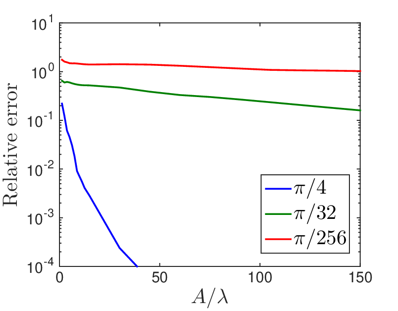
As shown in Figure 3, the naive windowing approach embodied in (6) requires large regions of the planar interface to be discretized as the incidence angle decreases. For accurate calculations at even moderate angles, a large number of wavelengths must be present in the window region, well beyond the extent of the non-planar local geometry.

In order to provide an insight into the source of the errors displayed in Figure 3 we present Figure 4. Figure 4(a) presents rays incident on the left planar region as well as their reflection and transmission. Clearly, in view of the incidence angle considered these reflected fields subsequently illuminate the defect. The blue rays, for example, represent the reflections that are correctly taken into account in the solution of equation (6) (since they lie within the windowed region), while the red arrows represent reflections that are neglected. Figure 4(b), on the other hand, represents reflections by the defect. The color-code in the left figure carries over to the right figure: the blue (resp. red) rays in Figure 4(b) represent the fields scattered by the defect which arise from the blue (resp. red) arrows in Figure 4(a). We remark that the scattering of the field represented by the red arrows is not taken into account by (6), which gives rise to the errors observed in Figure 3. We also note that the relatively fast convergence demonstrated by the blue curves in Figure 3 is explained by the fact that for near normal incidence ($\alpha\approx-\pi/2$) there is not much “red field” interacting with the defect. In contrast, for incidence near grazing ($\alpha\approx 0$), “red fields” from regions far away from the windowed area do interact with the defect. This explains the poor convergence properties demonstrated by the green and red curves in Figure 3: the fields neglected in the naive approach give rise to important contributions as $\alpha$ decreases.

To address this difficulty we consider again the exact integral equation (7) and we substitute the unknown density $\phi$ on the right-hand side of this equation by the corresponding (known) density $\phi^{f}$ associated with the problems of scattering and transmission of a plane-wave by a perfectly flat infinite plane. Since a superalgebraically small portion of the field reflected by the windowed region reflects back into the windowed region upon reflection from the plane outside the windowed region, we conclude that the error arising from the substitution of $\phi$ by $\phi^{f}$ results in superalgebraically small errors in equation (7) throughout the region $\{w=1\}$. We thus obtain the approximate equation

$$E\phi^{w}+TW\phi^{w}=\phi^{\mathrm{inc}}-T(I-W)\phi^{f}\quad\mbox{on}\quad\Gamma_{A},$$

(8)

whose solution $\phi^{w}$ is a superalgebraically close approximation of the exact solution $\phi$ throughout the region $\{w=1\}$. In order to evaluate the term $T(I-W)\phi^{f}$ we note that since $(I-W)\phi^{f}$ is zero everywhere $\Gamma_{A}$ deviates from the planar boundary $\Pi=\{(x_{1},x_{2})\in\mathbb{R}^{2}:x_{2}=0\}$ (depicted in Figure 1), we have

$$T(I-W)\phi^{f}=T_{\Pi}(I-W)\phi^{f},$$

where letting the layer potentials $\mathcal{S}^{\Pi}_{j}$ and $\mathcal{D}_{j}^{\Pi}$ be given by

$$\begin{split}\mathcal{S}^{\Pi}_{j}[\eta](\boldsymbol{x})&=\int_{\Pi}G_{j}(\boldsymbol{x},\boldsymbol{y})\eta(\boldsymbol{y})\,\text{d}s_{\boldsymbol{y}},\quad\mbox{and}\\ \mathcal{D}^{\Pi}_{j}[\eta](\boldsymbol{x})&=\int_{\Pi}\frac{\partial G_{j}}{\partial n_{\boldsymbol{y}}}(\boldsymbol{x},\boldsymbol{y})\eta(\boldsymbol{y})\,\text{d}s_{\boldsymbol{y}},\end{split}$$

(9)

the operator $T_{\Pi}$ is defined as

$$T_{\Pi}=\left[\begin{array}[]{cc}D^{\Pi}_{2}-D^{\Pi}_{1}&-\nu S^{\Pi}_{2}+S^{\Pi}_{1}\\ N^{\Pi}_{2}-N^{\Pi}_{1}&-\nu K^{\Pi}_{2}+K^{\Pi}_{1}\\ \end{array}\right]$$

in terms of the boundary integral operators defined by the expressions $S^{\Pi}_{j}[\eta](\boldsymbol{x})$ and $D^{\Pi}_{j}[\eta](\boldsymbol{x})$ as well as

$$N^{\Pi}_{j}[\eta](\boldsymbol{x})=\frac{\partial\mathcal{D}^{\Pi}_{j}\eta}{\partial n}(\boldsymbol{x})\big|_{\Gamma}\quad\mbox{and}\quad K^{\Pi}_{j}[\eta](\boldsymbol{x})=\displaystyle\int_{\Pi}\frac{\partial G_{j}}{\partial n_{\boldsymbol{x}}}(\boldsymbol{x},\boldsymbol{y})\eta(\boldsymbol{y})\,\text{d}s_{\boldsymbol{y}}$$

for $\boldsymbol{x}\in\Gamma$ and for $j=1$, 2. Thus equation (8) becomes

$$E\phi^{w}+TW\phi^{w}=\phi^{\mathrm{inc}}-T_{\Pi}\phi^{f}+T_{\Pi}W\phi^{f}\quad\mbox{on}\quad\Gamma_{A}.$$

(10)

Clearly the expression $T_{\Pi}W\phi^{f}$ can be evaluated by means of integration on the bounded region $\Pi\cap\{(x_{1},x_{2})\in\mathbb{R}^{2}:w(x_{1})\neq 0\}$, and the expression $T_{\Pi}\phi^{f}$ can be computed in closed form:

$$T_{\Pi}\phi^{f}=\left\{\begin{array}[]{ccl}\displaystyle\left[u^{\mathrm{inc}}-u^{f},\frac{\partial(u^{\mathrm{inc}}-u^{f})}{\partial n}\right]^{T}&\mbox{on}&\Gamma\setminus\Pi,\\ \displaystyle\left[u^{\mathrm{inc}}-u^{f},\frac{\partial(u^{\mathrm{inc}}-(1+\nu)u^{f}/2)}{\partial n}\right]^{T}&\mbox{on}&\Gamma\cap\Pi,\end{array}\right.$$

(11)

where $u^{f}$ is the total field resulting from the solution of the problem of scattering by the flat dielectric plane with boundary $\Pi$ [8, Chapter 2].

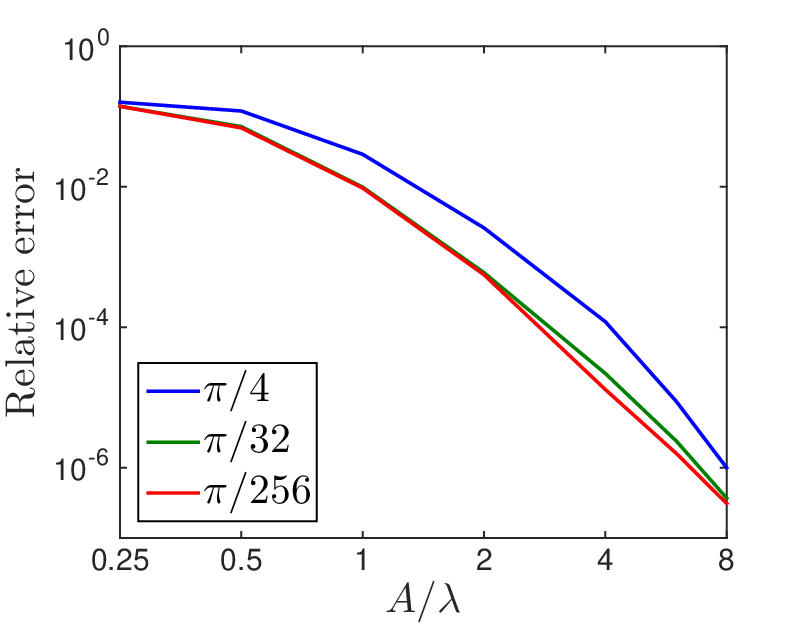
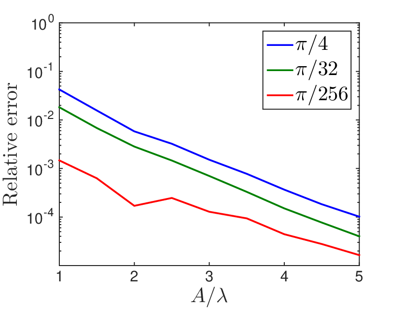
From the discussion above we see that, on the set $\{w=1\}$, the (superalgebraically high) accuracy of the solution $\phi^{w}$ of (10) does not deteriorate as the incidence angle $\alpha$ tends to zero. As shown in section 3 below, further, the solution $\phi^{w}$ can be used to produce the total field $u$ everywhere in space as well as the associated far field pattern. To conclude this section, in Figure 5 we demonstrate the fast and angle-independent convergence of $\phi^{w}$ to $\phi$: clearly the value of $A$ required to obtain an accurate approximation of the exact solution has been reduced substantially and the errors are uniformly small as the incidence angle decreases to zero.

An analysis similar to the one presented in section 2 for the density $\phi^{w}=[\varphi^{w},\psi^{w}]^{T}$ shows that substitution of $\phi=[\varphi,\psi]^{T}$ by $[w\varphi^{w}+(1-w)\varphi^{f},w\psi^{w}+(1-w)\psi^{f}]^{T}$ in (2) produces the fields $u_{1}$ and $u_{2}$ with superalgebraically high accuracy in a neighborhood of the region $\{w=1\}$ in $\mathbb{R}^{2}$, and, in particular, on a closed disc $D$ such as the one depicted in Figure 7. After some manipulations similar to those presented in the derivation of (11) above, the resulting formula can be re-expressed into a formula for the total field in terms of surface potentials defined on both $\Gamma$ and $\Pi$, namely

	$$\begin{split}u(\boldsymbol{x})=&\ \mathcal{D}_{1}\left[w\varphi^{w}\right](\boldsymbol{x})-\mathcal{S}_{1}\left[w\psi^{w}\right](\boldsymbol{x})-\mathcal{D}^{\Pi}_{1}\left[w\varphi^{f}\right](\boldsymbol{x})+\mathcal{S}^{\Pi}_{1}\left[w\psi^{f}\right](\boldsymbol{x})\\ &+\left\{\begin{array}[]{ll}u^{f}(\boldsymbol{x}),&\boldsymbol{x}\in\{x_{2}\geq 0\},\\ 0,&\boldsymbol{x}\in\{x_{2}<0\}\end{array}\right.\end{split}$$		(12a)
for $\boldsymbol{x}\in\Omega_{1}$, and
	$$\begin{split}u(\boldsymbol{x})=&\ -\mathcal{D}_{2}\left[w\varphi^{w}\right](\boldsymbol{x})+\mathcal{S}_{2}\left[\nu w\psi^{w}\right](\boldsymbol{x})+\mathcal{D}^{\Pi}_{2}\left[w\varphi^{f}\right](\boldsymbol{x})-\mathcal{S}^{\Pi}_{2}\left[\nu w\psi^{f}\right](\boldsymbol{x})\\ &+\left\{\begin{array}[]{ll}0,&\boldsymbol{x}\in\{x_{2}\geq 0\},\\ u^{f}(\boldsymbol{x}),&\boldsymbol{x}\in\{x_{2}<0\}\end{array}\right.\end{split}$$		(12b)

for $\boldsymbol{x}\in\Omega_{2}$.

Figure 6 compares the total field obtained by means of the WGF method and the layer-Green-function method [18] for the solution of the problem of scattering of a plane-wave by a semi-circular bump of radius $a=1$ in TE-polarization for wavenumbers $k_{1}=10$ and $k_{2}=15$ for $\alpha=-\pi/2$ and $\alpha=-\pi/6$ incidences. The WGF solution, in particular, was obtained from the solution of the integral equation (10) followed by evaluation of field values on the basis of (12b). Figures 6(c) and 6(f), which display the absolute value of the difference of the total fields computed using the WGF method and the layer-Green-function method on a bounded portion of the strip $\{w=1\}$ demonstrate the accuracy of the computed solutions in the near field.

As may be expected, however, formulae (12b) do not generally provide an accurate approximation of either far fields or near fields outside a neighborhood of $\Gamma_{A}$. In order to tackle this difficulty we consider the boundary $S$ of the disc $D$ mentioned above and depicted in Figure 7: $S$ encloses the portion of $\Gamma$ that differs from the flat interface $\Pi$ and, as indicated above, it lies within a fixed region within which superalgebraic convergence of the fields $u_{1}$ and $u_{2}$ takes place. Application of the Green identities, integrating over the region exterior to $S$ and utilizing the layer Green function leads to the following integral representation of scattered field $u^{s}=u-u^{f}$:

$$u^{s}(\boldsymbol{x})=\int_{S}\left\{\frac{\partial G^{1}_{2}}{\partial n_{\boldsymbol{y}}}(\boldsymbol{x},\boldsymbol{y})u^{s}(\boldsymbol{y})-G^{1}_{2}(\boldsymbol{x},\boldsymbol{y})\frac{\partial u^{s}}{\partial n}(\boldsymbol{y})\right\}\,\text{d}s_{\boldsymbol{y}}$$

(13)

outside the region enclosed by $S$, where $G_{2}^{1}$ denotes the layer Green function for the Helmholtz equation with wavenumbers $k_{1}$ in $\{x_{2}\geq 0\}$ and $k_{2}$ in $\{x_{2}<0\}$ that satisfies homogeneous transmission conditions on the flat interface $\Pi$ (see Appendix A). Note that the scattered field $u^{s}$ and its normal derivative on $S$ can be computed directly utilizing (12b) since by construction $S$ lies inside the region where (12b) provides an accurate approximation of the total field $u$.

The far-field pattern $u_{\infty}(\hat{\boldsymbol{x}})$, which is related to the scattered field by the asymptotic formula

$$u^{s}(\boldsymbol{x})=\frac{\operatorname{e}^{ik_{1}r}}{\sqrt{r}}u_{\infty}(\hat{\boldsymbol{x}})+\mathcal{O}(r^{-3/2}),\quad r=|\boldsymbol{x}|\rightarrow\infty,\quad\hat{\boldsymbol{x}}=\frac{\boldsymbol{x}}{|\boldsymbol{x}|},$$

can be obtained from (13) in a straightforward manner by replacing $G_{2}^{1}$ by its asymptotic expansion as $|\boldsymbol{x}|\rightarrow\infty$. The first order term of the asymptotic expansion of the Sommerfeld integrals $\Phi_{1}$ and $\Phi_{2}$ (equation 20) in a given direction $\hat{\boldsymbol{x}}=(\cos\alpha,\sin\alpha)$, $0<\alpha<\pi$ can be obtained by the method of steepest descent by taking into account the contribution of the saddle point [9] (branch point singularities and poles do not contribute to the first term of the asymptotic expansion of the two-layer Green function). Substitution of the result in equation (13) gives rise to the expression

$$u_{\infty}(\hat{\boldsymbol{x}})=\int_{S}\left\{\frac{\partial H}{\partial n_{\boldsymbol{y}}}(\hat{\boldsymbol{x}},\boldsymbol{y})u^{s}(\boldsymbol{y})-H(\hat{\boldsymbol{x}},\boldsymbol{y})\frac{\partial u^{s}}{\partial n}(\boldsymbol{y})\right\}\,\text{d}s_{\boldsymbol{y}}$$

(14)

for the far field $u_{\infty}(\hat{\boldsymbol{x}})$, where

	$\displaystyle H\left(\hat{\boldsymbol{x}},\boldsymbol{y}\right)=$	$\displaystyle\frac{\nu(k_{2}^{2}-k_{1}^{2})}{\sqrt{2\pi k_{1}}(1+\nu)}\frac{\operatorname{e}^{-ik_{1}\hat{\boldsymbol{x}}\cdot\boldsymbol{y}}\operatorname{e}^{-2y_{2}\eta_{1}+i\pi/4}}{\left(\eta_{2}+\eta_{1}\right)\left(\eta_{1}+\nu\eta_{2}\right)}+\frac{\operatorname{e}^{-ik_{1}\hat{\boldsymbol{x}}\cdot\boldsymbol{y}+i\pi/4}}{\sqrt{8\pi k_{1}}}+\left(\frac{1-\nu}{1+\nu}\right)\frac{\operatorname{e}^{-ik_{1}\hat{\bar{\boldsymbol{x}}}\cdot\boldsymbol{y}+i\pi/4}}{\sqrt{8\pi k_{1}}}$		(15a)
for $\boldsymbol{y}\in\{y_{2}\geq 0\}$ and
	$$H\left(\hat{\boldsymbol{x}},\boldsymbol{y}\right)=\frac{\nu k_{1}}{\sqrt{2\pi k_{1}}}\frac{\sin(\alpha-\beta)\operatorname{e}^{-ik_{1}\hat{\boldsymbol{x}}\cdot\boldsymbol{y}}\operatorname{e}^{y_{2}(\eta_{2}-\eta_{1})-i\pi/4}}{\eta_{1}+\nu\eta_{2}}$$			(15b)

for $\boldsymbol{y}\in\{y_{2}<0\}$, where $\hat{\bar{\boldsymbol{x}}}=\bar{\boldsymbol{x}}/|\boldsymbol{x}|=(\cos\alpha,-\sin\alpha)$, $\boldsymbol{y}=|\boldsymbol{y}|(\cos\beta,\sin\beta)$, $\eta_{1}=\gamma_{1}(k_{1}\cos(\alpha-\beta))$ and $\eta_{2}=\gamma_{2}(k_{1}\cos(\alpha-\beta))$ (see Appendix A for the definition of $\gamma_{1}$ and $\gamma_{2}$). Thus, unlike the layer Green function $G_{2}^{1}$ itself, the far field associated with $G_{2}^{1}$ can be computed inexpensively by means of the explicit expressions (15b). Figure 8 provides a comparison of the far-field patterns computed using the layer-Green-function method and the WGF method proposed in this paper for the example problem considered above in the present section 3.

In view of this discussion, equations (12b) and (13) can be used to accurately and efficiently evaluate near-fields and far-fields, respectively. These are typically the quantities of interest in scattering simulations involving layered media. The evaluation of the fields in an intermediate region, such as a domain outside the neighborhood of $\Gamma_{A}$ where (12b) yields an accurate approximation, can also be approximated efficiently on the basis of equation (13). Indeed, in such cases, for which source points $\boldsymbol{y}$ lie on $S$ and observation points $\boldsymbol{x}$ are at a certain distance away from $S$, the Sommerfeld integrals (20) and (22) (which contain highly oscillatory and/or exponentially decaying integrands) can be obtained by means of asymptotic numerical methods [2, 4] based on localization around critical points [9, 18].

This section illustrates the proposed methodology with a variety of numerical results concerning dielectric and conducting media, including relevant efficiency and accuracy studies.

In our first example we consider once again the configuration associated with Figure 5 (i.e. the problem of scattering by a semi-circular bump defect on a dielectric plane in TE-polarization). Here we compare the computing times required to create the systems of equations (which is the operation that dominates the computing time in all the examples considered) that stem from the discretization of the relevant integral equations by means of the WGF method (10) and the layer-Green-function method [18, Eq. 7]. Figure 9 displays the computing times for various wavenumbers $k_{1}$ and $k_{2}=2k_{1}$ for each method. The discretization density was held proportional to $k_{1}$ to properly resolve the oscillatory character of the integrands and the same discretization was used for both methods on the bump, allowing for a point by point comparison of the solutions. In all these examples the WGF method was optimized to produce a maximum error of approximately $5\times 10^{-5}$ in the computation of the density $\phi^{w}$ on the surface of the bump. Similarly, the key parameters in the implementation of layer-Green-function method (including the parameters associated to the numerical evaluation of the Sommerfeld integrals) were adjusted to yield the fastest possible solution within an error of $5\times 10^{-5}$. Note that the last data points around $k_{1}=8\pi\approx 25.1$ in Figure 9 (which is the last data point presented for the layer-Green-function method) shows that, for such frequencies the WGF is approximately three orders of magnitude faster than the layer-Green-function method [18].

The problem of scattering by the city-like structure depicted in Figure 10 is considered next. Figure 10 also displays the window function utilized in this example, which has been amplified by a factor 8 for visualization purposes. In contrast with the results presented previously in this paper, the case of TM-polarization is considered for this test. In order to properly account for the singular behavior of the fields near corners, the necessary graded meshes were generated utilizing the value $p=4$ in the method described in [13]. Table 1 reports the computing times required to form the relevant system matrices for both the WGF method and the layer-Green-function method. Both solvers were optimized to produce a maximum error of $5\times 10^{-3}$ in the solutions of the integral equation, and the same computational grids were utilized to discretize the buildings for both methods.

Table 1 compares the computing times required by the WGF method and the layer-Green-function method for two values of $k_{2}$. In particular we note that, not only is the new method much faster than the previous approach, but also that the speed-up factor grows: a speed up factor in the hundreds for the value $k_{2}=2\pi$ is doubled as $k_{2}$ is itself doubled to the value $k_{2}=4\pi$. Additionally, application of the layer-Green-function method in this context requires use of fictitious curves underneath each building [18] each one of which (curves) must itself be discretized, while the WGF method requires discretization of the ground between the buildings and in the region where the windowing takes place. In the present case the layer-Green-function method produced a system of 2384 unknowns while the WGF method produced a nearly identical sized system of 2406 unknowns. At higher frequencies, the WGF method requires fewer unknowns than the layer-Green-function method, since, as demonstrated in Table 2, at higher frequencies the width of the windowing function can be decreased while maintaining accuracy.

As an additional example we consider once again the city-like structure depicted in Figure 10 but assuming an absorbing media in the ground and buildings: here we thus take $k_{1}=2\pi$ and $k_{2}=4\pi(1+i/100)$. Figure 11 demonstrates the convergence of both the naive windowing algorithm (6) and the full WGF method (10). The advantages provided by the full WGF approach can be appreciated clearly in this figure: in the naive method convergence near grazing is extremely slow while for the full WGF method the convergence is actually faster near grazing than for non-grazing configurations. In particular, the WGF method requires no more than 5 wavelengths of ground for a full four digits of accuracy, independently of the incidence angle.

For our last numerical example we consider an obstacle above the ground, but not connected to it, with a finite number of indentations under the ground level. Figure 12 displays the geometry under consideration, together with a selection of window function which yields an error of approximately 1% in the integral equation solution and corresponding near fields for a plane-wave illumination with incidence angle equal to $\alpha=-\pi/8$ from the horizontal under TE polarization. Once again, as demonstrated in Figure 13 exponential convergence is observed as $A/\lambda$ grows.

The authors gratefully acknowledge support from the Air Force Office of Scientific Research and the National Science Foundation.

References

- [1] M. I. Aksun, A. Alparslan, and K. A. Michalski. Current status of closed-form Green’s functions in layered media composed of natural and artificial materials. 2009 International Conference on Electromagnetics in Advanced Applications, 2009.
- [2] A. Asheim and D. Huybrechs. Asymptotic Analysis of Numerical Steepest Descent with Path Approximations. Foundations of Computational Mathematics. The Journal of the Society for the Foundations of Computational Mathematics, 10(6):647–671, Dec. 2010.
- [3] O. P. Bruno and B. Delourme. Rapidly convergent two-dimensional quasi-periodic Green function throughout the spectrum—including Wood anomalies. Journal of Computational Physics, 262:262–290, 2014.
- [4] O. P. Bruno, C. Geuzaine, J. Monro, and F. Reitich. Prescribed error tolerances within fixed computational times for scattering problems of arbitrarily high frequency: the convex case. Philosophical Transactions of the Royal Society of London. Series A: Mathematical, Physical and Engineering Sciences, 362(1816):629–645, 2004.
- [5] O. P. Bruno and C. Pérez-Arancibia. Windowed Green Function method for layered-media scattering: Theoretical considerations. In preparation, 2015.
- [6] W. Cai. Algorithmic issues for electromagnetic scattering in layered media: Green’s functions, current basis, and fast solver. Advances in Computational Mathematics, 16:157–174, 2002.
- [7] W. Cai and T. Yu. Fast Calculations of Dyadic Green’s Functions for Electromagnetic Scattering in a Multilayered Medium. Journal of Computational Physics, 165:1–21, 2000.
- [8] W. C. Chew. Waves and fields in inhomogeneous media, volume 522. IEEE press New York, 1995.
- [9] T. J. Cui and W. C. Chew. Efficient evaluation of Sommerfeld integrals for TM wave scattering by buried objects. Journal of Electromagnetic Waves and Applications, 12(5):607–657, 1998.
- [10] T. J. Cui and W. C. Chew. Fast evaluation of Sommerfeld integrals for EM scattering and radiation by three-dimensional buried objects. IEEE Transactions on Geoscience and Remote Sensing, 37(2):887–900, 1999.
- [11] J. A. DeSanto and P. A. Martin. On the derivation of boundary integral equations for scattering by an infinite one-dimensional rough surface. J. Acoust. Soc. Am, 102(1):67–77, July 1997.
- [12] R. Kittappa and R. E. Kleinman. Acoustic Scattering by Penetrable Homogeneous Objects. Journal of Mathematical Physics, 16(2):421–432, 1975.
- [13] R. Kress. A Nyström method for boundary integral equations in domains with corners. Numerische Mathematik, 58(1):145–161, 1990.
- [14] A. Meier and S. N. Chandler-Wilde. On the stability and convergence of the finite section method for integral equation formulations of rough surface scattering. Mathematical Methods in the Applied Sciences, 24(4):209–232, 2001.
- [15] D. Miret, G. Soriano, and M. Saillard. Rigorous Simulations of Microwave Scattering From Finite Conductivity Two-Dimensional Sea Surfaces at Low Grazing Angles. IEEE Transactions on Geoscience and Remote Sensing, 52(6):3150–3158, 2014.
- [16] J. A. Monro Jr. A Super-Algebraically Convergent, Windowing-Based Approach to the Evaluation of Scattering from Periodic Rough Surfaces. Ph.D. Thesis, Caltech, 2008.
- [17] M. Paulus, P. Gay-Balmaz, and O. Martin. Accurate and efficient computation of the Green’s tensor for stratified media. Physical Review E, 62(4):5797, 2000.
- [18] C. Pérez-Arancibia and O. P. Bruno. High-order integral equation methods for problems of scattering by bumps and cavities on half-planes. Journal of the Optical Society of America A, 31(8):1738–1746, Aug. 2014.
- [19] M. Saillard and G. Soriano. Rough surface scattering at low-grazing incidence: A dedicated model. Radio Science, 46(5), Oct. 2011.
- [20] A. Sommerfeld. Über die Ausbreitung der Wellen in der drahtlosen Telegraphie. Annalen der Physik, 333(4):665–736, 1909.
- [21] P. Spiga, G. Soriano, and M. Saillard. Scattering of Electromagnetic Waves From Rough Surfaces: A Boundary Integral Method for Low-Grazing Angles. IEEE Transactions on Antennas and Propagation, 56(7):2043–2050, July 2008.
- [22] Z. Zhao, L. Li, J. Smith, and L. Carin. Analysis of scattering from very large three-dimensional rough surfaces using MLFMM and ray-based analyses. Antennas and Propagation Magazine, IEEE, 47(3):20–30, June 2005.