Influence of a plasma on the shadow of a spherically symmetric black hole
Abstract
We analytically calculate the influence of a plasma on the shadow of a black hole (or of another compact object). We restrict to spherically symmetric and static situations, where the shadow is circular. The plasma is assumed to be non-magnetized and pressure-less. We derive the general formulas for a spherically symmetric plasma density on an unspecified spherically symmetric and static spacetime. Our main result is an analytical formula for the angular size of the shadow. As a plasma is a dispersive medium, the radius of the shadow depends on the photon frequency. The effect of the plasma is significant only in the radio regime. The formalism applies not only to black holes but also, e.g., to wormholes. As examples for the underlying spacetime model, we consider the Schwarzschild spacetime and the Ellis wormhole. In particular, we treat the case that the plasma is in radial free fall from infinity onto a Schwarzschild black hole. We find that for an observer far away from a Schwarzschild black hole the plasma has a decreasing effect on the size of the shadow. The perspectives of actually observing the influence of a plasma on the shadows of supermassive black holes are discussed.
- PACS numbers
-
04.20.-q – 98.62.Sb – 98.62.Mw – 98.35.Jk
pacs
?????? - ??????pacs
?????? - ??????I Introduction
In the last twenty years increasing evidence has been found for the existence of a supermassive black hole at the center of our galaxy. It is expected that a distant observer should “see” this black hole as a dark disk in the sky which is known as the “shadow”. It is sometimes said that the shadow is an image of the event horizon, and the size of the shadow is estimated by the angle under which the observer would see the horizon according to Euclidean geometry. Actually, the boundary of the shadow corresponds to light rays that asymptotically approach the photon sphere (at in the Schwarzschild case) and not the horizon (at in the Schwarzschild case). Moreover, light rays do not follow straight lines in Euclidean geometry but they are bent. For these two reasons, the angular diameter of the shadow is actually bigger than the naive Euclidean estimate suggests. For the black hole at the center of our galaxy, it amounts to about 53 as whereas the Euclidean estimate gives only about 20 as. At present, two projects are under way to observe this shadow which would give important information on the compact object at the center of our galaxy. These projects, which are going to use (sub)millimeter VLBI observations with radio telescopes distributed over the Earth, are the Event Horizon Telescope (http://eventhorizontelescope.org) and the BlackHoleCam (http://blackholecam.org).
On the theoretical side, the shadow is defined as the region of the observer’s sky that is left dark if there are light sources distributed everywhere but not between the observer and the black hole. For a non-rotating black hole, the shadow is a circular disk. For a Schwarzschild black hole the angular diameter of the shadow was calculated, as a function of the mass of the black hole and of the radius coordinate where the observer is situated, by Synge [1]. (Synge did not use the word “shadow”. He calculated what he called the “escape cones” of light. However, the complement of the opening angle of the escape cone at the observer gives exactly the diameter of the shadow.) For a rotating black hole the shadow is no longer circular. The first to correctly calculate the shape of the shadow of a Kerr black hole was Bardeen [2]. More generally, the shape and the size of the shadow can be calculated analytically for the whole class of Plebański-Demiański spacetimes [3, 4]. All these calculations are based on the assumption that light propagates along lightlike geodesics, without being influenced directly by matter. If such an influence is to be taken into account, one usually resorts to numerical calculation. In particular, Falcke, Melia and Agol [5] have numerically simulated the visual appearance of the black hole at the center of our galaxy, assuming that it is a Kerr black hole, with scattering and the presence of emission regions between the observer and the black hole taken into account (at 0.6 and 1.3 mm wavelengths). Sophisticated ray tracing programs have been written for producing realistic images of a black hole surrounded by an accretion disk, e.g. for the movie Interstellar. The numerical techniques used for this movie are described in detail, along with a review of earlier work, by James et al. [6].
While the purely geometric calculation of the shadow can be done analytically, at least for spacetimes in which the equation for lightlike geodesics is completely integrable, virtually all of the work that takes the influence of matter into account was based on numerics so far. In this paper we want to take the first steps towards an investigation of the shadow in matter based on analytical calculations. It is clear that this can be done only for highly idealized situations, but nonetheless we think that it is worthwile to do so. In contrast to numerical simulations, which can depict the situation only for a particular choice of the parameters involved, analytical results demonstrate how exactly an effect depends on these parameters and they bring out the general features more clearly. Also, analytical results are useful for testing numerical codes. In this paper we begin with the simplest non-trivial case: We want to analytically calculate the influence of a non-magnetized pressure-less plasma on the size of the shadow of a non-rotating black hole.
A plasma is a dispersive medium, i.e., the light rays deviate from lightlike geodesics in a way that depends on the frequency. The Hamiltonian for the light rays can be derived from Maxwell’s equations where the source of the electromagnetic field consists of two charged fluids, one modelling the ions and the other the electrons. For a plasma on a curved background, the transition from Maxwell’s equations to ray optics has to be done by a two-scale method. A rigorous derivation of the Hamiltonian for light rays was provided by Breuer and Ehlers [7, 8] who considered a magnetized pressure-less plasma. For the much simpler case of a non-magnetized pressure-less plasma, a similar derivation can be found in Perlick [9]. In the latter case the equation of light rays can be fully characterized by a scalar, i.e. direction-independent, index of refraction which is a function of the spacetime point and of the frequency. Then the resulting equation of motion for light rays belongs to a class that was studied in the text-book by Synge [10]. The resulting formula for the deflection angle of light in a plasma whose density is a function of the radius coordinate was calculated in the Schwarzschild spacetime (and more generally in the equatorial plane of the Kerr metric) by Perlick [9]. The same result was found and further discussed by Bisnovatyi-Kogan and Tsupko [11], [12], [13]. Morozova et al. [14] generalized the calculation to the Kerr metric off the equatorial plane, assuming that the black hole is slowly rotating. For recent suggestions of how the effects of a plasma on light rays could actually be observed we refer to Er and Mao [15] and to Rogers [16].
In this paper we calculate the angular diameter of the shadow for a non-rotating black hole that is surrounded by a non-magnetized pressure-less plasma. Although we are mainly interested in the Schwarzschild case, in large parts of the paper we work in an unspecified spherically symmetric and static spacetime, so the results can be applied, e.g., also to charged black holes or to wormholes.
In our work the plasma manifests itself as a refractive and dispersive medium, which leads to a change of the light rays in comparison with vacuum. As a result, the geometrical size of the shadow is changed. We do not take into account the processes of absorption and scattering of the photons by plasma electrons. Also, we neglect the gravitational field of the plasma particles.
The paper is organized as follows. In Section II we work out the equation of motion for light rays in a plasma on a spherically symmetric and static spacetime. In Section III we determine the circular light orbits which are of crucial relevance for the formation of the shadow. In Section IV we calculate the angular diameter of the shadow. We specify the results in Section V to the case of a low-density plasma and in Section VI to the case that the plasma has the particular density profile that corresponds to spherically symmetric accretion of a dust onto a Schwarzschild black hole. In the same section we also discuss the perspectives of actually observing the influence of a plasma on the shadow of a supermassive black hole.
We use units such that , so the Schwarzschild radius is . Our choice of signature is . We use Einstein’s summation convention for latin indices which take the values .
II Equations of motion for light rays in a non-magnetized plasma
We consider a spherically symmetric and static metric
| (1) |
where , and are positive. We are mainly interested in the case of a Schwarzschild black hole but for the time being there is no need for specifying the metric any further.
We assume that the spacetime is filled with a non-magnetized cold plasma whose electron plasma frequency is a function of the radius coordinate only,
| (2) |
Here is the charge of the electron, is the electron mass, and is the number density of the electrons in the plasma. The refraction index of this plasma depends on the radius coordinate and on the frequency of the photon as it is measured by a static observer,
| (3) |
Because of the spherical symmetry we may restrict to the equatorial plane , . Then the Hamiltonian for light rays in the plasma reads
| (4) |
For a derivation of the Hamiltonian (4) from Maxwell’s equations with a two-fluid source we refer to the literature given in the introduction.
The light rays are the solutions to Hamilton’s equations
| (5) |
which in this case read
| (6) |
| (7) |
| (8) | |||
| (9) |
| (10) |
| (11) |
with , i.e.
| (12) |
Here a dot means differentiation with respect to an affine parameter , and a prime means differentiation with respect to .
¿From (6) and (7) it follows that and are constants of motion. We write . If has been fixed and if for , which is the case if the spacetime is asymptotically flat, the frequency measured by a static observer becomes a function of by the gravitational redshift formula,
| (13) |
By (12), a light ray with constant of motion is restricted to the region where
| (14) |
The restriction (14) physically means that the photon frequency at a given point, , must be bigger than the plasma frequency, , at the same point. This is always true for light propagation in a plasma.
To derive the orbit equation, we use (10) and (11) to find
| (15) |
Upon substituting for from (12), this results in
| (16) |
where we have defined the function
| (17) |
In general, the orbit has to be decomposed into sections where is increasing as a function of and sections where it is decreasing, and the sign in (16) has to be chosen appropriately. For a light ray that comes in from infinity, reaches a minimum at a radius , and goes out to infinity again, integration over the orbit gives the formula for the bending angle, ,
| (18) |
As corresponds to the turning point of the trajectory, the condition has to hold. This equation relates to the constant of motion ,
| (19) |
Then the deflection angle can be rewritten as a function of only and (for a given plasma distribution) as
| (20) |
Example : Schwarzschild spacetime
For the Schwarzschild spacetime,
| (21) |
the function specifies to
| (22) |
Then the bending angle reads
| (23) | |||
This formula for the bending angle in a plasma on Schwarzschild spacetime was derived in [9]. In [13] it was rederived using Synge’s approach and rewritten in terms of an elliptic integral for a homogeneous plasma; there also the strong deflection limit () was investigated.
Example : Ellis wormhole
As a second example we choose the Ellis wormhole [32] which is a traversible wormhole of the Morris-Thorne class [34]. It is true that the existence of such wormholes is questionable because they need exotic matter [34] and, at least for a certain kind of perturbations, it has been shown that the Ellis wormhole is unstable [35, 36, 37]. On the other hand, wormholes have met with great interest because they make time travel possible and the Ellis wormhole is an instructive example for illustrating the applicability of our results. In this case the metric coefficients are
| (24) |
where the coordinate ranges from to and is a constant that determines the radius of the “neck” of the wormhole. Note that this is an example of a spherically symmetric and static spacetime where we cannot make a transformation of the radius coordinate, , such that . The reason is that the function has vanishing derivative at (i.e., at the “neck”), so the desired transformation fails to be a good coordinate transformation on any radius interval that contains the point . For the Ellis wormhole the function reads
| (25) |
and the bending angle is given by
| (26) | |||
III Circular light orbits
We now derive the condition for cicular light orbits which will be crucial for determining the shadow. Along a circular light orbit we must have and . The first condition, by (11), implies ; from (12) we get the equation
| (27) |
On the other hand, (11) implies
| (28) |
¿From this equation we read that together with leads to , and from (8) we get the second equation for circular light orbits,
| (29) |
We solve each of these two equations (27) and (29) for ,
| (30) |
| (31) |
Subtracting these two equations from each other yields, after some elementary re-arrangements, the equation for the radius of a circular light orbit in the form
| (32) |
with the function from (17). Any solution of (32) determines the radius of a photon sphere. If a light ray starts tangentially to such a sphere it will stay on a circular path with radius forever. If the spacetime is asymptotically flat, and if for , the outermost photon sphere is always unstable with respect to radial perturbations. This means that the circular photon orbits in this photon sphere can serve as limit curves for light rays that approach them asymptotically. The radius of the outermost photon sphere is the critical value of the minimal radius mentioned above. If a light ray comes in from infinity and reaches a minimum radius bigger than , it will go out to infinity again. The case corresponds to a light ray that spirals asymptotically towards a circular photon orbit in the sphere of radius . All other rays cross the photon sphere and we exclude the case that they can come back. The latter case can occur only if there is a second photon sphere.
In the vacuum case, , the condition for a circular light orbit in an unspecified spherically symmetric and static spacetime was first given by Atkinson [33]. It is easy to check that our condition (32) reduces, indeed, to Atkinson’s if .
Example : Schwarzschild spacetime
For the Schwarzschild spacetime, where is given by (22), condition (32) for a photon sphere reads
| (33) |
For the special case that depends on via a power law, this condition was already derived by Rogers [16]. If there is no plasma, , (33) gives the well-known result . For the sake of curiosity, notice that (33) is identically satisfied if
| (34) |
| (35) |
with a positive constant . For this particular density profile of the plasma, there is a circular photon orbit with constant of motion at any radius for which
| (36) |
Example : Ellis wormhole
For the Ellis wormhole, is given by (25) and condition (32) for a photon sphere reads
| (37) |
Without a plasma, , there is a unique photon sphere at the neck of the wormhole, . The same is true for a homogeneous plasma, . However, in an inhomogeneous plasma there may be arbitrarily many photon spheres. For an observer at a large positive coordinate, the outermost photon sphere is relevant for the formation of the shadow which will be discussed in the next section.
IV Radius of the shadow
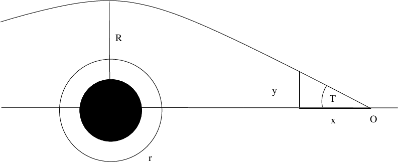
The shadow of a spherically symmetric and static black hole is defined in the following way, see Fig. 1. Consider light rays sent from an observer at radius coordinate into the past. As we want to take the influence of a plasma into account, by a light ray we mean a solution to the equations of motion discussed in Section II. These light rays can be divided into two classes: Light rays of the first class go to infinity after being deflected by the black hole. Light rays of the second class go towards the horizon of the black hole. If we assume that there are no light sources between the observer and the black hole, initial directions of the second class correspond to darkness on the observer’s sky. This dark circular disk on the observer’s sky is called the shadow of the black hole. The boundary of the shadow is determined by the initial directions of light rays that asymptotically spiral towards the outermost photon sphere. Here it is crucial that the light rays in the photon sphere are unstable with respect to radial perturbations because otherwise they could not serve as limit curves. For this reason, the construction of the shadow works for any spherically symmetric and static spacetime that admits an unstable photon sphere. This includes not only black holes but also, e.g., wormholes. We have already mentioned that in a spherically symmetric and static spacetime that is asymptotically flat the outermost photon sphere is always unstable, provided that the plasma density tends to zero for . We will now calculate, for this situation, the angular radius of the shadow. The observer is assumed to be static somewhere between the outermost photon sphere and infinity.
We consider a light ray that is sent from the observer’s position at into the past under an angle with respect to the radial direction. ¿From Fig. 1 we read that is given by
| (38) |
If the light ray goes out again after reaching a minimum radius , the orbit equation (16) can be rewritten, with the help of (19), as
| (39) |
For the angle we obtain
| (40) |
Using
| (41) |
we get
| (42) |
The boundary of the shadow is determined by light rays that spiral asymptotically towards a circular light orbit at radius . Therefore the angular radius of the shadow is given by sending in (42),
| (43) |
where is given by the formula (17).
For many applications we may assume that the observer is in a region where the plasma density is negligibly small. Then (17) implies
| (44) |
and (43) reduces to
| (45) |
This demonstrates that, under the assumptions stated, the plasma always has a decreasing effect on the size of the shadow.
We emphasize that the preceding calculation applies not only to black holes but also to other spherically symmetric and static spacetimes with an unstable photon sphere, e.g. to ultracompact stars and to wormholes. As long as there is no light coming from the direction of the central object to the observer (which means, in particular, that the central object must not have a bright surface), these objects would cast a shadow in the same way as a black hole.
Let us summarize the results of this section. To find for a given metric of the form (1), a given plasma concentration , a given photon frequency at infinity and a given observer position , we have to calculate using eq.(32) and to substitute the result into formula (43). Note that the photon frequency at the observer position is according to (13).
Example : Schwarzschild spacetime
For the Schwarzschild case (43) specifies to
| (46) |
where has to be determined from (33). In Section VI below we will evaluate this equation for a particular plasma density profile. For vacuum, , our consideration gives
| (47) |
This is Synge’s [1] formula for the radius of the shadow of a Schwarzschild black hole which was mentioned already in the introduction.
Example : Ellis wormhole
We now calculate the radius of the shadow for the Ellis wormhole. In this case, our assumption of no light coming towards the observer from the direction of the central object means, in particular, that there are no light sources in the region . For the Ellis wormhole, the function is given by (25), so the equation (43) for the angular radius of the shadow specifies to
| (48) |
For a homogeneous plasma, , we have and thus
| (49) |
so a homogeneous plasma has no influence on the size of the shadow.
V The shadow in a low-density plasma
If the plasma frequency is much smaller than the photon frequency, the equations for the photon sphere and for the radius of the shadow can be linearized about the corresponding values for vacuum light rays. To work this out, we rewrite (17) as
| (50) |
where
| (51) |
Here we have introduced a book-keeping parameter which will be set equal to unity after all equations have been linearized with respect to .
The equation for a photon sphere, (32), now reads
| (52) |
We write the solution to this equation in the form
| (53) |
where is a solution in the case without plasma, i.e.,
| (54) |
After inserting these expressions into (52) and comparing coefficients of we find
| (55) |
Depending on the signs of and , this expression can be positive or negative, i.e., the plasma can shift the photon sphere inwards or outwards.
We now insert the expansion (53) into the equation for the shadow (43). If we neglect all terms of quadratic and higher order in , and set equal to unity again, we find
| (56) |
Note that has dropped out from the equation for to within this order. According to (56), the plasma has a decreasing effect on the shadow as long as .
Let us summarize the results of this section. To find the radius of the photon sphere for a given metric (1), a given photon frequency at infinity , and a given plasma frequency that satisfies the condition one has to proceed in the following way: Write down the functions and , see (51); calculate from (54) and from (55); then calculate according to (53) with . To find the angular radius of the shadow for a given observer position in this case, we have to insert into (56).
Example : Schwarzschild spacetime
As an example of the approximation formalism developed in this section, we consider the Schwarzschild spacetime for the case that the plasma electron density is given by a power law,
| (57) |
where and are positive dimensionless constants. Then and
| (58) |
i.e., depending on the density profile the radius of the photon sphere may become smaller () or bigger () than . In the case that we obtain . Note that in this case the equation for the photon sphere can be solved exactly and gives the same result, . The first-order equation for the radius of the shadow, (56), yields
| (59) | |||
If the observer is far away from the black hole, , this can be simplified to
| (60) |
Example : Ellis wormhole
For the Ellis wormhole,
| (61) |
With , the first-order approximation yields
| (62) |
VI Spherically symmetric accretion of a plasma onto a Schwarzschild black hole
In this section we consider in greater detail the special case that the underlying spacetime is the Schwarzschild spacetime and that the plasma electron density corresponds to spherically symmetric accretion of dust. As usual, we use the word “dust” as a synonym for a pressure-less perfect fluid. Vanishing pressure implies that the flow lines are geodesics, i.e., that the fluid particles are freely falling. Note that for our plasma model the Hamiltonian and, thus, the equations of motion for light rays do not depend on the velocity of the plasma. This is, of course, different for other types of media, see Synge’s book [10]. In the case of an infalling plasma we have to determine the plasma density which is the only quantity that enters into the equation for the plasma frequency.
We start out from the continuity equation
| (63) |
Here is the rest-mass density of the plasma, is the 4-velocity, and is the determinant of the metric. For the sake of simplicity, we consider a neutral hydrogen plasma and we assume that the electrons have the same 4-velocity as the protons. As the electron mass is negligibly small in comparison to the proton mass, can be written as where is the proton rest mass and is the number density of the protons (which, as the plasma is assumed to be neutral, coincides with the number density of the electrons).
For spherically symmetric and stationary accretion in the Schwarzschild spacetime the continuity equation reduces to
| (64) |
Integration gives
| (65) |
where is a stationary mass flux.
We assume that the particles are dropped in radial free fall from rest at infinity, i.e., that our plasma is so “cold” that the pressure can be neglected. Then the integral curves of are radial geodesics, so the radial component of the 4-velocity is [20]
| (66) |
Thereupon, eq. (65) gives us the rest-mass density,
| (67) |
Equations (66) and (67) also follow from Michel’s pioneering paper [21] on fully relativistic spherically symmetric accretion where we have to specify Michel’s equations (9) and (10) to the case of a dust.
The rest-mass density gives us the ratio of frequencies
| (68) |
where
| (69) |
For this function , the angular radius (46) of the shadow is plotted, as a function of for different observer positions, in Fig. 2.
Assuming that the approximation of a low-density plasma is justified, we can use formula (59) and find
| (70) | |||
In this case the function which enters into (56) is equal to zero when and it takes its maximum when . When , the function is negative. Therefore, if the approximation of a low-density plasma is justified, the shadow becomes bigger if and it becomes smaller if .

As an aside, we mention that the 4-velocity component directly gives the velocity of the infalling particles as measured by a static observer. To demonstrate this, following [20] (see also [22]), we first observe that (66) together with the normalization condition implies that
| (71) |
hence
| (72) |
For a static observer at radius coordinate , a coordinate time interval corresponds to a proper time interval
| (73) |
On the other hand, a radial coordinate separation corresponds to a proper radial distance equal to
| (74) |
As a consequence, the velocity of the radially infalling particle, as measured by a static observer at , is given by
| (75) |
We will now use the results of this section for estimating the numerial values of the plasma effects on the shadow of the supermassive black holes at the center of our galaxy and of M87.
For these applications we can always use the formulas with , so the angular radius of the shadow (60) can be written as
| (76) |
was defined in (69). For estimating the plasma correction numerically, we re-express all quantities in Gaussian cgs units, i.e., we restore factors of and . Then reads
| (77) |
The mass accretion rate can be estimated via the observed luminosity of the galactic center. We write
| (78) |
where is a non-dimensional coefficient characterizing the accretion efficiency. We obtain for the correction due to the presence of the plasma:
| (79) |
Note that the circular frequency is connected with the ordinary frequency by the usual relation, , and that in the expression for we can assume, as a valid approximation, that is related to the wavelength by the vacuum relation .
The value of depends on the specific model of accretion. For estimations we consider (see [23], [24]) and (see [25]).
Let us consider the galactic center source Sgr A*. For estimations we put , kpc (see [26], [27]). Then Synge’s formula (47) gives for the angular radius of the shadow in vacuum a value of as, i.e., a diameter of about 53 as which is expected to be resolvable with Very Long Baseline Interferometry (VLBI) soon [28], [29]. By contrast, a naive Euclidean estimate of the horizon size, , yields as, i.e., a diameter of about 20 as, as was already mentioned in the introduction. For a rotating (Kerr) black hole, the shadow is flattened on one side, but its vertical diameter is still given by Synge’s formula if , see [4].
For estimating the correction we use (see, for example [30]). For mm we obtain:
| (80) |
Note that observations of the shadow are planned in the (sub)millimeter regime because at wavelengths of more than about 1.3 mm it is expected that the shadow is washed out by scattering [5]. We see that in this regime the effect of a plasma is rather small, for the chosen values of . However, for bigger radio wavelengths the effect can be significant. For cm we obtain:
| (81) |
We now turn to the galactic center source M87. For estimations we put , Mpc, ergs s-1 (see, for example [30]). Then Synge’s formula leads to an angular radius of the shadow in vacuum of as.
For mm we obtain:
| (82) |
For cm we obtain:
| (83) |
VII Conclusions
In this paper the first steps towards an investigation of the shadow in the presence of matter based on analytical calculations have been taken. We have analytically calculated the influence of a non-magnetized pressure-less plasma on the angular size of the shadow. It was our goal to derive all relevant formulas for an unspecified spherically symmetric and static spacetime, before specializing to the case of a Schwarzschild black hole. The gravitational field was not supposed to be weak. We have worked in the frame-work of geometrical optics; in this approximation the presence of the plasma leads to a change of the geometrical size of the shadow via a change of the light rays in this medium.
The equation of motion for light rays in a plasma with a spherically symmetric density distribution on a spherically symmetric and static spacetime (1) has been derived, see (16). In particular, the formula for the photon deflection angle has been shown for unbound orbits, see (20). We have also found the radii of the circular light orbits (radii of the photon spheres), see (32). The central result of our paper is an analytical formula for the angular size of the shadow, see (43). 11 1 Soon after a preprint of the present paper was made public on the arXiv [17], a paper by Atamurotov and Ahmedov [18] appeared, again on the arXiv, where the shadow was calculated for the case of a homogeneous plasma. Their results are in obvious disagreement with ours if the latter are specialized to the case of a homogeneous plasma. The reason is in the fact that they erroneously treated the index of refraction as a constant. Actually, the index of refraction involves the plasma density, which is constant in a homogeneous plasma, and the photon frequency, which in a gravitational field depends on the space point. Therefore, the index of refraction is not a constant for a homogeneous plasma. This has the consequence that in the Schwarzschild spacetime the photon sphere in a homogeneous plasma is different from the vacuum case. In the meantime, a strongly revised version of their paper appeared in PRD [19] where they are now considering a plasma density proportional to .
Special attention was given to the realistic case when the plasma frequency is much smaller than the photon frequency, see Section V. We have shown that in this case the plasma has a decreasing effect on the size of the shadow provided that the plasma density is higher at the photon sphere than at the observer position, see (56). In particular, a simple formula for the size of the shadow was presented for the case of a power-law density distribution and an observer at a large distance, see (60).
In the presence of a plasma the size of the shadow depends on the wavelength at which the observation is made, in contrast to the vacuum case where it is the same for all wavelengths. For the underlying spacetime we have treated two examples, the Schwarzschild black hole and the Ellis wormhole. In particular, the case of spherically symmetric accretion of plasma onto a Schwarzschild black hole was considered in detail, see Section VI. We have found that for an observer far away from the Schwarzschild black hole the plasma makes the shadow smaller. As examples, we have considered Sgr A* and M87. For the specific accretion model used here we have found that the effect of the presence of a plasma on the size of the shadow can be significant only for wavelengths of at least a few centimeters. At such wavelengths the observation of the shadow is made difficult because of scattering.
Apart from considering more complicated plasma models, an obvious next step would be to generalize the analysis to the case of axially symmetric and stationary situations to include rotating black holes. Then the shadow is no longer circular, and the plasma has an effect not only on its size but also on its shape. We are planning to work out the details in future work.
Acknowledgments
VP wishes to thank Deutsche Forschungsgemeinschaft for financial support under Grant No. LA 905/14-1 and the Dynasty Foundation for financing his visit to Moscow where part of this work was carried through. Also, VP acknowledges support from the Deutsche Forschungsgemeinschaft within the Research Training Group 1620 “Models of Gravity”. The results for the Schwarzschild black hole were obtained by OYuT and GSBK, and this part of work was financially supported by Russian Science Foundation, Grant No. 15-12-30016.
References
- [1] J. L. Synge, Mon. Not. Roy. Astron. Soc. 131, 463 (1966)
- [2] J. M. Bardeen, in Black Holes, edited by C. DeWitt and B. DeWitt (Gordon and Breach, New York, 1973), p. 215
- [3] A. Grenzebach, V. Perlick, and C. Lämmerzahl, Phys. Rev. D 89, 124004 (2014)
- [4] A. Grenzebach, V. Perlick, and C. Lämmerzahl, Int. J. Mod. Phys. D 24, 1542024 (2015)
- [5] H. Falcke, F. Melia, and E. Agol, Astrophys. J. 528, L13 (2000)
- [6] O. James, E. Tunzelmann, P. Franklin, and K. Thorne, Class. Quantum Grav. 32, 065001 (2015)
- [7] R. A. Breuer and J. Ehlers, Proc. Roy. Soc. London A 370, 389 (1980)
- [8] R. A. Breuer and J. Ehlers, Proc. Roy. Soc. London A 374, 65 (1981)
- [9] V. Perlick, Ray Optics, Fermat’s Principle, and Applications to General Relativity, (Springer, Berlin, 2000)
- [10] J. L. Synge, Relativity. The general theory, (North-Holland, Amsterdam, 1960)
- [11] G. S. Bisnovatyi-Kogan and O. Yu. Tsupko, Gravitation and Cosmology 15, 20 (2009)
- [12] G. S. Bisnovatyi-Kogan and O. Yu. Tsupko, Mon. Not. Roy. Astr. Soc. 404, 1790 (2010)
- [13] O. Yu. Tsupko and G. S. Bisnovatyi-Kogan, Phys. Rev. D 87, 124009 (2013)
- [14] V. Morozova, B. Ahmedov, and A. Tursunov, Astrophys. Space Sci. 346, 513 (2013)
- [15] X. Er and S. Mao, Mon. Not. Roy. Astron. Soc. 437, 2180 (2013)
- [16] A. Rogers, gravitational lensing within plasma. Mon. Not. Roy. Astron. Soc. 451, 4536 (2015)
- [17] V. Perlick, O. Yu. Tsupko and G. S. Bisnovatyi-Kogan, arXiv:1507.04217v1 (2015)
- [18] F. Atamurotov, B. Ahmedov, arXiv:1507.08131v1 (2015)
- [19] F. Atamurotov, B. Ahmedov, A. Abdujabbarov, Phys. Rev. D 92, 084005 (2015)
- [20] M. P. Hobson, G. P. Efstathiou, and A. N. Lasenby, General Relativity, (Cambridge UP, Cambridge, 2005)
- [21] F. C. Michel, Astrophys. Space Sci. 15, 153 (1972)
- [22] G. S. Bisnovatyi-Kogan, R. V. E. Lovelace, V. A. Belinski, Astrophys. J. 580, 380 (2002)
- [23] R. Narayan and I. Yi, Astrophys. J. 428, L13 (1994)
- [24] R. Narayan and I. Yi, Astrophys. J. 452, 710 (1995)
- [25] G. S. Bisnovatyi-Kogan and R. V. E. Lovelace, Astrophys. J. 486, L43 (1997)
- [26] A. M. Ghez et al., Astrophys. J. 689, 1044 (2008)
- [27] S. Gillessen , F. Eisenhauer, S. Trippe, T. Alexander, R. Genzel, F. Martins, and T. Ott, Astrophys. J. 692, 1075 (2009)
- [28] S. S. Doeleman et al., Nature 455, 78 (2008)
- [29] L. Huang, M. Cai, Zh.-Q. Shen, and F. Yuan, Mon. Not. R. Astron. Soc. 379, 833 (2007)
- [30] J. A. Davidson, M. W. Werner, X. Wu, D. F. Lester, P. M. Harvey, M. Joy, M. Morris, Astrophys. J. 387, 189 (1992)
- [31] T. Di Matteo, St. W. Allen, A. C. Fabian, A. S. Wilson and A. J. Young, Astrophys. J. 582, 133 (2003)
- [32] H. G. Ellis, J. Math. Phys. 14, 1 04 (1973)
- [33] R. d’E. Atkinson, Astron. J. 70, 517 (1965) s
- [34] M. S. Morris and K. S. Thorne, Amer. J. Phys. 56, 395 (1988)
- [35] H. Shinkai, S. A. Hayward, Phys.Rev. D 66, 044005 (2002)
- [36] J.A. Gonzalez, F.S. Guzman and O. Sarbach, Class. Quant. Grav. 26, 015011 (2009)
- [37] J.A. Gonzalez, F.S. Guzman and O. Sarbach, Class. Quant. Grav. 26, 015010 (2009)ss