跳到论文正文
W Papers独立论文阅读器 arXiv:1507.04108 论文正文 计算阅读时间 · 0%
引用这篇论文根据当前论文元数据生成,正式投稿前建议核对。


License: arXiv.org perpetual non-exclusive license
arXiv:1507.04108v1 [quant-ph] 15 Jul 2015

Quantization of surface plasmon polariton on the metal slab by Green’s tensor method in amplifying and attenuating media

Z.Allameh Affiliation: Institute of Laser and Plasma, Shahid Beheshti University, Tehran, Iran    R.Roknizadeh Affiliation:  Department of Physics, Quantum Optics Group
University of Isfahan, Isfahan, Iran
   R.Masoudi Affiliation:  Institute of Laser and Plasma, Shahid Beheshti University, Tehran, Iran
August 24, 2026
Abstract

A quantized form of Surface Plasmon Polariton (SPP) modes propagating on the metal thin film is provided, which is based on the Green’s tensor method. Since the media will be considered lossy and dispersive, the amplification and attenuation of the SPP modes in various dielectric media, by applying different field frequencies, can be studied. We will also illustrate the difference between behavior of coherent and squeezed SPP modes in the amplifying media.

I introduction

The study on surface plasmon polariton [1] is an growing area which has attracted much interest for various applications [2]. Because of the quantum nature of SPP [3, 4, 5, 6], its applications in some areas such as quantum information process becomes an active field [7, 8, 9]. In order to applying the quantum plasmonic, a suitable quantized form of SPP must be provided. In Ref. [10] a quantum mechanical form of SPP’s field vectors based on Hopfield theory presented but in this formalism the dissipation is not considered. Recently in [11] for SPP propagating in the semi infinite geometry, we have proposed another method for quantization based on Green’s tensor method [12, 13, 14, 15] which contains the loss. Moreover, this method has the potential for generalization to the dispersive and inhomogeneous media with different geometries.

In the present contribution we extend the technique developed in [11] for quantization of SPP mode for a thin film. It also enable us to studying the SPP phenomena in quantum approach such as amplification or attenuation of the SPP modes for some quantum (coherent and squeezed SPP) states.

This paper is structured as follows: the main foundations of quantization of EM fields is provided in section 2. By considering the slab geometry, the procedure of evaluating of the corresponding Green tensor and applying it for obtaining the quantization form of SPP field vectors are presented in section 3. In this section we also investigate some well known relations such as field fluctuations, canonical commutation relations and Langevin equation. In section 4, by applying the quantized form of SPP field, we investigate the influence of the frequency and dielectric media with different optical parameters on the amplification and attenuation of SPP modes. Moreover, we illustrate schematically the difference between behavior of the two modes of SPP( symmetric and antisymmetric) under considered conditions. We also compare the behavior of two modes for two types of states that is possible only in the quantum scheme. A conclusion is given in section 5.

II Preliminaries

The fundamental concepts that form the basis of the quantization procedure by Green’s tensor method are discussed comprehensively in [16, 17, 18], so a short review is presented in this section.

The EM-wave propagates in a dielectric medium with dielectric function ϵ⁡(r,ω)\epsilon(r,\omega), which is related to the complex refractive index

ϵ⁡(r,ω)=[n⁡(r,ω)]2=(η⁡(r,ω)+i​κ​(r,ω))2,\epsilon(r,\omega)=[n(r,\omega)]^{2}=(\eta(r,\omega)+i\kappa(r,\omega))^{2}, (1)

here η⁡(r,ω)\eta(r,\omega) and κ⁡(r,ω)\kappa(r,\omega) are real and imaginary part of refractive index, respectively. In general, in a range of frequencies, if κ⁡(r,ω)\kappa(r,\omega) is negative, the dielectric media attenuates the EM- waves, otherwise it can be considered as amplifying media. In order to investigating the behavior of EM- waves propagating in the dielectric media, in the quantum approach, it is useful to consider the electric and magnetic operators (E^​(r,ω),B^​(r,ω))(\hat{E}(r,\omega),\hat{B}(r,\omega)) according to the vector potential operators A^​(r,ω)\hat{A}(r,\omega)

E^​(r,ω)\displaystyle\hat{E}(r,\omega) =∂A^​(r,ω)∂t,\displaystyle=\dfrac{\partial\hat{A}(r,\omega)}{\partial{\rm t}},
B^​(r,ω)\displaystyle\hat{B}(r,\omega) =∇×A^​(r,ω).\displaystyle=\nabla\times\hat{A}(r,\omega). (2)

On the other hand, in the frequency domain, the field operators can be considered as positive and negative components:

E^​(r,ω)=E^+​(r,ω)+E^−​(r,ω),\hat{E}(r,\omega)=\hat{E}^{+}(r,\omega)+\hat{E}^{-}(r,\omega), (3)

where

E^±​(r,t)=12​π​∫0+∞d​ω​E^±​(r,ω)​exp⁡(∓i​ω​t).\hat{E}^{\pm}(r,t)=\dfrac{1}{\sqrt{2\pi}}\int_{0}^{+\infty}\text{d}\omega\hat{E}^{\pm}(r,\omega)\exp(\mp i\omega t). (4)

Accordingly for B^​(r,ω)\hat{B}(r,\omega) and A^​(r,ω)\hat{A}(r,\omega) we have the similar relations. By substituting the Eqs. (3) and (2) into the quantized Maxwell equation [19, 20], and decompose it into the positive and negative parts, a general equation for vector potential operator will be obtained,

−∇×∇×A^+(r,ω)+ω2c2ϵ(r,ω)A^+(r,ω)=−μ0j^N+(r,ω),-\nabla\times\nabla\times\hat{A}^{+}(r,\omega)+\dfrac{\omega^{2}}{c^{2}}\epsilon(r,\omega)\hat{A}^{+}(r,\omega)=-\mu_{0}\hat{j}_{N}^{+}(r,\omega), (5)

where j^N+​(r,ω)\hat{j}_{N}^{+}(r,\omega) is the noise current operator associated with the noise sources in the absorbing (or dissipative) media, which is deduced from the fluctuation-dissipation theorem [16, 21]. It is convenient to express j^N+​(r,ω)\hat{j}_{N}^{+}(r,\omega) according to the normalized noise operator f^​(r,ω)\hat{f}(r,\omega)

j^N(+)​(r,ω)=α⁡(ω)​f^​(r,ω),\hat{j}_{N}^{(+)}(r,\omega)=\sqrt{\alpha(\omega)}\hat{f}(r,\omega),

where the coefficient α⁡(ω)\alpha(\omega) depends on the optical properties of the media, which satisfy the commutation relations,

[f^(r,ω),f^†(r′,ω′)]\displaystyle[\hat{f}(r,\omega),\hat{f}^{\dagger}(r^{{}^{\prime}},\omega^{{}^{\prime}})] =δ(r−r′)δ(ω−ω′),\displaystyle=\delta(r-r^{{}^{\prime}})\delta(\omega-\omega^{{}^{\prime}}),
[f^(r,ω),f^(r′,ω′)]\displaystyle[\hat{f}(r,\omega),\hat{f}(r^{{}^{\prime}},\omega^{{}^{\prime}})] =[f^†(r,ω),f^†(r′,ω′)]=0.\displaystyle=[\hat{f}^{\dagger}(r,\omega),\hat{f}^{\dagger}(r^{{}^{\prime}},\omega^{{}^{\prime}})]=0. (6)

One of the solution of Eq.(5) is based on the standard Green’s tensor method

A^+(r,ω)=−μ0∫−∞+∞dr′G(r,r′,ω).j^N+(r′,ω).\hat{A}^{+}(r,\omega)=-\mu_{0}\int_{-\infty}^{+\infty}\text{d}r^{{}^{\prime}}G(r,r^{{}^{\prime}},\omega).\hat{j}_{N}^{+}(r^{{}^{\prime}},\omega). (7)

The Green’s tensor must satisfy the Eq. (5) when the source is replaced by a point source,

−∇×∇×G(r,r′,ω)+ω2c2ϵ(r,ω)G(r,r′,ω)=Iδ(r−r′),-\nabla\times\nabla\times G(r,r^{{}^{\prime}},\omega)+\dfrac{\omega^{2}}{c^{2}}\epsilon(r,\omega)G(r,r^{{}^{\prime}},\omega)=I\delta(r-r^{{}^{\prime}}), (8)

where I is a unit tensor. A suitable way for obtaining the system’s Green’s tensor is eigenmodes expansion method [12, 13, 14, 15]. Considering the eigenmodes and eigenvalues form of Eq.(5)

−∇×∇×An(r,ω)+ω2c2ϵ(r,ω)An(r,ω)=ϵ(r,ω)λnAn(r,ω),-\nabla\times\nabla\times A_{n}(r,\omega)+\dfrac{\omega^{2}}{c^{2}}\epsilon(r,\omega)A_{n}(r,\omega)=\epsilon(r,\omega)\lambda_{n}A_{n}(r,\omega), (9)

where λn\lambda_{n} and An​(r,ω)A_{n}(r,\omega) are eigenvalues and eigenmodes, respectively. The eigenmodes satisfy the orthognality condition:

∫−∞+∞ϵ⁡(r,ω)​An​(r,ω)⋅[Am​(r,ω)]∗​d3​r=Nn​δn​m.\int_{-\infty}^{+\infty}\epsilon(r,\omega)A_{n}(r,\omega)\cdot[A_{m}(r,\omega)]^{*}\text{d}^{3}r=\text{N}_{n}\delta_{nm}. (10)

Therefore the Green’s tensor is given by,

G(r,r′)=∑nAn(r)[An(r′)]∗Nn​λn.G(r,r^{{}^{\prime}})=\sum_{n}\dfrac{A_{n}(r)[A_{n}(r^{{}^{\prime}})]^{*}}{\text{N}_{n}\lambda_{n}}. (11)

III Quantization for SPP field in a metal slab

In this section we apply the quantization procedure for a metal slab embedded between two dielectrics, as is shown schematically in Fig.1.

Refer to caption
Figure 1: Schematic representation of the metal slab embedded between two dielectrics, SPP propagates on each interfaces of I-II and II-I.

For this system, the dielectric constant can be considered as,

ϵ⁡(r,ω)=\displaystyle\epsilon(r,\omega)= ϵd​(ω)​Θ​(−z)+\displaystyle\epsilon_{d}(\omega)\Theta(-z)+
ϵm​(ω)​Θ​(z)​Θ​(−(z−d))+ϵd​(ω)​Θ​(z−d).\displaystyle\epsilon_{m}(\omega)\Theta(z)\Theta(-(z-d))+\epsilon_{d}(\omega)\Theta(z-d). (12)

In order to obtain the vector potential operator (Eq.(7)) and quantize it, the Green’s tensor would be derived at the first step.

III.1 construction of Green’s tensor for a slab

By applying the mode expansion method explained in previous section, the Green’s tensor can be obtained. By solving the Eq.(9) for the geometry depicted in Fig1. one can find two vector potential modes which correspond to two types of SPP modes. They are symmetric and antisymetric modes with the even (lower sign) and odd(upper sign) vector potential function, respectively,

Akx​(x,z)=(x^−i​kxν0​z^)​eν0​z​ei​kx​x,z<0\displaystyle A_{k_{x}}(x,z)=(\hat{x}-i\dfrac{k_{x}}{\nu_{0}}\hat{z})e^{\nu_{0}z}e^{ik_{x}x},\qquad\qquad z<0
Akx​(x,z)=0<z<d\displaystyle A_{k_{x}}(x,z)=\qquad\qquad\qquad\qquad\qquad\quad\quad 0<z<d
A⁡{(x^+i​kxνm​z^)​e−νm​z∓(x^−i​kxνm​z^)​eνm​(z−d)}×ei​kx​x\displaystyle A\{(\hat{x}+i\dfrac{k_{x}}{\nu_{m}}\hat{z})e^{-\nu_{m}z}\mp(\hat{x}-i\dfrac{k_{x}}{\nu_{m}}\hat{z})e^{\nu_{m}(z-d)}\}\times e^{ik_{x}x}
Akx​(x,z)=∓(x^+i​kxν0​z^)​e−ν0​(z−d)​ei​kx​x,z>d\displaystyle A_{k_{x}}(x,z)=\mp(\hat{x}+i\dfrac{k_{x}}{\nu_{0}}\hat{z})e^{-\nu_{0}(z-d)}e^{ik_{x}x},\quad z>d (13)

where

A=(1∓exp⁡(−νm​d))−1\displaystyle A=(1\mp\exp(-\nu_{m}d))^{-1}
ν02=kx2−ϵd​ω2c2,\displaystyle\nu_{0}^{2}=k_{x}^{2}-\dfrac{\epsilon_{d}{\omega^{2}}}{c^{2}},
νm2=kx2−ϵm​ω2c2.\displaystyle\nu_{m}^{2}=k_{x}^{2}-\dfrac{\epsilon_{m}{\omega^{2}}}{c^{2}}. (14)

The SPP modes propagate along the xx axis and ν0\nu_{0} and νm\nu_{m} are the decay coeficients along the zz axis for dielectric and metal region, respectively. The upper sign in Eq.(13) is related to antisymmetric mode and the lower sign corresponds to the symmetric mode. The frequency of the antisymmetric mode is higher than the frequency of the SPP for a single interface while the symmetric mode’s frequency is lower [1]. Furthermore, odd and even mode’s frequency satisfy the dispersion relation:

eνm​d=∓ϵm​ν0ϵd​νm−1ϵm​ν0ϵd​νm+1e^{\nu_{m}d}=\mp\dfrac{\dfrac{\epsilon_{m}\nu_{0}}{\epsilon_{d}\nu_{m}}-1}{\dfrac{\epsilon_{m}\nu_{0}}{\epsilon_{d}\nu_{m}}+1} (15)

On the other hand, by inserting the Eq.(13) in Eqs.(9) and (10), the eigenvalues λn\lambda_{n} and the normalization coefficients NnN_{n} can be obtained,

Nn​(kx)=\displaystyle N_{n}(k_{x})= 2π{ϵdν0(1+kx2ν02)+\displaystyle 2\pi\{\frac{\epsilon_{d}}{\nu_{0}}(1+\dfrac{k_{x}^{2}}{\nu_{0}^{2}})+
A2ϵmνm(1+kx2νm2)(1−e−νm​d)∓2d(1−kx2νm2)e−νm​d}\displaystyle A^{2}\frac{\epsilon_{m}}{\nu_{m}}(1+\dfrac{k_{x}^{2}}{\nu_{m}^{2}})(1-e^{-\nu_{m}d})\mp 2d(1-\dfrac{k_{x}^{2}}{\nu_{m}^{2}})e^{-\nu_{m}d}\}
=\displaystyle= 2πNn′(kx)\displaystyle 2\pi N^{{}^{\prime}}_{n}(k_{x})
λn=\displaystyle\lambda_{n}= k02−kx2−νm2ϵm\displaystyle k_{0}^{2}-\dfrac{k_{x}^{2}-\nu_{m}^{2}}{\epsilon_{m}} (16)

According to Eqs. (13), (16) and (11), the Green’s tensor can be written as:

G(r,r′,ω)=∫dkx1Nn×eikx(x−x′)k02−kx2−νm2ϵm+i​0+×\displaystyle G(r,r^{{}^{\prime}},\omega)=\int\text{d}k_{x}\dfrac{1}{N_{n}}\times\dfrac{e^{ik_{x}(x-x^{{}^{\prime}})}}{k_{0}^{2}-\dfrac{k_{x}^{2}-\nu_{m}^{2}}{\epsilon_{m}}+i0^{+}}\times
{(x^−ikxν0z^)eν0​zΘ(−z)∓(x^+ikxν0z^)e−ν0​(z−d)Θ(z−d)+\displaystyle\{(\hat{x}-i\dfrac{k_{x}}{\nu_{0}}\hat{z})e^{\nu_{0}z}\Theta(-z)\mp(\hat{x}+i\dfrac{k_{x}}{\nu_{0}}\hat{z})e^{-\nu_{0}(z-d)}\Theta(z-d)+
A[(x^+ikxνmz^)e−νm​z∓(x^−ikxνmz^)eνm​(z−d)]Θ(z)Θ(d−z)}×\displaystyle A[(\hat{x}+i\dfrac{k_{x}}{\nu_{m}}\hat{z})e^{-\nu_{m}z}\mp(\hat{x}-i\dfrac{k_{x}}{\nu_{m}}\hat{z})e^{\nu_{m}(z-d)}]\Theta(z)\Theta(d-z)\}\times
{(x^−ikxν0z^)eν0z′Θ(−z′)∓(x^+ikxν0z^)e−ν0(z′−d)Θ(z′−d)+\displaystyle\{(\hat{x}-i\dfrac{k_{x}}{\nu_{0}}\hat{z})e^{\nu_{0}z^{{}^{\prime}}}\Theta(-z^{{}^{\prime}})\mp(\hat{x}+i\dfrac{k_{x}}{\nu_{0}}\hat{z})e^{-\nu_{0}(z^{{}^{\prime}}-d)}\Theta(z^{{}^{\prime}}-d)+
A[(x^+ikxνmz^)e−νmz′∓(x^−ikxνmz^)eνm(z′−d)]Θ(z′)Θ(d−z′)}\displaystyle A[(\hat{x}+i\dfrac{k_{x}}{\nu_{m}}\hat{z})e^{-\nu_{m}z^{{}^{\prime}}}\mp(\hat{x}-i\dfrac{k_{x}}{\nu_{m}}\hat{z})e^{\nu_{m}(z^{{}^{\prime}}-d)}]\Theta(z^{{}^{\prime}})\Theta(d-z^{{}^{\prime}})\} (17)

In order to evaluate the integral by residu theorem, the poles of the denominator must be evaluated. For analytic solution, it is convenient to consider the kxk_{x} very close to the roots of the denominator. We assume the ks​p​p∓k_{spp}^{\mp} are the roots, the upper (lower) sign is correspond to odd (even) mode. By taylor expansion for νm\nu_{m} about the roots, the first order approximation is given by [15]:

νm​(kx)≃νm​(ks​p​p∓)+(kx−ks​p​p∓)​d​νmd​kx|kx=ks​p​p∓\displaystyle\nu_{m}(k_{x})\simeq\nu_{m}(k^{\mp}_{spp})+(k_{x}-k^{\mp}_{spp})\dfrac{d\nu_{m}}{dk_{x}}|_{k_{x}=k^{\mp}_{spp}} (18)

By applying Eq.(18), the denaminator of Eq.(17) yields:

ϵmk02+νm(kx)−ks​p​p∓≃(kx−ks​p​p∓)×{−(kx+ks​p​p∓)+\displaystyle\epsilon_{m}k_{0}^{2}+\nu_{m}(k_{x})-k_{spp}^{\mp}\simeq(k_{x}-k^{\mp}_{spp})\times\{-(k_{x}+k^{\mp}_{spp})+
(kx−ks​p​p∓)(d​νmd​kx|ks​p​p∓)2+2νm(ks​p​p∓)(d​νmd​kx|ks​p​p∓)}\displaystyle(k_{x}-k^{\mp}_{spp})(\dfrac{d\nu_{m}}{dk_{x}}|_{k^{\mp}_{spp}})^{2}+2\nu_{m}(k^{\mp}_{spp})(\dfrac{d\nu_{m}}{dk_{x}}|_{k^{\mp}_{spp}})\} (19)

As can be seen, the poles of the denominator are the zeros indeed. For simplicity in the subsequent calculations, we use ks∓k_{s}^{\mp} instead of ks​p​p∓k_{spp}^{\mp}. So by some algebra, the Green’s tensor can be obtained as:

G(r,r′,ω)=−iDeiks∓|x−x′|×\displaystyle G(r,r^{{}^{\prime}},\omega)=-iDe^{ik_{s}^{\mp}|x-x^{{}^{\prime}}|}\times
{(x^−iks∓ν0z^)eν0​zΘ(−z)∓(x^+iks∓ν0z^)e−ν0​(z−d)Θ(z−d)+\displaystyle\{(\hat{x}-i\dfrac{k_{s}^{\mp}}{\nu_{0}}\hat{z})e^{\nu_{0}z}\Theta(-z)\mp(\hat{x}+i\dfrac{k_{s}^{\mp}}{\nu_{0}}\hat{z})e^{-\nu_{0}(z-d)}\Theta(z-d)+
A[(x^+iks∓νmz^)e−νm​z∓(x^−iks∓νmz^)eνm​(z−d)]Θ(z)Θ(d−z)}×\displaystyle A[(\hat{x}+i\dfrac{k_{s}^{\mp}}{\nu_{m}}\hat{z})e^{-\nu_{m}z}\mp(\hat{x}-i\dfrac{k_{s}^{\mp}}{\nu_{m}}\hat{z})e^{\nu_{m}(z-d)}]\Theta(z)\Theta(d-z)\}\times
{(x^−iks∓ν0z^)eν0z′Θ(−z′)∓(x^+iks∓ν0z^)e−ν0(z′−d)Θ(z′−d)+\displaystyle\{(\hat{x}-i\dfrac{k_{s}^{\mp}}{\nu_{0}}\hat{z})e^{\nu_{0}z^{{}^{\prime}}}\Theta(-z^{{}^{\prime}})\mp(\hat{x}+i\dfrac{k_{s}^{\mp}}{\nu_{0}}\hat{z})e^{-\nu_{0}(z^{{}^{\prime}}-d)}\Theta(z^{{}^{\prime}}-d)+
A[(x^+iks∓νmz^)e−νmz′∓(x^−iks∓νmz^)eνm(z′−d)]Θ(z′)Θ(d−z′)}\displaystyle A[(\hat{x}+i\dfrac{k_{s}^{\mp}}{\nu_{m}}\hat{z})e^{-\nu_{m}z^{{}^{\prime}}}\mp(\hat{x}-i\dfrac{k_{s}^{\mp}}{\nu_{m}}\hat{z})e^{\nu_{m}(z^{{}^{\prime}}-d)}]\Theta(z^{{}^{\prime}})\Theta(d-z^{{}^{\prime}})\} (20)

where

D=ϵm2{(−Nn′(ks∓)(νm(ks∓)d​νmd​kx|ks∓+ks∓)}.D=\dfrac{\epsilon_{m}}{2\{(-N_{n}^{{}^{\prime}}(k_{s}^{\mp})(\nu_{m}(k_{s}^{\mp})\dfrac{d\nu_{m}}{dk_{x}}|_{k_{s}^{\mp}}+k_{s}^{\mp})\}}. (21)

Also the ν0\nu_{0}’s and νm\nu_{m}’s in Eq.(20) are evaluated for ks​p​p∓k_{spp}^{\mp}. Now by using the Green’s tensor, we can quntize the vector potential operator on a slab.

III.2 Field quantization and canonical commutation relation

Since, in the system at hand, there is three regions (dielectric- metal- dielectric), the corresponding 3 components of noise current are given by,

j^N+​(x,z,ω)=\displaystyle\hat{j}_{N}^{+}(x,z,\omega)= j^Nd+​(x,z,ω)​Θ​(−z)+j^Nd+​(x,z,ω)​Θ​(z−d)+\displaystyle\hat{j}_{N}^{d+}(x,z,\omega)\Theta(-z)+\hat{j}_{N}^{d+}(x,z,\omega)\Theta(z-d)+
j^Nm+​(x,z,ω)​Θ​(z)​Θ​(d−z),\displaystyle\hat{j}_{N}^{m+}(x,z,\omega)\Theta(z)\Theta(d-z),
=\displaystyle= [αd​(ω)Θ(−z)+αd​(ω)Θ(z−d)+\displaystyle[\sqrt{\alpha^{d}(\omega)}\Theta(-z)+\sqrt{\alpha^{d}(\omega)}\Theta(z-d)+
αm​(ω)Θ(z)Θ(d−z)]f^(x,z,ω).\displaystyle\sqrt{\alpha^{m}(\omega)}\Theta(z)\Theta(d-z)]\hat{f}(x,z,\omega). (22)

By applying the Eqs. (22), (20) and (7) and some calculations, one can obtain the vector potential operator and introduce the annihilation and creation operators like the procedure in

A^+(r,ω)=iμ0D(β′(ω)2​ks​I∓)12×\displaystyle\hat{A}^{+}(r,\omega)=i\mu_{0}D(\dfrac{\beta^{{}^{\prime}}(\omega)}{2k^{\mp}_{sI}})^{\frac{1}{2}}\times
{(x^−iks∓ν0z^)eν0​zΘ(−z)∓(x^+iks∓ν0z^)e−ν0​(z−d)Θ(z−d)+\displaystyle\{(\hat{x}-i\dfrac{k_{s}^{\mp}}{\nu_{0}}\hat{z})e^{\nu_{0}z}\Theta(-z)\mp(\hat{x}+i\dfrac{k_{s}^{\mp}}{\nu_{0}}\hat{z})e^{-\nu_{0}(z-d)}\Theta(z-d)+
A[(x^+iks∓νmz^)e−νm​z∓(x^−iks∓νmz^)eνm​(z−d)]Θ(z)Θ(d−z)}×\displaystyle A[(\hat{x}+i\dfrac{k_{s}^{\mp}}{\nu_{m}}\hat{z})e^{-\nu_{m}z}\mp(\hat{x}-i\dfrac{k_{s}^{\mp}}{\nu_{m}}\hat{z})e^{\nu_{m}(z-d)}]\Theta(z)\Theta(d-z)\}\times
{a^R∓​(x,ω)+a^L∓​(x,ω)},\displaystyle\{\hat{a}^{\mp}_{R}(x,\omega)+\hat{a}^{\mp}_{L}(x,\omega)\}, (23)

here ks​I∓​(ks​R∓)k^{\mp}_{sI}(k^{\mp}_{sR}) is the imaginary (real) part of the ks∓k_{s}^{\mp} and

β′(ω)=\displaystyle\beta^{{}^{\prime}}(\omega)= |αd​(ω)|​(1+|ks∓|2|ν0|2)​2ν0+ν0∗+\displaystyle|\alpha^{d}(\omega)|(1+\dfrac{|k_{s}^{\mp}|^{2}}{|\nu_{0}|^{2}})\dfrac{2}{\nu_{0}+\nu_{0}^{*}}+
|αm(ω)||A|2×{(1+|ks∓|2|νm|2)2​(1−e−(νm+νm∗)​d)νm+νm∗\displaystyle|\alpha^{m}(\omega)||A|^{2}\times\{(1+\dfrac{|k_{s}^{\mp}|^{2}}{|\nu_{m}|^{2}})\dfrac{2(1-e^{-(\nu_{m}+\nu_{m}^{*})d})}{\nu_{m}+\nu_{m}^{*}}
∓(1−|ks∓|2|νm|2)2​(e−νm∗​d−e−νm​d)νm−νm∗}.\displaystyle\mp(1-\dfrac{|k_{s}^{\mp}|^{2}}{|\nu_{m}|^{2}})\dfrac{2(e^{-\nu_{m}^{*}d}-e^{-\nu_{m}d})}{\nu_{m}-\nu_{m}^{*}}\}. (24)

In Eq.(23) the operators a^R∓\hat{a}^{\mp}_{R} and a^L∓\hat{a}^{\mp}_{L} indicate the annihilation of the SPP mode with symmetric (+{+}) or antisymmetric (−{-}) field function that propagates rightwards and leftwards respectively and have the explicit form as:

a^R∓(x,ω)=(2​ks​I∓β′(ω))12∫−∞∞∫−∞xdx′dz′eiks∓(x−x′)j^N+(x′,z′,ω)⋅\displaystyle\hat{a}^{\mp}_{R}(x,\omega)=(\dfrac{2k^{\mp}_{sI}}{\beta^{{}^{\prime}}(\omega)})^{\frac{1}{2}}\int_{-\infty}^{\infty}\int_{-\infty}^{x}\text{d}x^{{}^{\prime}}\text{d}z^{{}^{\prime}}e^{ik_{s}^{\mp}(x-x^{{}^{\prime}})}\hat{j}_{N}^{+}(x^{{}^{\prime}},z^{{}^{\prime}},\omega)\cdot
{(x^−iks∓ν0z^)eν0z′Θ(−z′)∓(x^+iks∓ν0z^)e−ν0(z′−d)Θ(z′−d)+\displaystyle\{(\hat{x}-i\dfrac{k_{s}^{\mp}}{\nu_{0}}\hat{z})e^{\nu_{0}z^{{}^{\prime}}}\Theta(-z^{{}^{\prime}})\mp(\hat{x}+i\dfrac{k_{s}^{\mp}}{\nu_{0}}\hat{z})e^{-\nu_{0}(z^{{}^{\prime}}-d)}\Theta(z^{{}^{\prime}}-d)+
A[(x^+iks∓νmz^)e−νmz′∓(x^−iks∓νmz^)eνm(z′−d)]Θ(z′)Θ(d−z′)}\displaystyle A[(\hat{x}+i\dfrac{k_{s}^{\mp}}{\nu_{m}}\hat{z})e^{-\nu_{m}z^{{}^{\prime}}}\mp(\hat{x}-i\dfrac{k_{s}^{\mp}}{\nu_{m}}\hat{z})e^{\nu_{m}(z^{{}^{\prime}}-d)}]\Theta(z^{{}^{\prime}})\Theta(d-z^{{}^{\prime}})\} (25)

and

a^L∓(x,ω)=(2​ks​I∓β′(ω))12∫−∞∞∫x∞dx′dz′e−iks∓(x−x′)j^N+(x′,z′,ω)⋅\displaystyle\hat{a}^{\mp}_{L}(x,\omega)=(\dfrac{2k^{\mp}_{sI}}{\beta^{{}^{\prime}}(\omega)})^{\frac{1}{2}}\int_{-\infty}^{\infty}\int_{x}^{\infty}\text{d}x^{{}^{\prime}}\text{d}z^{{}^{\prime}}e^{-ik_{s}^{\mp}(x-x^{{}^{\prime}})}\hat{j}_{N}^{+}(x^{{}^{\prime}},z^{{}^{\prime}},\omega)\cdot
{(x^−iks∓ν0z^)eν0z′Θ(−z′)∓(x^+iks∓ν0z^)e−ν0(z′−d)Θ(z′−d)+\displaystyle\{(\hat{x}-i\dfrac{k_{s}^{\mp}}{\nu_{0}}\hat{z})e^{\nu_{0}z^{{}^{\prime}}}\Theta(-z^{{}^{\prime}})\mp(\hat{x}+i\dfrac{k_{s}^{\mp}}{\nu_{0}}\hat{z})e^{-\nu_{0}(z^{{}^{\prime}}-d)}\Theta(z^{{}^{\prime}}-d)+
A[(x^+iks∓νmz^)e−νmz′∓(x^−iks∓νmz^)eνm(z′−d)]Θ(z′)Θ(d−z′)}\displaystyle A[(\hat{x}+i\dfrac{k_{s}^{\mp}}{\nu_{m}}\hat{z})e^{-\nu_{m}z^{{}^{\prime}}}\mp(\hat{x}-i\dfrac{k_{s}^{\mp}}{\nu_{m}}\hat{z})e^{\nu_{m}(z^{{}^{\prime}}-d)}]\Theta(z^{{}^{\prime}})\Theta(d-z^{{}^{\prime}})\} (26)

By some calculations one can find that the annihilation and creation operators satify the commutation relation,

[a^R∓(x,ω),a^R∓⁣†(x′,ω′)]=[a^L∓(x′,ω′),a^L∓⁣†(x,ω)]=\displaystyle[\hat{a}^{\mp}_{R}(x,\omega),\hat{a}^{\mp\dagger}_{R}(x^{{}^{\prime}},\omega^{{}^{\prime}})]=[\hat{a}^{\mp}_{L}(x^{{}^{\prime}},\omega^{{}^{\prime}}),\hat{a}^{\mp\dagger}_{L}(x,\omega)]=
δ(ω−ω′)exp(iks​R∓(x−x′))exp(−ks​I∓|x−x′|),\displaystyle\delta(\omega-\omega^{{}^{\prime}})\exp(ik^{\mp}_{sR}(x-x^{{}^{\prime}}))\exp(-k^{\mp}_{sI}|x-x^{{}^{\prime}}|), (27)
[a^R∓(x,ω),a^L∓⁣†(x′,ω′)]=[a^L∓(x′,ω′),a^R∓⁣†(x,ω)]=\displaystyle[\hat{a}^{\mp}_{R}(x,\omega),\hat{a}^{\mp\dagger}_{L}(x^{{}^{\prime}},\omega^{{}^{\prime}})]=[\hat{a}^{\mp}_{L}(x^{{}^{\prime}},\omega^{{}^{\prime}}),\hat{a}^{\mp\dagger}_{R}(x,\omega)]=
δ(ω−ω′)Θ(x−x′)2​ks​I∓ks​R∓exp(−ks​I∓(x−x′))sinks​R∓(x−x′).\displaystyle\delta(\omega-\omega^{{}^{\prime}})\Theta(x-x^{{}^{\prime}})\dfrac{2k^{\mp}_{sI}}{k^{\mp}_{sR}}\exp(-k^{\mp}_{sI}(x-x^{{}^{\prime}}))\sin k^{\mp}_{sR}(x-x^{{}^{\prime}}). (28)

On the other hand, one can explore the canonical commutation relation and obtain,

[A^(r,t),−ϵ0E^(r′,t)]=∫0∞dωiβ′(ω)πϵ0c2ωγ′(ω)ImG(r,r′,ω),\displaystyle[\hat{A}(r,t),-\epsilon_{0}\hat{E}(r^{{}^{\prime}},t)]=\int_{0}^{\infty}\text{d}\omega\dfrac{i\beta^{{}^{\prime}}(\omega)}{\pi\epsilon_{0}c^{2}\omega\gamma^{{}^{\prime}}(\omega)}\text{Im}G(r,r^{{}^{\prime}},\omega), (29)

The details of the calculations and the explicite form of γ′\gamma^{{}^{\prime}} are given in Appendix A. By considering the general property of Green’s tensor lim|ω|→∞ω2c2G(r,r′,ω)=−δ(r−r′)\lim_{|\omega|\rightarrow\infty}\frac{\omega^{2}}{c^{2}}G(r,r^{{}^{\prime}},\omega)=-\delta(r-r^{{}^{\prime}}) and assuming that:

β′(ω)=2ℏϵ0ω2γ′(ω)\beta^{{}^{\prime}}(\omega)=2\hbar\epsilon_{0}\omega^{2}\gamma^{{}^{\prime}}(\omega) (30)

one can prove that the canonical commutation relation is satisfied.

[A^(r,t),−ϵ0E^(r′,t)]=iℏδ(r−r′).\displaystyle[\hat{A}(r,t),-\epsilon_{0}\hat{E}(r^{{}^{\prime}},t)]=i\hbar\delta(r-r^{{}^{\prime}}). (31)

On the other hand by substituting Eqs.(24) and (41) into Eq.(30) the explicit form of αm​(ω)\alpha^{m}(\omega) and αd​(ω)\alpha^{d}(\omega) can be obtained.

|αm​(ω)|=2​ℏ​ω2​ϵ0​Im​ϵm​(ω),\displaystyle|\alpha^{m}(\omega)|=2\hbar\omega^{2}\epsilon_{0}\text{Im}\epsilon_{m}(\omega),
|αd​(ω)|=2​ℏ​ω2​ϵ0​Im​ϵd​(ω).\displaystyle|\alpha^{d}(\omega)|=2\hbar\omega^{2}\epsilon_{0}\text{Im}\epsilon_{d}(\omega). (32)

IV Numerical results: Exploring the amplifyed and attenuated conditions for coherent and squeezed symmetric and antisymmetric SPP modes

IV.1 magnetic field

In order to investigate the variation of the SPP’s modes propagating in amplifying and attenuating media, we need to calculate the magnetic field. For simplicity, we consider that the SPP waves propagate rightwards. By applying Eqs. (25), (23) and (2) magnetic field operator can be obtained:

H^+(r,ω)=iD(β′(ω)2​ks​I∓)12×a^R∓(x,ω)×\displaystyle\hat{H}^{+}(r,\omega)=iD(\dfrac{\beta^{{}^{\prime}}(\omega)}{2k^{\mp}_{sI}})^{\frac{1}{2}}\times\hat{a}^{\mp}_{R}(x,\omega)\times
{(ν0−ks∓2ν0)eν0​zΘ(−z)∓(−ν0+ks∓2ν0)e−ν0​(z−d)Θ(z−d)+\displaystyle\{(\nu_{0}-\dfrac{k_{s}^{\mp 2}}{\nu_{0}})e^{\nu_{0}z}\Theta(-z)\mp(-\nu_{0}+\dfrac{k_{s}^{\mp 2}}{\nu_{0}})e^{-\nu_{0}(z-d)}\Theta(z-d)+
A[(−νm+ks∓2νm)e−νm​z∓(νm−ks∓2νm)eνm​(z−d)]Θ(z)Θ(d−z)},\displaystyle A[(-\nu_{m}+\dfrac{k_{s}^{\mp 2}}{\nu_{m}})e^{-\nu_{m}z}\mp(\nu_{m}-\dfrac{k_{s}^{\mp 2}}{\nu_{m}})e^{\nu_{m}(z-d)}]\Theta(z)\Theta(d-z)\}, (33)

where a^R∓​(x,ω)\hat{a}^{\mp}_{R}(x,\omega) satisfy quantum Langevien equation:

∂a^R∓​(x,ω)∂x=i​ks​p​p∓​a^R∓​(x,ω)+F^∓​(x,ω),\dfrac{\partial\hat{a}^{\mp}_{R}(x,\omega)}{\partial x}=ik_{spp}^{\mp}\hat{a}^{\mp}_{R}(x,\omega)+\hat{F}^{\mp}(x,\omega), (34)

where

F^R∓(x,ω)=(2​ks​I∓β′(ω))12∫−∞∞dz′j^N+(x,z′,ω)⋅\displaystyle\hat{F}^{\mp}_{R}(x,\omega)=(\dfrac{2k^{\mp}_{sI}}{\beta^{{}^{\prime}}(\omega)})^{\frac{1}{2}}\int_{-\infty}^{\infty}\text{d}z^{{}^{\prime}}\hat{j}_{N}^{+}(x,z^{{}^{\prime}},\omega)\cdot
{(x^−iks∓ν0z^)eν0z′Θ(−z′)∓(x^+iks∓ν0z^)e−ν0(z′−d)Θ(z′−d)+\displaystyle\{(\hat{x}-i\dfrac{k_{s}^{\mp}}{\nu_{0}}\hat{z})e^{\nu_{0}z^{{}^{\prime}}}\Theta(-z^{{}^{\prime}})\mp(\hat{x}+i\dfrac{k_{s}^{\mp}}{\nu_{0}}\hat{z})e^{-\nu_{0}(z^{{}^{\prime}}-d)}\Theta(z^{{}^{\prime}}-d)+
A[(x^+iks∓νmz^)e−νmz′∓(x^−iks∓νmz^)eνm(z′−d)]Θ(z′)Θ(d−z′)}\displaystyle A[(\hat{x}+i\dfrac{k_{s}^{\mp}}{\nu_{m}}\hat{z})e^{-\nu_{m}z^{{}^{\prime}}}\mp(\hat{x}-i\dfrac{k_{s}^{\mp}}{\nu_{m}}\hat{z})e^{\nu_{m}(z^{{}^{\prime}}-d)}]\Theta(z^{{}^{\prime}})\Theta(d-z^{{}^{\prime}})\} (35)

here F^∓​(x,ω)\hat{F}^{\mp}(x,\omega) is the operator associated to the Langevien noise source. On the other hand by attention to the explicit form of F^∓​(x,ω)\hat{F}^{\mp}(x,\omega) one can find that this operator can only appear in the absorbing(or dissipative) media when noise sources are exist.
By solving the Eq.(34) and considering the general property of noise source operators ⟨j^N+​(x,z,ω)⟩=0\langle\hat{j}_{N}^{+}(x,z,\omega)\rangle=0, the average form of Eq. (33) is given by

⟨H^+(r,ω)⟩=iD(β′(ω)2​ks​I∓)12×ei​ks∓​x⟨a^R∓(ω)⟩×\displaystyle\langle\hat{H}^{+}(r,\omega)\rangle=iD(\dfrac{\beta^{{}^{\prime}}(\omega)}{2k^{\mp}_{sI}})^{\frac{1}{2}}\times e^{ik_{s}^{\mp}x}\langle\hat{a}^{\mp}_{R}(\omega)\rangle\times
{(ν0−ks∓2ν0)eν0​zΘ(−z)∓(−ν0+ks∓2ν0)e−ν0​(z−d)Θ(z−d)+\displaystyle\{(\nu_{0}-\dfrac{k_{s}^{\mp 2}}{\nu_{0}})e^{\nu_{0}z}\Theta(-z)\mp(-\nu_{0}+\dfrac{k_{s}^{\mp 2}}{\nu_{0}})e^{-\nu_{0}(z-d)}\Theta(z-d)+
A[(−νm+ks∓2νm)e−νm​z∓(νm−ks∓2νm)eνm​(z−d)]Θ(z)Θ(d−z)}.\displaystyle A[(-\nu_{m}+\dfrac{k_{s}^{\mp 2}}{\nu_{m}})e^{-\nu_{m}z}\mp(\nu_{m}-\dfrac{k_{s}^{\mp 2}}{\nu_{m}})e^{\nu_{m}(z-d)}]\Theta(z)\Theta(d-z)\}. (36)

The average of magnetic field operator can be considered for the different kinds of SPP states like coherent and squeezed states [5, 6]. The annihilation and creation operators of the SPP modes obey the relations of bosonic operators. Therefore, when the SPP states are prepared in coherent and squeezed states the following relations can be considered,

a^R∓​(ω)​|α⟩=α⁡|α⟩.\displaystyle\hat{a}^{\mp}_{R}(\omega)|\alpha\rangle=\alpha|\alpha\rangle. (37)
a^R∓(ω)|ξ,α⟩=(μα(ω)−να(ω))|α⟩,\displaystyle\hat{a}^{\mp}_{R}(\omega)|\xi,\alpha\rangle=(\mu{\alpha}(\omega)-\nu{\alpha}(\omega))|\alpha\rangle, (38)

where α=|α|​ei​θ\alpha=|\alpha|e^{i\theta}, μ=cosh⁡(|ξ|)\mu=\cosh(|\xi|) and ν=sinh⁡(|ξ|)​ei​θξ\nu=\sinh(|\xi|)e^{i\theta_{\xi}}. |ξ||\xi| and θξ\theta_{\xi} are the absolute value and argument of squeezed parameter, respectively. By applying the Eqs.(37) and (38), the magnetic field average can be calculated for coherent and squeezed SPP states.

IV.2 Studying the influence of frequency on the SPP modes

The optical properties of the dielectric media adjusted to the metal film can affect the properties of SPPs. According to the intrinsic absorption property of the metal, SPP modes suffer damping which reduces the SPP length propagation. On the other hand the dielectric media with negative imaginary part of refractive index (n=nd+i​kd)(n=n_{d}+ik_{d}) can act as gain media. When the gain of dielectric media is sufficient to compensate the loss in the metals, the ks​I∓k_{sI}^{\mp} will be negative and the system acts as amplifying media otherwise for positive ks​I∓k_{sI}^{\mp} the system can be considered as attenuated media [23, 24, 25, 26, 27, 28].
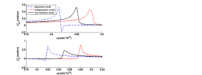
The variation of ks​I∓k_{sI}^{\mp} according to the frequency can be shown by the dispersion relation diagram. It is depicted in figure 2.
Refer to caption
Figure 2: Symmetric and antisymmetric SPP modes dispersion relation. (a) real part and (b) imaginary part of the wave number. Where d=60 nm, the dielectric media with n=1.9726−i​0.081n=1.9726-i0.081 and the metal film with ωp=14.02×10¹⁵\omega_{p}=14.02\times 10^{15}(Rad/s) and γ=6.25×10¹³\gamma=6.25\times 10^{13}(Rad/s) have been considered. (The data are in [22]).

In Fig. 2 despite of different behavior for symmetric and antisymmetric modes, there is a same prediction.
In general, in the frequency ranges that in the loss case ks​I∓k_{sI}^{\mp} is negative, the SPP modes can be amplified otherwise they are attenuated.
Moreover, it can be shown that for thick film the dispersion relation of symmetric and antisymmetric modes are identical and are in accordance with the one interface SPP mode [23].

IV.3 Studying the influence of the dielectric media on the SPP modes

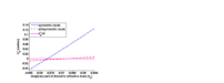
Besides the frequency, the different gain media (dielectric media) can affect the SPP modes behavior. This is illustrated schematically in Fig. 3.
Refer to caption
Figure 3: Variation of ks​Ik_{sI} of the SPP modes in the vicinity of different gain media. where nd=1.9726n_{d}=1.9726 and ω=4.8×10¹⁵​R​a​d/s\omega=4.8\times 10^{15}Rad/s.

Fig.3 shows some interesting points: first, any gain media adjusted to the metal thin film can not amplify the SPP modes. Indeed, for amplifying kdk_{d} and ks​I∓k^{\mp}_{sI} must be negative simultaneously. Second, for a particular kdk_{d} the operation of the system is different for symmetric and antisymmetric modes. This is discussed in more detail later. Third, the slope of the lines indicates that for a given kdk_{d} range, the variation of the symmetric mode in comparison with ks​I∓=0k^{\mp}_{sI}=0 (no gain and no loss) is very greater than the antisymmetric mode. Fourth, except of very small range of kdk_{d} (very close to the ks​I∓=0k^{\mp}_{sI}=0 for symmetric mode) the rate of amplifying or attenuating symmetric mode is very faster than the antisymmetric mode.
In order of illustration and comparison the variation of SPP modes in these ranges, we plot the magnetic field average Eq. (36) for coherent symmetric and antisymmetric modes for different ranges of kdk_{d} .

IV.3.1 Investigating the variation of coherent SPP modes under different gain media

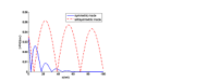
According to Fig.3, for different ranges of kdk_{d} the SPP modes suffer different conditions. The first condition is where two SPP modes are attenuated. For instance, by considering the dielectric media with n=0.9726−i​0.063n=0.9726-i0.063 the ks​I∓k^{\mp}_{sI} of the SPP modes are positive. It means that the gain of the dielectric media can not compensate the loss of the metal and the SPP modes are also attenuated. It is shown schematically in Fig.4 .
Refer to caption
Figure 4: Attenuation of two modes on the z=0z=0 interface. where |α|2=7|\alpha|^{2}=7, θ=1.5\theta=1.5 Rad. ks​I+=7.8029×10⁷k_{sI}^{+}=7.8029\times 10^{7}(Rad/nm) and ks​I−=2.7617×10⁶k_{sI}^{-}=2.7617\times 10^{6}(Rad/nm) .

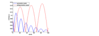
In the second condition, the system’s operation is different for symmetric and antisymmetric modes. For example, the dielectric media with n=0.9726−i​0.072n=0.9726-i0.072 cause the system attenuates the symmetric mode but amplifies the antisymmetric mode. It is shown in Fig.5.
Refer to caption
Figure 5: Attenuation of symmetric modeks​I+=2.5858×10⁷k_{sI}^{+}=2.5858\times 10^{7}(Rad/nm) and amplification of antisymmetric modeks​I−=−1.96×10⁶k_{sI}^{-}=-1.96\times 10^{6} (Rad/nm) on the z=0z=0 interface.

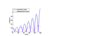
The amplification of symmetric and antisymmetric modes simultaneously is occurred in the third condition where for a given kdk_{d}, the ks​I∓k^{\mp}_{sI} is negative for two modes. Fig. 6 shows this condition where the refractive index of dielectric media is n=0.9726−i​0.08n=0.9726-i0.08. It means that for the two modes the gain of the dielectric media is sufficient to overcome the loss of the metal.
Refer to caption
Figure 6: Amplification of two modes on the z=0z=0 interface. where ks​I+=−1.8673×10⁷k_{sI}^{+}=-1.8673\times 10^{7}(Rad/nm) and ks​I−=−6.1217×10⁶k_{sI}^{-}=-6.1217\times 10^{6} (Rad/nm).

As the Fig.3 illustrates except the small range of kdk_{d},the magnitude of ks​I+k_{sI}^{+} is greater than ks​I−k_{sI}^{-}, therefore for a special condition the rate of variation for symmetric mode is noticeable than the antisymetric mode, as Figs.(4-6) demonstrate obviously. Moreover by comparison the Figs.(4-6), one can find that for different conditions, the changing of symmetric mode behavior is more noticeable than another.
A very interesting point is that, only for one magnitude of kdk_{d}, the behavior of two modes is the same. It is the point of intersection of two graphs in Fig.3. Fig.7 shows this condition where the optical property of dielectric media is n=0.9726−i​0.07747n=0.9726-i0.07747.

Refer to caption
Figure 7: The same behavior of two modes on the z=0z=0 interface. where ks​I+=ks​I−=−4.81×10⁶k_{sI}^{+}=k_{sI}^{-}=-4.81\times 10^{6}(Rad/nm) .

Moreover, the same figures are obtained for the modes that propagate along the z=dz=d interface.

IV.3.2 Comparison between coherent and squeezed SPP modes state

By applying Eqs.(37) and (38) into the Eq.(36), the average of magnetic field is obtained for coherent and squeezed SPP state. For more investigation, we consider α=|α|​ei​θ\alpha=|\alpha|e^{i\theta} as a complex number. The influence of the phase θ\theta on the average of the SPP magnetic filed for one interface system is studied in [11]. Such result is obtained for two interfaces system which shows that the difference between coherent and squeezed state is significant for θ=1.5\theta=1.5. In Fig.8, the difference between the magnetic field average for coherent and squeezed states that propagate in the amplifying system is illustrated.
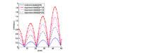
Refer to caption
Figure 8: The difference between the average of the symmetric mode’s magnetic field. where n=0.9726−i​0.08n=0.9726-i0.08 is chosen for dielectric media.

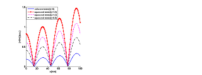
The average of magnetic field for antisymmetric mode is shown in Fig.9.
Refer to caption
Figure 9: The difference between the average of the antisymmetric mode’s magnetic field.

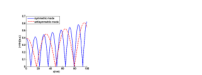
From Figs. 8 and 9 one can deduce that the drastic difference is occurred between squeezed and coherent states. It can be generalized to other amplifying or attenuating system.

V conclusion

In this paper we have provided another approach for quantization of SPP modes on the thin film structure, based on Green’s tensor method which contains some new quantum concepts in the SPP field such as noise current, field fluctuations, and Langevin equations. Moreover, this approach enable us to study the influence of the different conditions on the propagation of the SPP modes. The results are classified as follows:
First, for certain media, the variation of frequency can cause SPP modes amplification or attenuation. It also has been shown that the behavior of symmetric and antisymmetric modes is different in frequency domain.
Second, for certain frequency, the amplifying or attenuating SPP modes is dependent on the optical parameter of the dielectric media adjusted to the metal film. We have also compared the behavior of two SPP modes with each other for different media.
Third, we have illustrated that the drastic difference is between different types of SPP modes, i. e., coherent and squeezed states.

appendix A

In order to prove the Eq.(29), it is neccesary to derive some relations:

[A^(r,t),−ϵ0E^(r′,t)]=∫0∞dω|D|2μ02iωϵ0β′(ω)2​π​ks​I∓×\displaystyle[\hat{A}(r,t),-\epsilon_{0}\hat{E}(r^{{}^{\prime}},t)]=\int_{0}^{\infty}\text{d}\omega|D|^{2}\mu_{0}^{2}\dfrac{i\omega\epsilon_{0}\beta^{{}^{\prime}}(\omega)}{2\pi k^{\mp}_{sI}}\times
|ks∓|2ks​R∓{eiks∓|x−x′|ks∓+e−iks∗⁣∓|x−x′|ks∗⁣∓}×\displaystyle\dfrac{|k_{s}^{\mp}|^{2}}{k^{\mp}_{sR}}\{\dfrac{e^{ik_{s}^{\mp}|x-x^{{}^{\prime}}|}}{k_{s}^{\mp}}+\dfrac{e^{-ik_{s}^{{*\mp}}|x-x^{{}^{\prime}}|}}{k^{*\mp}_{s}}\}\times
{(x^−iks∓ν0z^)eν0​zΘ(−z)∓(x^+iks∓ν0z^)e−ν0​(z−d)Θ(z−d)+\displaystyle\{(\hat{x}-i\dfrac{k_{s}^{\mp}}{\nu_{0}}\hat{z})e^{\nu_{0}z}\Theta(-z)\mp(\hat{x}+i\dfrac{k_{s}^{\mp}}{\nu_{0}}\hat{z})e^{-\nu_{0}(z-d)}\Theta(z-d)+
A[(x^+iks∓νmz^)e−νm​z∓(x^−iks∓νmz^)eνm​(z−d)]Θ(z)Θ(d−z)}×\displaystyle A[(\hat{x}+i\dfrac{k_{s}^{\mp}}{\nu_{m}}\hat{z})e^{-\nu_{m}z}\mp(\hat{x}-i\dfrac{k_{s}^{\mp}}{\nu_{m}}\hat{z})e^{\nu_{m}(z-d)}]\Theta(z)\Theta(d-z)\}\times
{(x^+iks∗⁣∓ν0∗z^)eν∗0z′Θ(−z′)∓(x^−iks∗⁣∓ν0∗z^)e−ν∗0(z′−d)Θ(z′−d)+\displaystyle\{(\hat{x}+i\dfrac{k_{s}^{{*\mp}}}{\nu^{*}_{0}}\hat{z})e^{\nu^{*}_{0}z^{{}^{\prime}}}\Theta(-z^{{}^{\prime}})\mp(\hat{x}-i\dfrac{k_{s}^{{*\mp}}}{\nu^{*}_{0}}\hat{z})e^{-\nu^{*}_{0}(z^{{}^{\prime}}-d)}\Theta(z^{{}^{\prime}}-d)+
A∗[(x^−iks∗⁣∓νm∗z^)e−ν∗mz′∓(x^+iks∗⁣∓νm∗z^)eν∗m(z′−d)]Θ(z′)Θ(d−z′)}.\displaystyle A^{*}[(\hat{x}-i\dfrac{k_{s}^{{*\mp}}}{\nu^{*}_{m}}\hat{z})e^{-\nu^{*}_{m}z^{{}^{\prime}}}\mp(\hat{x}+i\dfrac{k_{s}^{{*\mp}}}{\nu^{*}_{m}}\hat{z})e^{\nu^{*}_{m}(z^{{}^{\prime}}-d)}]\Theta(z^{{}^{\prime}})\Theta(d-z^{{}^{\prime}})\}. (39)

On the other hand, the Green’s tensor for a dielectric-metal- dielectric structure (see Eq.(20)) satisfy the following relation:

∫dsImϵ(s,ω)G(r,s,ω)⋅G∗(s,r′,ω)=\displaystyle\int\text{d}s\text{Im}\epsilon(s,\omega)G(r,s,\omega)\cdot G^{*}(s,r^{{}^{\prime}},\omega)=
|ks∓|22​ks​R∓​ks​I∓γ′(ω)|D|2{eiks∓|x−x′|ks∓+e−ik∗⁣∓s|x−x′|ks∗⁣∓}×\displaystyle\dfrac{|k_{s}^{\mp}|^{2}}{2k^{\mp}_{sR}k^{\mp}_{sI}}\gamma^{{}^{\prime}}(\omega)|D|^{2}\{\dfrac{e^{ik_{s}^{\mp}|x-x^{{}^{\prime}}|}}{k_{s}^{\mp}}+\dfrac{e^{-ik^{*\mp}_{s}|x-x^{{}^{\prime}}|}}{k^{*\mp}_{s}}\}\times
{(x^−iks∓ν0z^)eν0​zΘ(−z)∓(x^+iks∓ν0z^)e−ν0​(z−d)Θ(z−d)+\displaystyle\{(\hat{x}-i\dfrac{k_{s}^{\mp}}{\nu_{0}}\hat{z})e^{\nu_{0}z}\Theta(-z)\mp(\hat{x}+i\dfrac{k_{s}^{\mp}}{\nu_{0}}\hat{z})e^{-\nu_{0}(z-d)}\Theta(z-d)+
A[(x^+iks∓νmz^)e−νm​z∓(x^−iks∓νmz^)eνm​(z−d)]Θ(z)Θ(d−z)}×\displaystyle A[(\hat{x}+i\dfrac{k_{s}^{\mp}}{\nu_{m}}\hat{z})e^{-\nu_{m}z}\mp(\hat{x}-i\dfrac{k_{s}^{\mp}}{\nu_{m}}\hat{z})e^{\nu_{m}(z-d)}]\Theta(z)\Theta(d-z)\}\times
{(x^+iks∗⁣∓ν0∗z^)eν∗0z′Θ(−z′)∓(x^−iks∗⁣∓ν0∗z^)e−ν∗0(z′−d)Θ(z′−d)+\displaystyle\{(\hat{x}+i\dfrac{k_{s}^{{*\mp}}}{\nu^{*}_{0}}\hat{z})e^{\nu^{*}_{0}z^{{}^{\prime}}}\Theta(-z^{{}^{\prime}})\mp(\hat{x}-i\dfrac{k_{s}^{{*\mp}}}{\nu^{*}_{0}}\hat{z})e^{-\nu^{*}_{0}(z^{{}^{\prime}}-d)}\Theta(z^{{}^{\prime}}-d)+
A∗[(x^−iks∗⁣∓νm∗z^)e−ν∗mz′∓(x^+iks∗⁣∓νm∗z^)eν∗m(z′−d)]Θ(z′)Θ(d−z′)},\displaystyle A^{*}[(\hat{x}-i\dfrac{k_{s}^{{*\mp}}}{\nu^{*}_{m}}\hat{z})e^{-\nu^{*}_{m}z^{{}^{\prime}}}\mp(\hat{x}+i\dfrac{k_{s}^{{*\mp}}}{\nu^{*}_{m}}\hat{z})e^{\nu^{*}_{m}(z^{{}^{\prime}}-d)}]\Theta(z^{{}^{\prime}})\Theta(d-z^{{}^{\prime}})\}, (40)

here

γ′(ω)=\displaystyle\gamma^{{}^{\prime}}(\omega)= Im​ϵm​(1+|ks∓|2|ν0|2)​2ν0+ν0∗+\displaystyle\text{Im}\epsilon_{m}(1+\dfrac{|k_{s}^{\mp}|^{2}}{|\nu_{0}|^{2}})\dfrac{2}{\nu_{0}+\nu_{0}^{*}}+
Imϵd|A|2×{(1+|ks∓|2|νm|2)2​(1−e−(νm+νm∗)​d)νm+νm∗\displaystyle\text{Im}\epsilon_{d}|A|^{2}\times\{(1+\dfrac{|k_{s}^{\mp}|^{2}}{|\nu_{m}|^{2}})\dfrac{2(1-e^{-(\nu_{m}+\nu_{m}^{*})d})}{\nu_{m}+\nu_{m}^{*}}
∓(1−|ks∓|2|νm|2)2​(e−νm∗​d−e−νm​d)νm−νm∗}.\displaystyle\mp(1-\dfrac{|k_{s}^{\mp}|^{2}}{|\nu_{m}|^{2}})\dfrac{2(e^{-\nu_{m}^{*}d}-e^{-\nu_{m}d})}{\nu_{m}-\nu_{m}^{*}}\}. (41)

and ϵ⁡(s,ω)\epsilon(s,\omega) has been given in Eq.(12). By rewritting Eq.(39) according to Eq.(40) and considering the general property of Green’s tensor[29]

∫dsImϵ(s,ω)G(r,s,ω)⋅G∗(s,r′,ω)=c2ω2ImG(r,r′,ω)\int\text{d}s\text{Im}\epsilon(s,\omega)G(r,s,\omega)\cdot G^{*}(s,r^{{}^{\prime}},\omega)=\dfrac{c^{2}}{\omega^{2}}\text{Im}G(r,r^{{}^{\prime}},\omega) (42)

The desired equation can be deduced:

[A^(r,t),−ϵ0E^(r′,t)]=∫dωiωϵ0μ02β′(ω)πγ′(ω)c2ω2ImG(r,r′,ω).\displaystyle[\hat{A}(r,t),-\epsilon_{0}\hat{E}(r^{{}^{\prime}},t)]=\int\text{d}\omega\dfrac{i\omega\epsilon_{0}\mu_{0}^{2}\beta^{{}^{\prime}}(\omega)}{\pi\gamma^{{}^{\prime}}(\omega)}\dfrac{c^{2}}{\omega^{2}}\text{Im}G(r,r^{{}^{\prime}},\omega).

References

  • [1] S. A. maier, Plasmonics: Fundamentals and Applications (Springer, Vew York, 2007).
  • [2] T. Zhang and F. Shan. “Development and application of surface plasmon polaritons on optical amplification.” Journal of Nanomaterials 2014 495381 (2014).
  • [3] E. Altewischer, M. P. Van Exter, J. P. Woerdman, “Plasmon assisted transmission of entangled photons.” Nature, 418, 304 (2002).
  • [4] E. Moreno, F. J. Garcia Vidal, D Erni, …“Theory of plasmon assisted transmission of entangled photons.” Phys. Rev. Lett, 92 236801(2004).
  • [5] A. Huck, S. Smolka, P. Lodahl, …“Demonstration of quadrature squeezed surface plasmons in a gold waveguide.” Phys. Rev. Lett, 102 246802(2009).
  • [6] Y. LiHua, W. YongGang and Y. Bojun,“Description of squeezed surface plasmons.” Sci China Phys. Mech. Astorn., 541583(2011)
  • [7] J. L. Van Velsen, J. Tworzyldo and C. W. J. Beenakker, “Scattering theory of plasmon-assisted entanglement transfer and distillation.” Phys. Rev. A, 68 043807 (2003).
  • [8] D. E. Chang, A. S. Sørensen, P. R. Hemmer and M. D. Lukin,“Quantum Optics with Surface Plasmons.” Phys. Rev. Lett., 97 053002 (2006).
  • [9] D. E. Chang, A. S. Sørensen, E. A. Demler and M. D. Lukin,“A single photon transistor using nanoscale surface plasmons.” Nature Phys., 3 807 (2007).
  • [10] J. M. Elson and Ritchie,“Photon Interactions at a Rough Metal Surface.” Phys. Rev. B, 4 4129 (1971).
  • [11] Z. Allameh, R. Roknizadeh and R. Masoudi. “Quantization of surface plasmon polariton by Green’s tensor method in amplifying and attenuating media.” submitted, arXiv:1505.00677 (2015).
  • [12] T. Söndergaard and B. Tromborg, “General theory for spontaneous emission in active dielectric microstructures: Example of a fiber amplifier.” Phys. Rev. A 64 033812 (2001).
  • [13] T. Söndergaard and S. I. Bozhevolnyi,“Surface plasmon polariton scattering by a small particle placed near a metal surface: An analytical study.” Phys. Rev. B 69 045422 (2004).
  • [14] J. Jung and T. Söndergaard, “Green’s function surface integral equation method for theoretical analysis of scatterers close to a metal interface.” Phys. Rev. B 77 245310 (2008).
  • [15] V. Siahpoush, T. Söndergaard and J. Jung,“Green’s function approach to investigate the excitation of surface plasmon polaritons in a nanometer-thin metal film.” Phys. Rev. B 85 075305 (2012).
  • [16] R. Matloob, R. Loudon, S. M. Barnett and J. Jeffers,“Electromagnetic field quantization in absorbing dielectrics” Phys. Rev. A 52 4823,(1995).
  • [17] T. Gruner and D.-G. Welsch,“Green-function approach to the radiation-field quantization for homogeneous and inhomogeneous Kramers-Kronig dielectrics.” Phys. Rev. A 53 1818 (1996)
  • [18] L. Knöll, S. Scheel, D.-G. Welsch, QED in dispersing and absorbing media:Coherence and Statistics of Photons and Atoms edited by J. Perina (John Wiley & Son, New York, 2001).
  • [19] A. Tip, L. Knöll, S. Scheel, and D.-G. Welsch,“On the equivalence of the Langevin and auxiliary field quantization methods for absorbing dielectrics.” Phys. Rev. A 63 043806 (2001).
  • [20] H. T. Dung, L. Knöll and D.-G. Welsch,“Three-dimensional quantization of the electromagnetic field in dispersive and absorbing inhomogeneous dielectrics.” Phys. Rev. A 57 3931 (1998).
  • [21] R. Kubo, “The fluctuation-dissipation theorem.” Rep. Prog. Phys. 29 255 (1966) .
  • [22] D. Ballester, M. S. Tame, C. Lee, J. Lee and M. S. Kim,“Long-range surface plasmon polariton excitation at the quantum level.” Phys. Rev. A79 053845 (2009).
  • [23] D. Genov, M. Ambati and X. Zhang, “Surface plasmon amplification in planar metal films.” Quantum Electronics, IEEE. 43 1104 (2007).
  • [24] I. Suarez, E. P. Fitrakis, P. Rodriguez-Canto, R. Abargues, I. Tomkos and J. Martinez-Pastor, (2012, July). “Surface plasmon-polariton amplifiers.” In Transparent Optical Networks (ICTON), 2012 14th International Conference on (pp. 1-5). IEEE.
  • [25] M. A. Noginov, V. A. Podolskiy, G. Zhu, M. Mayy, M. Bahoura, J. A. Adegoke, B. A. Ritzo, and K. Reynolds. “Compensation of loss in propagating surface plasmon polariton by gain in adjacent dielectric medium.” Optics express 16 1385 (2008).
  • [26] M. A. Noginov, G. Zhu, M. Bahoura, J. Adegoke, C. E. Small, B. A. Ritzo, V. P. Drachev, and V. M. Shalaev. “Enhancement of surface plasmons in an Ag aggregate by optical gain in a dielectric medium.” Optics letters. 31 3022 (2006).
  • [27] P. Berini, and I. De Leon. “Surface plasmon-polariton amplifiers and lasers.” Nature Photonics. 6 16 (2012).
  • [28] I. Avrutsky. “Surface plasmons at nanoscale relief gratings between a metal and a dielectric medium with optical gain.” Phys. Rev. B 70, 155416 (2004).
  • [29] S. Y. Buhmann, Dispersion Force I (Springer, Berlin, 2012).