The role of the parton distribution functions in QCD theory is essential to describe both unpolarized and polarized reactions, so a tremendous effort has been undertaken to find the most accurate distributions. In the litterature we remark that unpolarized and polarized PDF are treated as separated entities [1]-[9], however, a simultaneous treatment of unpolarized and polarized PDF should in principle gives a more constrained determination. Since many years we have adopted this point of view in the framework of a statistical model where the PDF are built in from their helicity components.[10, 11]

In the absence of a theory for the parton distributions two approaches are currently proposed. In one approach the distributions are approximated by different polynomials which require numerous parameters, with such an hypercube a carefull numerical analysis of the errors is necessary in order to get the most precise values of the distributions, however no attention is paid to the physical structure of the partons nor on the meaning of the parameters values. In our approach the physical structure of the distributions is introduced through a statistical model, this information allows us to work with a reduce number of parameters (21) whose meaning can be justified. In both case a good description of the experimental data is obtained so we have a possible choice between a numerical formulation of the distributions versus a physical one where more emphasize is put on the partons structure [12].

The application of a statistical model, for instance, to a proton at rest which contains three quarks seems not justified due to the low number of elements. But when accelerated in a collider the energy increase has not only an effect on its mass but also to create a large number of $q~\bar{q}$ pairs or a quark gluon plasma which in a p-p collison materialize mainly in primary unstable particles observed in a detector as large number of tracks. These occurence of numerous pairs provide a justification for a statistical treatment of the partons interaction process.

Let us mention an other application of the statistical model to different elastic scattering reactions in terms of quarks PDF defined in impact parameter space, we have shown, in particular, that the gluon contribution is essential to explain the dip structure of the pp elastic differential cross section [13].

The paper is organized a follow: in section 2, the role of the thermodynamical potentials is discussed, in section 3 we consider the entropy of quarks states and show that the parameters values obtained from a fit correspond to a maximum entropy of these states. The same property is derived for the structure functions $F^{2}_{p}$ and $g^{1}_{p}$, and also for the quarks. In section 4 an analysis of the polarized gluon leads to define a neural model for its structure and in section 5 we developp an extension of this model to quarks.

In the statistical model the thermodynamical helicity dependent potentials $X^{\pm}$ play an essential role in the construction of the polarized quark distributions and so have a direct consequence on the behavior of the polarized structure functions. The helicity decomposition of the quarks PDF is given by a quasi Fermi-Dirac distribution which is defined at the input scale $Q^{2}=1$GeV² by the expressions:

$$xq^{\pm}(x)=\frac{A_{q}X_{q}^{\pm}x^{b_{q}}}{\exp[(x-X_{q}^{\pm})/\bar{x}]+1}+\frac{\tilde{A}_{q}x^{\tilde{b}_{q}}}{\exp(x/\bar{x})+1}\,,$$

(1)

$$x\bar{q}^{\pm}(x)=\frac{\bar{A}_{q}}{X_{q}^{\mp}}\cdot\frac{x^{\bar{b}_{q}}}{\exp[(x+X_{q}^{\mp})/\bar{x}]+1}+\frac{\tilde{A}_{q}x^{\tilde{b}_{q}}}{\exp(x/\bar{x})+1}\,.$$

(2)

The last term is a diffractive contribution whose effect is to enhance the values of the unpolarized quarks at low $x$. The polarized quarks are defined by the difference $x\Delta q(x)=xq^{+}(x)-xq^{-}(x)$ and the unpolarized one by the sum $xq(x)=xq^{+}(x)+xq^{-}(x)$, the antiquarks $\bar{q}$ have a similar definition. In these expressions $\bar{x}$ is a universal temperature, the introduction of the potential $X^{\pm}$ and $(X^{\pm})^{-1}$ in front of Eqs. (1-2) comes from the relation between the Transverse Momentum Distribution and the PDF [14]. In a recent fit of unpolarized and polarised data made in Ref. [12] we have obtained for the $u,d,s$ potentials, ²² 2 The PDF are evolved with the HOPPET program [15]. See Ref. [12] for more details. A Fortran program to compute the PDF independently of HOPPET is available upon request.

	$\displaystyle X_{u}^{+}=0.475\pm 0.0008,\quad X_{u}^{-}=0.307\pm 0.001,\quad X_{d}^{+}=0.245\pm 0.001,$
	$\displaystyle X_{d}^{-}=0.309\pm 0.001,\quad X_{s}^{+}=0.011\pm 0.0008,\quad X_{s}^{-}=0.015\pm 0.001\,.$		(3)

From these values we obtain the potentials hierarchy

$$X_{s}^{+}<X_{s}^{-}<X_{d}^{+}<X_{u}^{-}<X_{d}^{-}<X_{u}^{+}\,,$$

(4)

which is responsible of the quarks order of magnitude. Notice that the $u$ and the $d$ potentials are relatively stable since the analysis made in 2002 [10], it means that their values are a real intrinsic property of quarks, and they represent the master parameters of the statistical model.

In Fig. 1 a plot of the polarized light quarks at $Q^{2}=4\mbox{GeV}^{2}$ is shown with their corresponding maximum potentials, we observe a correlation between the potentials values and the maximum or the minimum of the PDF. From Eq. (1) the sign of the polarized PDF $\Delta q=q^{+}-q^{-}$ is related to the value of the thermodynamical potential helicity, more precisely, on the relative values of the potentials $X^{+}$ and $X^{-}$, the equality being excluded because it leads to a vanishing polarized PDF at the input scale, so we are led with two possibilities $X^{-}>X^{+}$ and $X^{-}<X^{+}$. In the case of $u$ quark $X_{u}^{-}<X_{u}^{+}$ so $\Delta u$ is positive, while for the $d$ quark $X_{d}^{-}>X_{d}^{+}$ so $\Delta d$ is negative, and for the strange quark $s$ we have $X_{s}^{-}>X_{s}^{+}$ leading also to a negative $\Delta s$ (see HERMES experiment [16]).

For the antiquarks, the chiral structure of QCD gives an important property which allow to relate quark and antiquark distributions. The potential of an antiquark $\bar{q}_{i}^{~-h}$ of helicity -h is opposite to the potential of a quark $q_{i}^{h}$ of helicity h

$$X_{0\bar{q}}^{-h}=-X_{0q}^{h}\,.$$

(5)

So in the expression given by Eq. (2) the thermodynamical potentials have been interchanged with respect to the helicity $\pm$ and their sign taken to be opposite. This change of sign is due to the fact that a $q~\bar{q}$ pair can be created by a gluon through the process $g\rightarrow q+\bar{q}$. Due to the interchange of the potentials the sign of $\Delta\bar{u}$ is positive while $\Delta\bar{d}$, $\Delta\bar{s}$ keep their negative sign. The respective signs are confirmed by the parity violating asymmetry $A_{L}^{PV}$ measured by the STAR polarized experiment [17] in the process $\overrightarrow{p}p\rightarrow W^{\pm}+X$.

Taking into account the numerical value of the potentials how they influence the spin structure functions, we will give two exemples. The polarized structure function $xg_{1}^{p}$ has a maximum around $x=0.4$, see Fig. 2, now we know that $\Delta u$ which gives the major contribution has a thermodynamical potential $X_{0u}^{+}=0.46$, so we observe a correspondance between this potential and the maximum in $xg_{1}^{p}$. An other exemple is given by $xg_{1}^{n}$, the data show that $g_{1}^{n}$ is mainly negative over a large $x$ region this fact can be explained by the inequality of the thermodynamical potentials $X_{0d}^{+}<X_{0d}^{-}$ which implies $\Delta(d^{+}-d^{-})<0$, we also see in the figure that around $x=0.45$ it has a postive maximum which reflects the influence of the $u^{+}$ contribution at large $x$ compared to $\Delta d$ which is depressed in this region.

In the previous section we have focused on the polarized PDF, the unpolarized ones are obtained from the relation $q=q^{+}+q^{-}$, we show in Fig. 3 the unpolarized PDF at $Q^{2}=10\mbox{GeV}^{2}$. With the parameters defined above they give a good description of the unpolarized structure functions in deep inelastic scattering, the neutrino cross sections, the neutral and charged current cross sections, and the jets production up to LHC energy, see Ref. [12].

We will explore a new property of the unpolarized PDF by considering a physical quantity precisely the entropy. The entropy can be calculated according to the definition given in Ref. [29] Eq. (16)

$$E(Q^{2},x)=-\sum_{i}\left[xq_{i}(Q^{2},x)\ln{(xq_{i}(Q^{2},x))}+(1-xq_{i}(Q^{2},x))\ln{(1-xq_{i}(Q^{2},x))}\right]\,,$$

(6)

where the sum runs over the quark components. We first remark that the vanishing of $xq_{i}(Q^{2},x)$ for $x=1$, implies that $E(Q^{2},x)=0$ in this limit. We propose to compute the entropy for the states made with $|2u+d>$, $|u+d+s>$ and $|2\bar{u}+\bar{d}>$, at a fixed $Q^{2}=10\mbox{GeV}^{2}$ as a function of $x$. In Fig. 4 we see that the first state is largely dominant over the last ones which seems to reflect the importance of matter over anti-matter.

The curves shown in Figure 4 have been calculated with the values of the potentials obtained from a fit of experimental data discussed above, then a question arises, what is the origin of these values, does exist a possibility to obtain them independently of experimental data? In the PDF formulas described above we have introduced the following parameters: a normalization $A$, a power $b$ of the variable $x$, a temperature $\bar{x}$ and the potentials. For a matter of simplification in the calculation let us assume that the following parameters $A,~b,~\bar{x}$ are held fixed to their actual values and consider now the potentials as free parameters which will be determined from a calculation of the optimal value of the entropy (6) for a given value of $x$ and $Q^{2}$. In complete generality all the the parameters of the model should have been considered as free, but due the complexity of the computation we restrict our search only to the six potentials defined as the master parameters of the model.

For this purpose we consider $E(Q^{2},x)$ given by Eq. (6) as an objective function which depends on $u$, $d$, $s$ quarks subjects to the constraints

	$\displaystyle 0<X_{0q}^{h}<1,\quad\quad\int u_{v}(x)dx=2,\quad\quad\int d_{v}(x)dx=1,$
	$\displaystyle\Delta u(x)\geq 0,\quad\quad\Delta d(x)\leq 0,\quad\quad\Delta s(x)\leq 0,$
	$\displaystyle\int(xu(x)+xd(x)+xs(x))dx\leq 1,\quad\quad\int(s(x)-\bar{s}(x))dx=0\,.$		(7)

The goal is to solve the sytem of equations (6)-(7) with respect to the thermodynalical potentials (supposed to be unknown) associated with $u$, $d$ and $s$. The optimization is performed with the NLOPT software [30], which involves the objective function, the constraints and their gradients with respect to the parameters. In addition, to confirm the results a brute-force method is also applied, it consists to find the maximum of the entropy by varying the parameters in a range defined as $\pm 50\%$ of the fitted parameters values.

We consider for a fixed $Q^{2}=10\mbox{GeV}^{2}$ a set of 20 $x$ values in the range $10^{-3}<x<1$, the solutions for the optimal entropy are shown in Fig. 4 as circles for the state $|2u+d>$, and squares for the state $|u+d+s>$, one observes that their values are close to the solids curves. These results show that the parameters obtained by this method have the same values (with an error around 2%) as the original ones obtained from a fit, so the entropy obtained from experimental data satisfies an optimal principle.

We can envisage also to compute the entropy of a polarized state $|2\Delta u+\Delta d>$, in this case there is a the difficulty which comes from the fact that to polarize, for instance, a proton one needs to apply a strong magnetic field, so there is coupling between the proton and an external field which introduces a complicated situation for the computation of the entropy because one has to disantangle the contribution coming from the external field and the other from the state itself.

Nevertheless, we show in Fig. 4 the resulting entropy with a dash-dotted curve, the values are much smaller than in the case of an unpolarized proton where the situation is more clear because the proton can be considered as in a free state. As a conclusion the calculation of the entropy obtained in an independent way from experiment has the consequence that the quarks PDF obtained from a fit correspond to a maximum entropy principle, so the structure functions must share in some way the same property. We know that the entropy is sometimes associated with the disorder of a system and increases with energy. In Fig. 5 the difference of the entropy $\delta E$ between $Q^{2}=1~\mbox{and}~10\mbox{GeV}^{2}$ is effectively growing for the states discussed above. The state which involves the strange quark has the largest effect with respect to the disorder.

A comparison of the optimum calculated entropy with experiment is not easy, an other test can be made with the structure functions. Using the same method as above, we consider again the thermodynamical potentials as free parameters in a certain range of values and search a maximum for the strcture functions $F_{2}^{p}$ and $g_{1}^{p}$ for a fixed $x$ and $Q^{2}$. We find that the maximum is obtained when the potentials values are those obtained in the fit, so the following relation is derived

$$F_{2}^{p}~\mbox{maximum}=F_{2}^{p}~\mbox{fit}=F_{2}^{p}~\mbox{experimental}\,,$$

(8)

with the same relation for $g_{1}^{p}$.

In the above results the quark distributions are the essential source of information to obtain an optimum a property which should be reflected in the quarks themselves. To prove this we consider that in the unpolarized up and down quarks the potentials are now free parameters and a search is made for a maximum value given a fixed $Q^{2}=10\mbox{GeV}^{2}$ and $x=0.15$. In Fig. 6 we plot the u and d values as a function of $X^{+}$ and $X^{-}$ limited to a certain domain which generates a surface. Now, if we look for a maximum by imposing the constraints Eqs . 7 we obtain as a solution only one couple $X^{+},X^{-}$ with a $u$ and $d$ values which correspond to those obtained in the fit (red point in the figure). The same result is also obtained for the polarized $\Delta u$ and $\Delta d$. So the optimum obtained for the entropy and the structure functions find its origin on the quarks properties. Let us mention that this maximum values of the light quarks unpolarized distriutions is also found with the parametrization MSTW 2008 [31] and CT14 ³³ 3 I thank J. Pumplin for informations on CT14 PDFs. [32].

From this result we infer that nature tends to produce observable quantities with a maximum probability taking into account some physical constraints, it remains to explain the origin of this effect.

The polarized gluon distribution is today not well known and subject to a large debate concerning its expression and sign. Our purpose is to clarify the choice made in our original model at the input scale and to propose a new interpretation in the context of a neural structure. In the statistical model it is natural to assume a quasi Bose-Einstein distribution for both $G$ and $\Delta G$, so we define for the gluon at the input scale $Q_{0}^{2}=1\mbox{Gev}^{2}$

$$xG(x,Q^{2}_{0})=\frac{A_{G}x^{b_{G}}}{\exp(x/\bar{x})-1}\,,$$

(9)

and for the polarized distribution

$$x\Delta G(x,Q^{2}_{0})=\tilde{A}_{G}x^{\tilde{b}_{G}}P(x)\cdot\frac{1}{\exp(x/\bar{x}-1)}\,,$$

(10)

where for $P(x)$ we made the choice [33]

$$P(x)=\frac{1}{(1+c_{G}x^{d_{G}})}\,,$$

(11)

notice that the introduction of an analogous rational multiplicative factor is also used in Ref. [34]. A fit of polarized DIS data gives the values [12]

	$\displaystyle A_{G}=36.778\pm 0.085,~b_{G}=1.020\pm 0.0014,~\tilde{A}_{G}=26.887\pm 0.050,$
	$\displaystyle\tilde{b}_{G}=0.163\pm 0.005,~c_{G}=0.006\pm 0.0005,~d_{G}=-6.072\pm 0.350\,,$		(12)

and for the temperature $\bar{x}=0.090\pm 0.002$. We obtain a $\chi^{2}/d.o.f.=319/269$.

With these parameters $\Delta G(x)$ is positive a property confirmed by experimental data from Hermes [35], Compass [36] and $A^{jet}_{LL}$ from the STAR Collaboration at BNL-RHIC [37]. In our analysis we take advantage that both the unpolarized and polarized gluon are determined in the same fit. We remark that unpolarized quarks and gluon are related through the evolution equations, in the same way the polarized quarks and gluon are related by an other set of evolution equations, now by construction unpolarized and polarized quarks are related because the building blocks are the helicity components, as a consequence all the partons are linked together.

A plot in Fig. 7 of the polarized gluon (dotted curve) at $Q^{2}=2$GeV² shows a maximum in the region $x=0.3$, now from the values of $G(x)$ and $\Delta G(x)$ we can deduce the helicity components (solid and dashed curves) their main difference is located in the same $x$ region.

A priori, it was natural to use for the polarized gluon an analogous expression like Eq. (9) for the gluon which is obtained by setting $c_{G}=0$ in $P(x)$. With this assumption a new fit gives for the parameters

$$\tilde{A}_{G}=(2.46\pm 0.1)10^{-4},~\tilde{b}_{G}=0.294$$

(13)

with a $\chi^{2}/d.o.f.=325/269$, at this level we can consider that the 2 solutions (12)-(13) are equivalent, however, in Fig. 8 we observe a marked difference for $x\Delta G$. The pic obtained at $Q^{2}=4\mbox{GeV}^{2}$ when $c_{G}=0.006$ (solid curve) becomes a flat maximum when $c_{G}=0$ and is reduced by a factor 4 (dashed curve). In order to separate the 2 solutions we refer to the measurement of the double-helicity asymmetry $A_{LL}^{\it jet}$ for $5\leq p_{T}\leq 30\mbox{GeV}$, in the near-forward rapidity region measured recently by the STAR Collaboration [17].

In Fig. 9 we have plotted the solution with $c_{G}\neq 0$ (solid curve)⁴⁴ 4 Results are taken from Ref. [33]. and the solution $c_{G}=0$ (dashed curve). Despite large experimental errors the agreement with data is clearly in favor of $c_{G}\neq 0$ because the other curve grows too slowly with $p_{T}$, so the solution with $c_{G}=0$ is not acceptable.

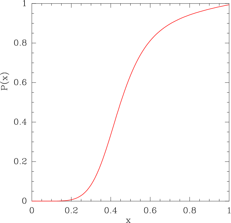
Let us now examine the function $P(x)$ defined by Eq. (11). In Fig 10 a plot versus $x$ at the input scale shows that $P(x)$ is increasing with $x$, its first derivative is maximum for $x=0.41$ and the second derivative (curvature) vanishes at the same $x$ value. The shape of curve and the above properties show a close similarity with a sigmoïd or logistic function whose basic expression is

$$S_{o}(x)=\frac{1}{1+e^{-\lambda x}}\,.$$

(14)

A sigmoïd function is used as an activation function in several domains, in particular, in neural networks applied to structure functions [6, 7], also in the exploration of opacity in elastic hadron scattering [8]. From our previous remark will consider that the $P(x)$ function can now be replaced by a sigmoïd of the form

$$S(x)=\frac{1}{1+e^{-e_{G}x+h_{G}}}\,,$$

(15)

where the parameter $h_{G}$ defines a translation of the curve in the interval $[0\leq x\leq 1]$, so we define a new $x\Delta G$ at the input scale

$$x\Delta G(x,Q^{2}_{0})=S(x)\frac{\tilde{A^{\prime}}_{G}x^{b_{G}}}{\exp(x/\bar{x})-1}\,.$$

(16)

A fit of polarized data yields the values

$$\tilde{A^{\prime}}_{G}=18.987\pm 1.5,~e_{G}=77.94\pm 3.3,~h_{G}=22.18\pm 2.4\,,$$

(17)

$b_{G}$ is the same as in (9), we obtain a $\chi^{2}/d.o.f.=326/271$ very close to the original solution.

For illustration we show in Fig. 11 the function $S(x)$. calculated with the fitted parameters (17).

It is interesting to compare $x\Delta G$ obtained with $P(x)$ and $c_{G}\neq 0$ with the case of $S(x)$. In Fig. 12 the solution with $P(x)$ corresponds to the dashed curve and with $S(x)$ solid curve, we observe that the latter has a more pronounced peak which decreases with $Q^{2}$ and moves slowly toward smaller $x$ values.

The validity of the new polarized gluon can be tested by computing the asymmetry $A_{LL}^{jet}$, the Fig. 13 shows a good agreement between the two solutions, $P(x),c_{g}\neq 0$ and $S(x)$.

In this section we have explored three possibilities to describe the helicity of the gluon. Starting with the expression Eq. (11) used in [12] which was phenomelogical, now we have shown that a more physical expression given by a sigmoïd Eq. (15) gives also a good desciption of polarized experimental data.

How we can interpret the role of the sigmoïd $S(x)$. When 2 protons collide the gluon receives different fractions of the momentum coming from the quarks which are collected statistically with a Bose-Einstein distribution, next the function $S(x)$ plays the role of an activation function which synthesizes in an output signal $\Delta G$. This mechanism allow us to define a neural representation of the polarized gluon whose schematic view is given in Fig. 14.

From this result it is tempting to apply the same representation to the unpolarized gluon, we now introduce in the gluon distribution an activation function (15). A global fit gives the parameters

$$A_{G}=33.23\pm 1.2,~e_{G}=281.16\pm 6.1,~h_{G}=-1.923\pm 0.01\,.$$

(18)

The resulting $S(x)$ function is plotted in Fig. 15, we observe for $x>10^{-3}$ a value of $S(x)$ around 0.9-1 almost independent of $x$. It implies that the activation function makes no modification on the output distribution G, which can be interpreted by the fact that in order to maintain the confinement of quarks any momentum transfer is allowed, also as stated in the introduction the creation of a maximum of $q\bar{q}$ pairs with increasing energy implies no selection.

In this new approach of the polarized gluon we would like to examine the ratio $\Delta G(x,Q^{2})/G(x,Q^{2})$ discussed in Ref. [33]. In Fig. 16 the ratio is plotted as a function of $x$ for four $Q^{2}$ values, in this range the positivity condition $\Delta G(x)/G(x)\leq 1$ is statisfied, and for a fixed $Q^{2}$ it increases with $x$, near the limit $x=1$ the values are very close to 0.5. At the input scale the Bose-Einstein function cancels in Eqs.(9)-(16) it results that $\Delta G/G(x=1)\rightarrow A^{\prime}_{G}S_{G}(1)/A_{G}S_{\Delta G}(1)$, now taking into account the ratio of the normalization factors we obtain the value 0.57, so the limit of the ratio $\Delta G/G$ is different from 1 as required by the counting sum rule.

In the previous section we have focused on the structure of the gluon in a neural model, now a question arises for the quarks, can they share the same structure? The unpolarized quarks PDF are known with a good precision, and most of the parametrizations agree to produce the same values in $x$ and $Q^{2}$, in the polarized case there are more uncertainties but the observed shapes are more or less indentical, so the neural description we give in the gluon case seems not necessary. Nevertheless, looking at our PDF expressions Eqs. (1, 2) we have the product of a Fermi-Dirac distribution by an helicity dependent funcion $Ax^{B}X^{\pm}$ for quarks and $\bar{A}x^{\bar{B}}/X^{\pm}$ for antiquarks, so we can try to apply the same approach where the incoming momentum is collected now by mean of a Ferm-Dirac distribution and then filtered by an activation function to produce the quark distribution. Our objective is to obtain a coherent neural structure for all the unpolarized and polarized PDF. Several possibilities exist to introduce an activation function, we made the following choice where the original parton expressions for $q,\bar{q}~\mbox{and}~G$ are preserved when $S(x)=1$.

$$xq^{\pm}(x)=S_{q}(x)\frac{A_{q}X_{q}^{\pm}x^{b_{q}}}{\exp[(x-X_{q}^{\pm})/\bar{x}]+1}+\frac{\tilde{A}_{q}x^{\tilde{b}_{q}}}{\exp(x/\bar{x})+1}\,,$$

(19)

$$x\bar{q}^{\pm}(x)=S_{\bar{q}}(x)\frac{\bar{A}_{q}}{X_{q}^{\mp}}\cdot\frac{x^{\bar{b}_{q}}}{\exp[(x+X_{q}^{\mp})/\bar{x}]+1}+\frac{\tilde{A}_{q}x^{\tilde{b}_{q}}}{\exp(x/\bar{x})+1}\,.$$

(20)

$$xG(x,Q^{2}_{0})=S_{G}(x)\frac{A_{G}x^{b_{G}}}{\exp(x/\bar{x})-1}\,,$$

(21)

$$x\Delta G(x,Q^{2}_{0})=S_{\Delta G}(x)\tilde{A}_{G}x^{\tilde{b}_{G}}\cdot\frac{1}{\exp(x/\bar{x}-1)}\,,$$

(22)

with an activation function defined by:

$$S_{i}(x)=\frac{1}{1+e^{-e_{i}x+h_{i}}}\,,$$

(23)

the index $i=q,\bar{q},G,\Delta G$, where $S_{q}$ is identical for $u$, $d$ quarks, and $S_{\bar{q}}$ for $\bar{u},~\bar{d}$ To determine the parameters a global fit at NLO with an activation function included in all PDF is made with the same data set used in [12], we obtain a $\chi^{2}/d.o.f.=2506/2128=1.18$. The thermodynamical potentials are slightly modified

	$\displaystyle X_{u}^{+}=0.540\pm 0.0014,\quad X_{u}^{-}=0.336\pm 0.0012,\quad X_{d}^{+}=0.268\pm 0.0013,$
	$\displaystyle X_{d}^{-}=0.349\pm 0.001,\quad X_{s}^{+}=0.0111\pm 0.0011,\quad X_{s}^{-}=0.0147\pm 0.0012\,.$		(24)

The activation function parameters are given in Table 1 and the corresponding functions $S_{q}$ are shown in Fig. 17.

The curves characterize the response of partons to a signal, the momentum, we observe a hierarchy where the $u,~d$ quarks have the dominant effect followed by antiquarks, strange and antistrange, it corresponds to the observed relative size of the PDF. In this first approach we have used the same activation function for $u,~d,~\Delta u,~\Delta d$, idem for the antiquarks, the strange and antistrange, but a more refined version could introduce an activation function for each helicity components.

In order to show more precisely the effect of the activation function we plot in Figs. 18-19 at $Q^{2}=10\mbox{GeV}^{2}$ the PDF when $S_{q}\neq 1$, or when we set abruptly $S_{q}=1$, the effect of the activation function reduces their values at small $x$ because at large $x$ it becomes close to 1, the most striking effect is observed for the polarized gluon.

We conclude that the model of a neural structure for the PDF is perfectly compatible with unpolarized and polarized experimental data.

The statistical model provides a better knowledge of the nature of the parton distribution functions in the sense that their usual properties appears as a simple consequence of the statistical functions (Fermi or Bose-Eistein) and the thermodynamical potentials. The model gives a fairly good description of unpolarized and polarized experimental data with a reduced number of parameters and also presents a good laboratory to explore the partons structure. The sign of the polarized PDF for the quarks is fixed by the potentials and the dominance of the unpolarized and polarized $u$ over the $d$ appears in a quite natural way. The calculation of the entropy for the two states $|2u+d>$ and $|u+d+s>$ satisfies a maximum entropy principle with the potentials obtained from the experimental value of the PDF parameters. We have also proven that this optimum principle is valid for the structure functions $F^{2}_{p}$, $g^{1}_{p}$ and at the end to the quarks themselves.

A description of the polarized gluon in term of a neural model gives a more physical insight on its strucrure and removes the arbitrariness of the original formulation. An extension of the neural approach to quarks is derived leading to a coherent picture of the partons structure which describes both unpolarized and polarized experimental data. From a pure numerical point of view the polynomial and the statistical approaches give the same results, however, the last one provides a new explanation of the parton structure. It is clear that a neuron is not a parton but we have shown that the mathematical formulation applied to the former can be extended to the later. This first approach certainly needs further developments by considering helicity dependent activation functions, and also an extension to heavy quarks has to be envisaged.

References

- [1] E. Leader, A.V. Sidorov and D.B. Stamenov, Phys. Rev. D 82, 114018 (2010).
- [2] D. De Florian, R. Sassot, M. Stratmann and W. Vogelsang, Phys. Rev. D 80, 034030 (2009).
- [3] M. Glueck, E. Reya, M. Stratmann and W. Vogelsang, Phys. Rev. D 63, 094005 (2001).
- [4] Asymmetry Analysis Collaboration, M. Hirai , Phys. Rev. D 69, 054021 (2004).
- [5] F. Arbabifar, A.N. Khorramanian and M. Soleymaninia, Phys. Rev. D 89, 034025 (2014), arXiv:1311.1830 [hep-ph].
- [6] NNPDF Collaboration, E.R. Nocera , Nucl. Phys. B 887, 276 (2014), arXiv:1406.5539 [hep-ph], R.D. Ball arXiv:1410.8849 [hep-ph].
- [7] S. Forte , JHEP 0205 (2002) 062.
- [8] D.A. Fagundes, M.J. Menon and P.V. Silva, arXiv:1509.04108 [hep-ph].
- [9] P. Jimmenez-Delgado, A. Accardi, and W. Melnitchouk, Phys. Rev. D 80, 034030 (2009), arXiv:1310.3734 [hep-ph].
- [10] C.Bourrely, F. Buccella and J. Soffer, Eur. Phys. J. C 23, 487 (2002).
- [11] C.Bourrely, F. Buccella and J. Soffer, Eur. Phys. J. C 41, 327 (2005).
- [12] C. Bourrely and J. Soffer, Nuc. Phys. A 941, 307 (2015) : arXiv:1502.02517[hep-ph].
- [13] C. Bourrely, Eur. Phys. J. C 74, 2736 (2014), arXiv:1312.0415 [hep-ph].
- [14] C. Bourrely, F. Buccella and J. Soffer, Phys. Rev. D 83, 074008 (2011); Int. J. of Mod. Phys. A 28, 1350026 (2013).
- [15] G.P Salam and J. Rojo, Comp. Phys. Commun. 180, 120 (2009), arXiv:0804.3755[hep-ph]
- [16] K. Ackerstaff et al. (HERMES collaboration), Phys. Lett. B 464, 123 (1999).
- [17] B. Surrow, Contribution at the XXI Int. Workshop on DIS and Related Subjects-DIS13, Marseille, France, April 22-26, 2013. POS DIS2013, 285 (2013).
- [18] J. Ashman (EMC collaboration), Phys. Lett. B 206, 364 (1988).
- [19] J. Ashman (EMC collaboration), Nucl. Phys. B 328, 1 (1989).
- [20] P. L. Anthony (SLAC E142 collaboration), Phys. Rev. D 54, 6620 (1996).
- [21] K. Abe (SLAC E154 collaboration), Phys. Rev. Lett. 79, 26 (1997).
- [22] K. Abe (SLAC E143 collaboration), Phys. Rev. D 58, 112003 (1998).
- [23] B. Adeva (SMC collaboration), Phys. Rev. D 58, 112001 (1998).
- [24] P.L Anthony (SLAC E155 collaboration), Phys. Lett. B 493, 19 (2000).
- [25] X. Zheng (Jefferson Lab Hall A collaboration), Phys. Rev. Lett. 92, 012004 (2004).
- [26] A. Airapetian (HERMES collaboration), Phys. Rev. D 71, 012003 (2005).
- [27] A. Airapetian (HERMES collaboration), Phys. Rev. D 75, 012007 (2007).
- [28] M.G. Alekseev (COMPASS collaboration), Phys. Lett. B 690, 466 (2010).
- [29] J. Cleymans and D. Worku, Eur. Phys. J. A 48, 160 (2012), arXiv:1203.4343 [hep-ph].
- [30] S.G. Johnson, http://ab-initio.mit.edu/wiki/index.php/NLopt
- [31] A.D. Martin, W.J. Stirling, R.S. Thorne and G. Watt, Eur. Phys. J. C 63, 189 (2009).
- [32] S. Dulat et al., .arXiv:1506.07443[hep-ph]
- [33] C. Bourrely and J. Soffer, Phys. Lett. B 740, 168 (2015) arXiv:1408.7057 [hep-ph].
- [34] D. De Florian, R. Sassot, M. Stratmann and W. Vogelsang, Phys. Rev. Lett. 113, 012001 (2014), arXiv:1404.4293 [hep-ph].
- [35] A. Airapetian et al. (HERMES collaboration), JHEP 1008, 130 (2010).
- [36] C. Adolph et al. (COMPASS collaboration), Phys. Lett. B 718, 922 (2013).
- [37] L. Adamczyk (STAR collaboration), arXiv:[1405.5134 [hep-ex].