Seismic modelling of the rotating, slowly pulsating B-type star HD 21071
Abstract
Interpretation of the oscillation spectrum of the slowly pulsating B-type star HD21071 is presented. We show that non-rotating models cannot account for the two highest amplitude frequencies and taking into account the effects of rotation is necessary. Rotating seismic models are constructed using various chemical compositions, opacity data, core overshooting parameters and rotational velocities. There are prospects for seismic modelling of SPB stars, even if no asymptotic pattern is observed in their oscillation spectra, provided an unambiguous mode identification is doable and the effects of rotation are properly included.
Keywords:
stars: early-type – stars: oscillations – stars: rotation1 Introduction
Main sequence stars of mid to late B spectral types pulsating with periods of the order of days have been dubbed slowly pulsating B-type stars (SPB stars) by Waelkens (1991). Although multiperiodicity and long periods undoubtedly pointed to pulsations in high order gravity modes, the excitation mechanism remained unknown at that time.
Progress has been made possible soon after publication of the revised opacity data OPAL (Iglesias, Rogers & Wilson, 1992) with a new maximum around (the so-called metal or opacity bump) caused by numerous absorption lines of iron-group elements. Using the new opacity data, Dziembowski, Moskalik & Pamyatnykh (Dziembowski et al.1993) and Gautschy & Saio (1993) showed that high radial order gravity modes in SPB stars are driven by the classical -mechanism operating in the metal opacity bump.
However, studying SPB stars is not an easy task from both observational and theoretical points of view. Observations of SPB stars are challenging because their low frequencies demand long runs of observations. Furthermore, extracting periods of the order of a day is often complicated because of an aliasing effect, especially from ground-based observations. Therefore until the Hipparcos mission only a few SPB stars were known. Thanks to the Hipparcos photometry, Waelkens et al. (1998) increased the number of SPB stars from 11 to about 100. Since the pulsation periods are often of the same order as the rotation periods, the next obstacle is to distinguish them from each other. In many cases this task is impossible without detailed spectroscopic analysis.
Theoretical interpretation of the SPB pulsations is complicated because of three reasons: mode identification, very dense theoretical oscillation spectra and rotation. Firstly, because of the lack of clear structures in the observed oscillation spectra, the only way to determine the spherical harmonic degree, , and the azimuthal order, , is the use of the information contained in the light and line profile variations (Balona & Stobie, 1979; Watson, 1988; Cugier, Dziembowski & Pamyatnykh, 1994; Campos & Smith, 1980a; Campos & Smith, 1980b; Balona, 1986a; Balona, 1986b; Cugier & Daszyńska, 2001; Gies & Kullavanijaya, 1988; Kennelly & Walker, 1996; Telting & Schrijvers, 1997, e. g.). An exception are the most recent observational results from the CoRoT and Kepler space missions (Degroote et al., 2010; Pápics et al., 2012; Pápics et al., 2014; Pápics et al., 2015, e.g.,). However, we need to emphasize that in very dense oscillation spectra such structures can be accidental. An example is the SPB star HD 50230. Degroote et al. (2010) claim that in the oscillation spectrum of the star there is present a sequence equally-spaced in period associated with asymptotic properties while our studies (Szewczuk, Daszyńska-Daszkiewicz & Dziembowski, Szewczuk et al.2014) contradict this. Secondly, because of very dense theoretical oscillation spectra of SPB stellar models, assignment of the radial order, , to the individual observed peaks is usually very ambiguous. The last problem concerns the effects of rotation, which influence, both, the equilibrium model and pulsational properties. In the case of SPB stars, even at slow rotation, pulsational frequencies can be of the order of the rotational frequency and the effects of the Coriolis force cannot be neglected. On the other hand, the advantage is that the influence of centrifugal deformation on low frequency gravity modes is small (Ballot et al., 2012). Effects of rotation on low frequency g modes was studied in the framework of the so-called traditional approximation (Lee & Saio, 1997; Townsend, 2003a; Townsend, 2003b; Townsend, 2005; Daszyńska-Daszkiewicz, Dziembowski & Pamyatnykh, Daszyńska-Daszkiewicz et al.2007, e. g.,) or using the truncated expansion for the eigenfunctions (Lee & Saio, 1989; Lee, 2001, e. g.,).
Attempts to match the observed frequencies to the theoretical ones have been undertaken by Walczak, Szewczuk & Daszyńska-Daszkiewicz (Walczak et al.2012); Walczak, Szewczuk & Daszyńska-Daszkiewicz (Walczak et al.2013), who found seismic models which fit two observed frequencies with well identified degrees, , in the two SPB stars HD 74560 and HD 182255. However, they assumed that the observed frequencies are the axisymmetric modes, i. e., , and applied the zero-rotation approximation in pulsational calculations.
Without a doubt, the best example of seismic modelling of the SPB stars so far is that of KIC 10526294. Using the Kepler time-series photometry, Pápics et al. (2014) found 19 frequency peaks quasi-equally spaced in period, most of which were split into triplets. These authors interpreted the 19 central peaks according to the asymptotic theory as dipole g modes with consecutive high radial orders, . However, KIC 10526294 is unique among the SPB stars because of its extremely slow rotation. The rotational period, as deduced from the rotationally split modes, is equal to 188 days, which justified neglecting the effects of rotation in seismic modelling.
Furthermore, Pápics et al. (2015) found 36 frequency peaks quasi-equally spaced in period being probably a manifestation of the asymptotic properties in the SPB star KIC 776080. The star seems to be even more attractive than KIC 10526294 not only because of the longer equally spaced modes series but also because of the higher rotation velocity of at least 62 km s-1. Detailed seismic modelling is still to be done.
The goal of this paper is to present results of seismic modelling of the SPB star HD 21071. The star has a few frequency peaks determined from ground-based photometry with a well identified angular numbers () (Szewczuk & Daszyńska-Daszkiewicz, 2015b). The effects of rotation are included via the traditional approximation. In the next section, we present the star and results of earlier studies. In Section 3, the oscillation spectrum of the star is interpreted. Section 4 is devoted to seismic modelling. In the last section we summarize the results and discuss the prospect for future studies.
2 The SPB star HD 21071
HD 21071 (HR 1029, HIP 15988, V576 Per) is a star of brightness mag (Reed, 2005) and spectral type B7V (Morgan, Hiltner & Garrison, Morgan et al1971; Mooley et al., 2013). Slightly different spectral classifications can be also found in the literature, e. g., B6V (Abt & Hunter, 1962), B5IV (Lesh, 1968) and B4/B3 (Freire Ferrero et al, 2012).
There are many determinations of the effective temperature from photometric calibrations as well as spectral fitting, e. g., (Saffe & Levato, 2014), (Silaj & Landstreet, 2014), (Freire Ferrero et al, 2012), (Zorec & Royer, 2012), (Lefever et al., 2010). In this paper we adopted obtained by Niemczura (2003) from the IUE ultraviolet spectra. This value is approximately equal to the mean of the values obtained by the above mentioned authors. The metallicity, as determined from the IAU spectra, is (Niemczura, 2003). To put the star on the HR diagram presented in Fig. 1, we used derived by Szewczuk & Daszyńska-Daszkiewicz (2015b).

In Fig. 1, there are also shown the evolutionary tracks calculated with the OP opacity tables (Seaton, 2005) and the latest heavy element mixture of Asplund et al. (2009) (hereafter AGSS09). We assumed the initial hydrogen abundance , the metallicity and the equatorial rotational velocities on the ZAMS equal to the projected value, km s-1, obtained by Abt, Levato & Grosso (2002). Overshooting from convective core was not taken into account. The Warsaw-New Jersey code (Pamyatnykh et al., 1998, e. g.) is used in the evolutionary calculations throughout the paper. The estimated evolutionary mass for HD 21071 is M☉ and the ranges of masses for the and error box are and , respectively.
3 Oscillation frequencies of HD 21071
HD 21071 was classified as an SPB star by Waelkens et al. (1998) who found variability with a period of d in the Hipparcos space photometric data. In the seven band of the Geneva photometric system, De Cat et al. (2007) detected four frequencies: , which coincidences with this given by Waelkens et al. (1998), (also present in the Hipparcos data), and . In Table 1, we give the values of these frequencies and the corresponding amplitudes in the Geneva filters (columns from 2 to 5). It should be mentioned that due to a strong aliasing there is a risk that and can be mistaken with their aliases. Two dominant frequencies, and , were also detected by Andrews, Dukes & Mills (Andrews et al.2003) in the APT data. Moreover was detected in spectroscopic data (De Cat, 2002).
| ID | A | A | A | A | ||||
| (mmag) | (mmag) | (mmag) | (km s-1) | (km s-1) | (km s-1) | |||
| 1.18843 | 34.3 | 21.3 | 18.5 | 3.27 | 1 | 1 | ||
| 0.00001 | 0.8 | 0.6 | 0.6 | 0.85 | ||||
| 1.14934 | 15.4 | 8.8 | 7.7 | 1; 2; 4 | 1; 2 | |||
| 0.00003 | 0.8 | 0.7 | 0.6 | |||||
| 1.41968 | 6.7 | 4.1 | 3.8 | 1; 2 | 1; 2 | |||
| 0.00007 | 0.8 | 0.6 | 0.6 | |||||
| 0.95706 | 5.8 | 3.3 | 3.0 | 1; 2; 4 | 1; 2 | ; ; | ||
| 0.00009 | 0.8 | 0.6 | 0.6 | ; | ||||
| 00footnotetext: aDe Cat et al. (2007); bDe Cat (2002); cSzewczuk & Daszyńska-Daszkiewicz (2015b) | ||||||||

Identification of the degree, , for the frequencies of HD 21071 was performed by De Cat et al. (2007) and the results are given in the 7th column of Table 1. Recently, Szewczuk & Daszyńska-Daszkiewicz (2015a); Szewczuk & Daszyńska-Daszkiewicz (2015b) included the effects of the Coriolis force in the mode identification. They determined both angular numbers as well as constrained the rotational velocity ( [km s-1]). The values of are given in the last column of Table 1. For completeness, in the penultimate column we added identification of obtained by Szewczuk & Daszyńska-Daszkiewicz (2015a); Szewczuk & Daszyńska-Daszkiewicz (2015b) with the zero-rotation approximation.
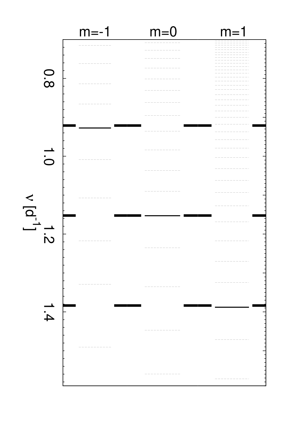
As one can see from Fig. 2, three frequencies HD 21071, i. e. , and , are dipole axisymmetric modes. The frequency can be a dipole axisymmetric or a retrograde mode, or a quadrupole retrograde mode. One can also see that , and are equally spaced in frequency. If we are not in the asymptotic regime of high order acoustic modes, which is obviously true in our case, a rotational origin of triplets is a most probable explanation for such type of structures. If we are dealing with a rotationally split triplet, the central peak, , should be an axisymmetric mode, the left side peak, , should be a retrograde mode and the right side peak, , a prograde mode. However, this is in contradiction with the identification of as an axisymmetric mode.
Another evidence suggesting the non-rotational origin of the triplet is its perfect symmetry. The difference between the central and left side peaks, , is equal within the errors to the difference between the right side and the central peaks, . Linear pulsational theory predicts an asymmetry and the left side peak should be closer to the central one than the right side peak (see also Appendix A for more details, only in the electronic edition of the journal).
Because the study of higher order effects of mode coupling is beyond the scope of this paper, we assumed that the triplet in the oscillation spectrum of HD 21071 is accidental.
4 Seismic modelling
4.1 Zero rotation-approximation

The two highest amplitude frequencies, and , are separated from each other by only 0.03909 d-1. Since from the mode identification we know they are dipole axisymmetric modes, such small separation can suggest that they are consecutive radial orders. To check this hypothesis, we constructed a preliminary grid of pulsational models in the framework of the zero-rotation approximation. We calculated models lying within the error box (see Fig. 1) for three values of metallicities, , the initial hydrogen abundances, , OP opacity tables and AGSS09 chemical mixture with a step in mass of 0.005 . No overshooting from convective core has been taken into account. It turned out that a minimal separation between consecutive radial orders of dipole modes in the frequency range appropriate for and (i.e. above 1 d-1) is d-1. This minimum theoretical separation is almost two times larger than the observed difference between and and was achieved between modes and in the model with , , and . In Fig. 3, there is shown the evolution of the frequencies of dipole modes from ZAMS to the rightmost edge of the error box. As one would expect, (marked by the two headed arrow) coincides with the avoided crossing phenomenon.
As a consequence, to properly interpret the frequencies and , one has to include effects of rotation. In the rotating star the eigenvalue is replaced by which for axisymmetric modes is increasing function of . Increasing imitates the effect of the higher degree, , and, as a consequence, the oscillation spectrum is more dense for a given frequency range.
4.2 Including rotation
In this section, we construct seismic models fitting the two (, ) and three (, , ) observed frequencies of HD 21071. The effects of rotation were included via the traditional approximation in which the effects of the Coriolis force are taken into account whereas centrifugal distortion is neglected. Rigid rotation is assumed.
The method of mode identification developed by Daszyńska-Daszkiewicz et al. (2015) allows, besides determination of and , to constrain the rotational velocity. Szewczuk & Daszyńska-Daszkiewicz (2015b) showed that the rotation rate of HD 21071 is in the range km s-1. We confine our searching of seismic models to this range of the rotational velocity. Due to a high computational cost, it was done in the two steps.
Firstly, we constructed a preliminary grid of models for , with the OP opacity data, AGSS09 chemical mixture and without overshooting from the convective core (). Models were calculated inside the error box (see Fig. 1) for different masses, metallicities and rotation velocities with a step , and km s-1. Then, to find the approximate parameters of models which fit the two observed frequencies, the theoretical frequencies were interpolated by means of multi-dimensional linear interpolation.
In the second step, around the approximate model parameters for which theoretical frequencies fit the observed ones, we computed a denser grid of models with steps and . A step in effective temperature in both grids was dynamically determined by the evolutionary code and equal approximately to .
We will call the grid of models with the input (, OP, AGSS09, ) as G1.
| G1 | G2 | G3 | G4 | |
| OP | OP | OP | OPAL | |
| 150 | ||||
| 160 | - | |||
| 170 | - | |||
| 180 | - | |||
| 190 | - | - | - | |
| 200 | - | - | - | - |
| 210 | - | - | - | |
| 220 | - | - | ||
| 230 | - | - | - | |
| 240 | - | - | - | - |
| 250 | - | - | - |


In Fig. 4, we put seismic models fitting and in the HR diagram for the seven values of . The colours are assigned to the values of metallicity, . In this figure all modes, stable and unstable, were plotted. The use of the instability condition significantly reduces the number of seismic models. Our seismic modelling showed that for km s-1 there are very few models with unstable modes which reproduce and . Moreover, these models have rather high metallicity. For example, in the case of km s-1 unstable modes reproducing and were found in models with . On the other hand, in the case of the lowest considered rotational velocity, ie., km s-1 unstable modes reproducing and were found in models with metallicity as low as .
All our seismic models of HD21071 can be divided into two families. The first one (hereafter F1), associated with the radial orders from to , has on average higher metallicity and is more luminous. The second one (hereafter F2), associated with the radial orders from to , has on average lower metallicity and is less luminous. In both cases the models which fit and become more luminous with increasing rotation velocity. For the lowest rates of rotation, i. e., and 160 km s-1, we found only models with the F1 solution within 3 error box. The seismic models from the F2 solution appear close to the lowest edge of the 3 error box () from km s-1. With increasing , we obtained more and more models from F2 and less from F1 in the space of parameters we considered. For the highest rotational velocity, km s-1, we found only seismic models from F2. In both cases, there is a clear trend: the lower metallicity the higher luminosity.
The seismic models of HD 21071 lie along sloped lines in the HR diagram. For one pair of the radial orders we usually have a few nearly parallel sequences of such models differing in metallicity. A similar structure occurs in the diagram . This is because the frequencies of the g modes in the range of parameters and frequency we consider, in general, decrease with decreasing effective temperature and increasing mass. The dependence on is varied, for the higher radial orders, , the pulsational frequency is an increasing function of , whereas for there is an oscillatory character of . In Fig. 5, for clarity, we show the diagram for only one pair of the radial orders, g14 and g15, and one value of the rotational velocity.
Gaps which sometimes appear along the lines of seismic models result from the adopted steps in and , which, although small, can cause the omission of some models.
It is worth to notice that in the case of F1 we have always consecutive radial orders whereas in the F2 solution we have every second radial order. This is because with increasing the eigenvalue of the , mode increases and as a result of denser oscillation spectrum of the high radial order modes is shifted towards higher frequencies. This explains why we have more models from F1 than F2 for lower rotation rates and vice versa. On the other hand coexistence solutions from F1 and F2 for fixed rotational velocity (e. g., km s-1) is associated with considerably different parameters of the models from both families of solutions (mainly metallicity and mass) as described in previous paragraph.
An interesting fact is that most unstable modes comes from the F1 seismic models. The only exception is for km s-1 where some modes from the F2 solution are unstable. With increasing there are less and less seismic models with unstable modes fitting the two frequencies and . On the one hand this is due to lower metallicity of the F2 models which dominate for the higher rotational velocities, on the other, for higher the instability domain is shifted towards higher frequencies than the observed ones.
In the next step we selected models which fit the third observational frequency, , which also corresponds to a dipole axisymmetric mode. Models fitting , and are shown in Fig. 6. We can see a further reduction in the number of models. Moreover, we did not find a solution for each value of . The radial orders of modes which fit , and from the G1 grid are given in the second column of Table 2. Unstable solutions exist only for km s-1.
4.3 Effects of hydrogen abundance, core overshooting and opacities
There are many input parameters, both, from a model and microphysics, that may affect pulsational frequencies. Here, we examine the influence of the initial hydrogen abundance, , overshooting from the convective core (in terms of the parameter ) and the opacities. The effect of the core overshooting was included according to the formulation of Dziembowski & Pamyatnykh (2008) which takes into account, both, the distance of the overshooting and partial mixing in the overshoot layer.
To this end we constructed three additional grids of models in the same way as explained in Section 4.2. In the second grid, G2, we used (comparing to in G1), in the third grid, G3, we added the core overshooting, , and in the fourth one, G4, we used OPAL (Iglesias & Rogers, 1996) opacity tables (instead of OP used in G1).
We found that independently of the adopted grid, all trends noted in G1 are also present in G2, G3 and G4. Firstly, there are always the two families of solutions. The first one, F1, with the radial orders of about and the second one, F2, with the radial orders of about .

With an increased abundance of hydrogen (the G2 grid), we found less seismic models compared to G1, in particular for the F2 solution.
Seismic models with and without overshooting from the convective core (G3 G1) lie approximately in the same places of the HR diagram but the G3 models are confined to slightly narrower bands. A similar picture emerges when we considered seismic models only with unstable modes.
Changing the opacity tables (G4 . G1) has very little effect on the position of seismic models in the HR diagram. The G4 models are only slightly more luminous. The same is true if only unstable modes are considered. The exception is for seismic models with km s-1. In this case, unstable modes occurs only in the F2 solution. This is opposite to seismic models calculated with the OP tables. There are fewer seismic models with unstable modes obtained with the use of the OPAL opacities. This result is not surprising as it is well known that for SPB models the computations with the OP tables give more unstable modes than those with the OPAL ones (Pamyatnykh, 1999, e.g.).
Models which fit the three frequencies , and in the grids G2, G3 and G4 are presented in Fig. 7. In Table 2, we list the allowed combinations of the radial orders.
As in the case of G1, only for the lower rotation velocity, km s-1, we were able to find models which fit the three frequencies with the instability condition fulfilled. For km s-1, the number of these seismic models is significantly lower and the modes are stable (cf. Table 2).
| Grid | opacity | ID | () | |||||||
| (km s-1) | ||||||||||
| G1 | OP | 0.70 | 0.0 | 150 | grp a | – | ||||
| G1 | OP | 0.70 | 0.0 | 150 | rep a | 0.01575 | 4.0357 | 4.15528 | 2.4554 | 0.139 |
| G1 | OP | 0.70 | 0.0 | 160 | grp b | – | ||||
| G1 | OP | 0.70 | 0.0 | 160 | rep b | 0.02340 | 4.3793 | 4.15814 | 2.4831 | 0.331 |
| G1 | OP | 0.70 | 0.0 | 170 | grp c | – | ||||
| G1 | OP | 0.70 | 0.0 | 170 | rep c | 0.01630 | 4.2221 | 4.15948 | 2.5435 | 0.312 |
| G1 | OP | 0.70 | 0.0 | 180 | grp d | – | ||||
| G1 | OP | 0.70 | 0.0 | 180 | rep d | 0.02210 | 4.3521 | 4.15492 | 2.5042 | 0.624 |
| G2 | OP | 0.75 | 0.0 | 160 | grp e | – | ||||
| G2 | OP | 0.75 | 0.0 | 160 | rep e | 0.01855 | 4.6566 | 4.17028 | 2.5304 | 0.230 |
| G2 | OP | 0.75 | 0.0 | 170 | grp f | – | ||||
| G2 | OP | 0.75 | 0.0 | 170 | rep f | 0.01375 | 4.4643 | 4.16493 | 2.5657 | 0.720 |
| G2 | OP | 0.75 | 0.0 | 180 | grp g | – | ||||
| G2 | OP | 0.75 | 0.0 | 180 | rep g | 0.01835 | 4.6040 | 4.16237 | 2.5347 | 0.003 |
| G3 | OP | 0.70 | 0.2 | 150 | grp h | – | ||||
| G3 | OP | 0.70 | 0.2 | 150 | rep h | 0.01640 | 3.9139 | 4.14568 | 2.4114 | 0.740 |
| G3 | OP | 0.70 | 0.2 | 160 | grp i | – | ||||
| G3 | OP | 0.70 | 0.2 | 160 | rep i | 0.01340 | 4.0365 | 4.16247 | 2.5255 | 0.497 |
| G3 | OP | 0.70 | 0.2 | 160 | grp j | – | ||||
| G3 | OP | 0.70 | 0.2 | 160 | rep j | 0.01740 | 4.0997 | 4.15804 | 2.4604 | 0.214 |
| G3 | OP | 0.70 | 0.2 | 160 | grp k | – | ||||
| G3 | OP | 0.70 | 0.2 | 160 | rep k | 0.02115 | 4.3860 | 4.16833 | 2.5072 | 0.326 |
| G4 | OPAL | 0.70 | 0.2 | 150 | grp l | – | ||||
| G4 | OPAL | 0.70 | 0.2 | 150 | rep l | 0.02075 | 4.0651 | 4.15081 | 2.3900 | 0.413 |
| G4 | OPAL | 0.70 | 0.2 | 180 | grp m | – | ||||
| G4 | OPAL | 0.70 | 0.2 | 180 | rep m | 0.01745 | 4.4846 | 4.18217 | 2.6091 | 0.433 |

To summarize our results of seismic modelling of the star HD 21071, in Table 3 we give the ranges of the stellar parameters of models with unstable modes which fit the three frequencies, , and , for the four grids. The parameters are provided for each separate group of models with similar properties, shown in Figs. 6 and 7 by ovals. The groups are marked as ’grp’ in Table 3. In addition, we give also the parameters of representative models for each group (marked as ’rep’ in Table 3). In the last column we give, for the representative seismic models, the goodness of the fit defined as
| (1) |
where and are observed and theoretical frequency, respectively, and are the observational errors of the frequencies.
It should be mentioned that masses of seismic models from Table 3 are in the range whereas masses of evolutionary models which fall into the 3 error box are in a slightly wider range . The range of masses of evolutionary models given above is wider than the one given in Section 2 because here we take into account models with all considered metallicities () and from all grids.
In Fig. 8, we compare the oscillation spectrum of HD 21071 with the theoretical spectra corresponding to the representative seismic models from Table 3. In the bottom panel of Fig. 8, we show a zoom-in on the frequencies around the observed values. As one can see, the model G2g reproduces also the frequency within the observational errors if it is the mode , g22, a possibility consistent with our mode identifications. Similarly, the quadrupole retrograde mode , g38 in the model G3i fits the frequency . This mode is also allowed by our mode identifications.
We can also see that the frequency of the mode , g22 is close to in the models G1d and G4m. In a similar distance is also the mode, , g31, in the model G3k. Given the numerical accuracy of theoretical frequencies, which is about d-1, we have to accept also these solutions. The important result is that these identifications are valid for the all seismic models constructed in this paper.
5 Conclusions
This paper focused on the challenges and prospects for seismic modelling of slowly pulsating B-type stars with the effects of rotation taken into account. We used as an example the star HD 21071 which pulsates in four frequencies of which the three have a unique mode identification. Firstly, we showed that non-rotating models cannot account for the two highest amplitude frequencies, and d-1, and including the effects of rotation on high-order g modes is indispensable. Then, having unambiguous determination of the two angular numbers for the three observed frequencies of HD 21071 (, and d-1), and constraints on the range of the rotational velocity, km s-1, we constructed rotating seismic models which reproduce these three frequencies. We examined the effects of the initial abundance of hydrogen, an amount of the core overshooting and the opacity data, considering four grids of parameters. Due to the high density of the theoretical oscillation spectra, a large number of solutions have been obtained. Despite of that, only two combinations of the radial orders, , were allowed: one set is around and the second one around . Moreover, the instability condition reduced the number of seismic models significantly. Therefore, accurate calculations of the opacity data are of the utmost importance.
Among seismic models fitting the three frequencies, we found some that reproduce also the forth frequency, d-1. In all grids of models only the dipole axisymmetric modes g22 or quadrupole modes , g38, g31 have frequencies close to (given the observational errors and numerical accuracy). Both modes are in agreement with the mode identification. Fitting the forth frequency further reduced the number of seismic models. However, to derive more stringent constraints on opacities, core overshooting etc. more well identified frequencies are necessary. Because we tried to constrain seven parameters (), we need at least seven well identified pulsational frequencies.
There are many SPB stars with far more rich oscillation spectra obtained from the space missions, like MOST, CoRoT and Kepler, but the problem is their mode identification. Even if there are some patterns in the oscillation spectra, they can be accidental, i.e., composed of modes with different pairs (), and cannot be interpreted in term of the asymptotic theory (Szewczuk, Daszyńska-Daszkiewicz & Dziembowski, Szewczuk et al.2014). Therefore, except for the excellent example of KIC 10526294 with 19 consecutive rotationally split dipole modes (Pápics et al., 2014), there is no other reliable seismic modelling of an SPB star.
The aim of this paper was to show that seismic modelling of SPB stars is feasible even if no asymptotic pattern is observed in the oscillation spectra and a limited number of modes is detected, provided the angular numbers are determined unambiguously and the effects of rotation are properly included. Therefore, a hope is pinned on the two colour data from the BRITE mission which, besides more frequencies and better accuracy, can be used to identify the pulsational modes.
Acknowledgments
We gratefully thank Mike Jerzykiewicz for his carefully reading the manuscript. WS was financially supported by the Polish NCN grant DEC-2012/05/N/ST9/03905 and JDD by the Polish NCN grants 2011/01/M/ST9/05914, 2011/01/B/ST9/05448. Calculations have been carried out using resources provided by Wrocław Centre for Networking and Supercomputing (http://wcss.pl), grant No. 265
References
- Abt & Hunter (1962) Abt H.A., Hunter Jr.J.H., 1962, ApJ, 136, 381
- Abt et al. (2002) Abt H.A., Levato H., Grosso M., 2002, ApJ, 573, 359
- Aerts et al (1992) Aerts C., de Pauw M., Waelkens C., 1992, A&A, 266, 294
- (Andrews et al.2003) Andrews J.E., Dukes R.J., Mills L.R., 2003AAS…203.8314
- Asplund et al. (2009) Asplund M., Grevesse N., Sauval A.J., Scott P., 2009, ARA&A, 47, 481
- Ballot et al. (2012) Ballot J., Lignieŕes F., Prat V., Reese D.R., Rieutord M., 2012, in Shibahashi H., Takata M., Lynas-Gray A.E., eds, ASP Conf. Ser. 462, Progress in Solar/Stellar Physics with Helio- and Asteroseismology. Astron. Soc. Pac., San Francisco, p. 389
- Balona (1986a) Balona L.A.,1986a, MNRAS, 219, 111
- Balona (1986b) Balona L.A.,1986b, MNRAS, 220, 647
- Balona & Stobie (1979) Balona L.A., Stobie R.S., 1979, MNRAS, 189, 649
- Briquet et al (2007) Briquet M., Hubrig S., De Cat P., Aerts C., North P., Schöller M., 2007, A&A, 466, 269
- Campos & Smith (1980a) Campos A.J., Smith M.A., 1980a, ApJ, 238, 250
- Campos & Smith (1980b) Campos A.J., Smith M.A., 1980b, ApJ, 238, 667
- Cugier & Daszyńska (2001) Cugier H., Daszyńska J., 2001, A&A, 377, 113
- Cugier et al. (1994) Cugier H., Dziembowski W.A., Pamyatnykh A.A., 1994, A&A, 291, 143
- Daszyńska-Daszkiewicz et al. (2015) Daszyńska-Daszkiewicz J., Dziembowski W.A., Jerzykiewicz M., Handler G., 2015, MNRAS, 446, 1438
- (Daszyńska-Daszkiewicz et al.2007) Daszyńska-Daszkiewicz J., Dziembowski W.A., Pamyatnykh A.A., 2007, Acta Astron., 57, 11
- De Cat (2002) De Cat P., 2002, in Aerts C., Bedding T.R., Christensen-Dalsgaard, J., eds, ASP Conf. Ser. 259, IAU Colloq. 185: Radial and Nonradial Pulsationsn as Probes of Stellar Physics. Astron. Soc. Pac., San Francisco, p. 196
- De Cat et al. (2007) De Cat P. et al., 2007, A&A, 463, 243
- Degroote et al. (2010) Degroote P. et al., 2010, Nature, 464, 259
- Dukes et al. (2003) Dukes Jr.R.J., Kubinec W.R., Kubinec A., Adelman S.J., 2003, AJ, 126, 370
- (Dziembowski et al.1993) Dziembowski W.A., Moskalik P., Pamyatnykh A.A., 1993, MNRAS, 265, 588
- Dziembowski & Pamyatnykh (2008) Dziembowski W.A., Pamyatnykh A.A., 2008, MNRAS, 385, 2061
- Freire Ferrero et al (2012) Freire Ferrero R., Morales Durán C., Halbwachs J.-L., Cabo Cubeiro A.M., 2012, AJ, 143, 28
- Gautschy & Saio (1993) Gautschy A., Saio H., 1993, MNRAS, 262, 213
- Gies & Kullavanijaya (1988) Gies D.R., Kullavanijaya A., 1988, ApJ, 326, 813
- Iglesias & Rogers (1996) Iglesias C.A., Rogers F.J., 1996, ApJ, 464, 943
- Iglesias et al. (1992) Iglesias C.A., Rogers F.J., Wilson B.G., 1992, ApJ, 397, 717
- Kennelly & Walker (1996) Kennelly E.J., Walker G.A.H., 1996, PASP, 108, 327
- Lee (2001) Lee U., 2001, ApJ, 557, 311
- Lee & Saio (1989) Lee U., Saio H., 1989, MNRAS, 237, 875
- Lee & Saio (1997) Lee U., Saio H., 1997, ApJ, 491, 839
- Lefever et al. (2010) Lefever K., Puls J., Morel T., Aerts C., Decin L., Briquet M., 2010, A&A, 515, 74
- Lesh (1968) Lesh J.R., 1968, ApJS, 17, 371
- Mathias et al. (2001) Mathias P., Aerts C., Briquet M., De Cat P., Cuypers J., Van Winckel H., Le Contel J.M., 2001, A&A, 379, 905
- (McDonald2012) McDonald I., Zijlstra A.A., Boyer M.L., 2012, MNRAS, 427, 343
- Mooley et al. (2013) Mooley K., Hillenbrand L., Rebull L., Padgett D., Knapp G., 2013, ApJ, 771, 110
- (Morgan et al1971) Morgan W.W., Hiltner W.A., Garrison R.F., 1971, AJ, 76, 242
- Niemczura (2003) Niemczura E., 2003, A&A, 404, 689
- Pamyatnykh (1999) Pamyatnykh A. A., 1999, Acta Astron., 49, 119
- Pamyatnykh et al. (1998) Pamyatnykh, A.A., Dziembowski W.A., Handler G., Pikall H., 1998, A&A, 333, 141
- Pápics et al. (2012) Pápics P. I. et al.,2012, A&A, 542, 55
- Pápics et al. (2014) Pápics P.I., Moravveji E., Aerts C., Tkachenko A., Triana S.A., Bloemen S., Southworth J., 2014, A&A, 570, 8
- Pápics et al. (2015) Pápics P. I., Tkachenko A., Aerts C., Van Reeth T., De Smedt K., Hillen M., Østensen R., Moravveji E., 2015, ApJL, 803, 25
- Reed (2005) Reed B.C., 2005, AJ, 130, 1652
- Saffe & Levato (2014) Saffe C., Levato H., 2014, A&A, 562, 128
- Seaton (2005) Seaton M.J., 2005, MNRAS, 362, 1
- Silaj & Landstreet (2014) Silaj J., Landstreet J.D., 2014, A&A, 566, 132
- Stamford & Watson (1981) Stamford P.A., Watson R.D., 1981, Ap&SS, 77, 131
- Szewczuk & Daszyńska-Daszkiewicz (2015a) Szewczuk W., Daszyńska-Daszkiewicz J., 2015, in Meynet G., Georgy C., Groh J. H., Stee Ph., eds, Proc. IAU Symp. 307, New Windows on Massive Stars: Asteroseismology, Interferometry, and Spectropolarimetry. Cambridge Univ. Press, Cambridge, p. 232
- Szewczuk & Daszyńska-Daszkiewicz (2015b) Szewczuk W., Daszyńska-Daszkiewicz J. 2015, MNRAS, 450, 1585
- (Szewczuk et al.2014) Szewczuk W., Daszyńska-Daszkiewicz J., Dziembowski W., 2014 in Guzik J.A., Chaplin W.J., Handler G., Pigulski A., eds, Proc. IAU Symp. 301, Precision Asteroseismology. Cambridge Univ. Press, Cambridge, p. 109
- Townsend (2003a) Townsend R.H.D., 2003a, MNRAS, 340, 1020
- Townsend (2003b) Townsend R.H.D., 2003b, MNRAS, 343, 125
- Townsend (2005) Townsend R.H.D., 2005, MNRAS, 360, 465
- Waelkens (1991) Waelkens C., 1991, A&A, 246, 453
- Waelkens et al. (1998) Waelkens C., Aerts C., Kestens E., Grenon M., Eyer L., 1998, A&A, 330, 215
- (Walczak et al.2012) Walczak P., Szewczuk W., Daszyńska-Daszkiewicz J., 2012, Astrono. Nachr., 333, 1065
- (Walczak et al.2013) Walczak P., Szewczuk W., Daszyńska-Daszkiewicz J., 2013, in Suárez J.C., Garrido R., Balona L.A., Christensen-Dalsgaard J., eds, Astrophysics and Space Science Proceedings Vol. 31: Stellar Pulsations: Impact of New Instrumentation and New Insights. Springer-Verlag Berlin Heidelberg, p. 191
- Watson (1988) Watson R.D., 1988, Ap&SS, 140, 255
- Telting & Schrijvers (1997) Telting J.H., Schrijvers C., 1997, A&A, 317, 723
- Zorec & Royer (2012) Zorec J., Royer F., 2012, A&A, 537, 120
Appendix A Asymmetry of the rotationally split modes in the framework of the traditional approximation
Linear theory of pulsation predicts asymmetry between rotationally split components of the given mode, ie., retrograde modes should be closer to the axisymmetric ones than prograde modes. In Table 4 we list frequencies of dipole modes and the differences between their components for the model at the centre of the error box (, , , , , ). The rotation splitting was computed with the traditional approximation and the rotational velocities were chosen to approximately reproduce the value of the observed splitting in HD 21071. As one can see, in all cases retrograde modes are closer to axisymmetric modes than prograde ones and asymmetry is of the order of 0.01 d-1. This property is also clearly seen in Fig. 9, where the observed triplet is compared with the theoretical spectrum calculated for the model at the centre of error box of HD 21071. The observed frequencies were shifted in order to align the central peak, , with the mode.
| 60 | 13 | 0.86855 | 1.08271 | 1.30635 | 0.21416 | 0.22364 |
|---|---|---|---|---|---|---|
| 12 | 0.93075 | 1.14612 | 1.37041 | 0.21537 | 0.22429 | |
| 11 | 1.01204 | 1.22871 | 1.45373 | 0.21667 | 0.22502 | |
| 10 | 1.11148 | 1.32946 | 1.55497 | 0.21798 | 0.22551 | |
| 62 | 13 | 0.86667 | 1.08742 | 1.31828 | 0.22075 | 0.23086 |
| 12 | 0.92855 | 1.15066 | 1.38221 | 0.22211 | 0.23155 | |
| 11 | 1.00942 | 1.23300 | 1.46530 | 0.22358 | 0.23230 | |
| 10 | 1.10854 | 1.33333 | 1.56619 | 0.22479 | 0.23286 | |
| 65 | 13 | 0.86408 | 1.09459 | 1.33623 | 0.23051 | 0.24164 |
| 12 | 0.92547 | 1.15755 | 1.39986 | 0.23208 | 0.24231 | |
| 11 | 1.00584 | 1.23941 | 1.48263 | 0.23357 | 0.24322 | |
| 10 | 1.10431 | 1.33940 | 1.58344 | 0.23509 | 0.24404 |