Determining Optimal Test Functions for Bounding the Average Rank in Families of -FunctionsThanks: This research was supported by NSF grants DMS1265673 and Williams College. We thank Eyvi Palsson, Mihai Stoiciu, and the referee for helpful comments and discussions.
Abstract.
Given an -function, one of the most important questions concerns its vanishing at the central point; for example, the Birch and Swinnerton-Dyer conjecture states that the order of vanishing there of an elliptic curve -function equals the rank of the Mordell-Weil group. The Katz and Sarnak Density Conjecture states that this and other behavior is well-modeled by random matrix ensembles. This correspondence is known for many families when the test functions are suitably restricted. For appropriate choices, we obtain bounds on the average order of vanishing at the central point in families. In this note we report on progress in determining the optimal test functions for the various classical compact groups for different support restrictions, and discuss how this relates to improved rank bounds.
Key words and phrases:
Random matrix theory, -functions, low-lying zeros, optimal test functions2010 Mathematics Subject Classification
Primary: 11Mxx; Secondary: 45Bxx1. Introduction
1.1. Background
While the importance of random matrices in mathematics and related disciplines had been noticed at least as early as Wishart’s work [Wis] in the late 1920s, for us in number theory the story begins with the connections observed by Montgomery and Dyson [Mon] in the 1970s. Montgomery was studying the pair-correlation of zeros of the Riemann zeta function, and the behavior was identical to that of certain random matrix ensembles which had been extensively studied due to their applicability in nuclear physics. Briefly, characteristic polynomials (and their eigenvalues) of the classical compact groups have been observed to model well -functions (and their critical zeros). While we will concentrate on low-lying zeros, i.e., zeros near the central point, in families of -functions, there is an extensive literature on other statistics, including -level correlations [Hej, Mon, RS], spacings [Od1, Od2], and moments [CFKRS]. See [FM, Ha] for a brief history of the subject and [Con, For, KaSa1, KaSa2, KeSn1, KeSn2, KeSn3, Meh, MT-B, T]) for some articles and textbooks on the connections.
In many of the earlier works on the correspondences between the two subjects, the statistics studied were insensitive to the behavior of finitely many zeros. This led to the introduction of a new statistic, the -level density, as often the zeros near the central point are related to important arithmetic quantities, with the Birch and Swinnerton-Dyer conjecture (stating that the order of vanishing of the -function at the central point equals the rank of the Mordell-Weil group of rational solutions) the most famous example. In this paper we concentrate on the -level density, which we define in detail in §1.2. We report on recent results from the first author’s honors thesis at Williams College, supervised by the second author, where building on methods introduced in [ILS] optimal test functions are constructed for various statistics for different support ranges. The main application of these theorems are improved estimates on the average vanishing at the central point for families of -functions. In addition to being of general interest, such results have important applications (for example, in [IS] good estimates here are connected to the Landau-Siegel zero question).
In the arguments below we concentrate on the limiting behavior. An important topic for future research is to include lower order terms and determine the optimal test functions for various regimes where the limiting behavior has not yet been reached. These regimes are quite important as they are the ones that can be investigated numerically, and often the data gathered is at odds with the limiting predictions as the rate of convergence is abysmally slow. The prime example is that of whether or not their is excess rank in families of elliptic curves (see [BMSW] for a nice summary of data and conjectures); while earlier investigations indicated that such bias might persist, later studies [W] went far enough to see the average rank drop, and new random matrix models have been introduced that have the correct limiting behavior and successfully model the observed behavior for small conductors [DHKMS1, DHKMS2]. There are now many results on lower order terms in families, such as [HKS, MMRW, Mil2, Yo1], and the hope is that the methods of this paper can be extended to include these to refine estimates for finite conductors.
On a personal note, the second author investigated questions on rates of convergence with Ram Murty in [MM] (explicitly, proving effective bounds on families of elliptic curves modulo (for prime tending to infinity) obeying the Sato-Tate Law). It is a pleasure to dedicate this work to him on the occasion of his 60th birthday, and we hope to report on extending our result to lower order terms before his next big celebration!
1.2. -Level Density
As alluded to above, the behavior of zeros far from the central point exhibit a remarkable universality across -functions. Unfortunately it is significantly harder to study one -function’s zeros near the central point. The reason is that there are only a few normalized zeros near the central point, and there is thus no possibility of averaging if we restrict ourselves to just one object (in the extreme case of whether or not the -function vanishes, we just have a ‘yes-no’ question). To make progress, we instead study a family of -functions. The Katz-Sarnak philosophy [KaSa1, KaSa2] states that the behavior of a family of -functions should be well-modeled by a corresponding classical compact groups, with the conductor in the family tending to infinity playing the same roll as the growing matrix size; for alternative approaches to modeling the behavior of zeros, see [CFZ1, CFZ2, GHK].
We briefly describe the main statistic studied, the -level density (though we will report on progress on the 1-level only here, see [F] for additional results). For ease of exposition we assume the Generalized Riemann Hypothesis, so given an all the zeros are of the form with real. Our statistic makes sense more generally, but we lose the interpretation of ordered zeros and connections with nuclear physics; the main use of GRH is to extend the support calculation for many of the number theory computations. We assume the reader is familiar with -level densities; for more detail on these statistics see the seminal work by Iwaniec, Luo and Sarnak [ILS], who introduced them, or [AAILMZ] for an expanded discussion (which formed the basis of the quick summary below).
Let where each is an even Schwartz function such that the Fourier transforms
| (1.1) |
are compactly supported. The -level density for with test function is
| (1.2) |
where is a scaling parameter which is frequently related to the conductor. Given a family of -functions with conductors tending to infinity, the -level density with test function and non-negative weight function is defined by
| (1.3) |
Frequently one chooses to be either all forms with conductor equal to , or conductor at most .
Unlike the -level correlations of a family, which have a universal limit as the height of the zero tends to infinity, Katz and Sarnak [KaSa1, KaSa2] proved that the -level density is different for each classical compact group. They were able to obtain closed form determinant expansions; while these expressions can be hard to use for (see [HM] for a discussion on the benefits of an alternative), they are very easy to use for the 1-level.
Let and for . If is the family of unitary, symplectic or orthogonal families (split or not split by sign), the -level density for the eigenvalues converges as to
| (1.4) |
where
| (1.5) |
While these densities are all different, for the 1-level density with test functions whose Fourier transforms are supported in , the three orthogonal flavors cannot be distinguished from each other in this regime, though they can be distinguished from the unitary and symplectic.
In many of the calculations it is convenient to shift to the Fourier transform side. Letting
| (1.6) |
and denote the standard Dirac Delta functional, for the -level densities we have
| (1.7) |
Note that the first three densities agree for and split (i.e., become distinguishable) for ; alternatively, one could use the 2-level density which suffices to distinguish all candidates for arbitrarily small support (see [Mil2]).
As stated earlier, the Katz-Sarnak Density Conjecture is that the behavior of zeros near the central point in a family of -functions (as the conductors tend to infinity) agrees with the behavior of eigenvalues near 1 of a classical compact group (as the matrix size tends to infinity). There is now an extensive body of work supporting this for numerous families and various levels of support, including Dirichlet characters, elliptic curves, cuspidal newforms, symmetric powers of -functions, and certain families of and -functions; see for example [DM1, DM2, ER-GR, FiM, FI, Gao, Gü, HM, HR, ILS, KaSa2, LM, Mil1, MilPe, OS1, OS2, RR, Ro, Rub, Ya, Yo2]. This correspondence between zeros and eigenvalues allows us, at least conjecturally, to assign a definite symmetry type to each family of -functions (see [DM2, ShTe] for more on identifying the symmetry type of a family).
1.3. Main Result
One of the most important applications of the -level density is to estimate the average order of vanishing of -functions at the central point in a family; this is the analytic rank, and is denoted . While in some families it is natural to use slowly varying weights (such as the Petersson weights for families of holomorphic cusp forms), with additional work these weights can often be removed (see [ILS]).
If we assume GRH for our family of -functions, then all critical zeros have real part 1/2. Further, if our test function is non-negative, then in the -level density we obtain an upper bound for the average rank by removing the contribution from all zeros not at the central point:
| (1.8) |
In practice, we can only establish the -level density for test functions with restricted support. On the number theory side, the goal is to verify the correspondence for as large of support as possible, as we can then use (1.8) to bound the rank:
| (1.9) |
Note that instead of trying to increase the support for the 1-level density we could shift to studying higher level densities. While this gives us better bounds for high vanishing at the central point, the probability of vanishing to order or higher decays like , unfortunately grows with and the result is worse than the bounds from the 1-level density for small (which are the ones we care about most); see [HM].
Using the Paley-Wiener theorem to note the admissible test functions are the modulus squared of an entire function of exponential type 1 (or its Fourier transform as a convolution), Plancherel’s theorem to convert to an equivalent minimization problem, and some Fredholm theory, in Appendix A of [ILS] the optimal test functions are computed for the 1-level density for the classical compact groups under the assumption that the support of the Fourier transform is contained in . Our main result is to generalize these computations to larger support and higher .
Theorem 1.1.
Let be an even Schwartz test function such that , with . Then for the test function which minimizes the right hand side of (1.8) is given by . Here represents convolution, , and is given by
| (1.10) |
and
| (1.11) |
for , and
| (1.12) |
for or . Here, the and are easily explicitly computed, and are given later in (5.9), (5.10), (5.11), (5.12), and (5.13).
For the rest of the paper, we let . Unless otherwise stated, , corresponding to the range for . This notation is slightly at odds with other works in the literature, where the support of is contained in and for us it is ; we have elected to proceed this way as the natural object is , and the support of is double that of .
Moreover, the optimal function , along with its coefficients and its scaling factor , all depend on . As this will be clear from equations (5.9) to (5.13), to simplify the notation we often omit the subscript or , as these are fixed in the analysis.
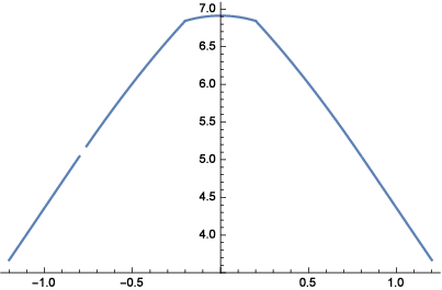
To help illustrate the main theorem, we include plots of the optimal for the groups SO(even), SO(odd), and Sp below in Figure 1, and the plots for the corresponding optimal in Figure 2; we do not include the optimal plots for the mixed orthogonal case, as the resulting is constant.



As an immediate corollary we obtain the following bounds on the average rank. We isolate these upper bounds below. The record for largest support for the 1-level density are families of cuspidal newforms [ILS] and Dirichlet -functions [FiM] (though see also [AM] for Maass forms), where we can take . It is possible to obtain better bounds on vanishing by using the 2 or higher level densities, though as remarked above in practice the reduced support means these results are not better than the 1-level for extra vanishing at the central point but do improve as we ask for more and more vanishing (see [HM]).
Corollary 1.2.
Let be a family of -functions such that, in the limit as the conductors tend to infinity, the 1-level density is known to agree with the scaling limit of unitary, symplectic or orthogonal matrices. Then for every in the limit the average rank is bounded above by
| (1.13) |
|
Remark 1.3.
We only list and not the optimal test functions or their Fourier transforms above, as we do not need either function for the computation of the infimum. [ILS] show that given the associated to the optimal function, the infimum is given by
| (1.14) |
where the integral above exists and is nonzero by (1.17) and (2.4), both established later.
A natural choice for a test function is the Fourier pair
| (1.15) |
this is the function used for the initial computation of average rank bounds in [ILS] and are optimal for . For the groups , and for the functions we find provide a significant improvement for the upper bounds on average rank over the pair (1.15). We illustrate the improvement in Figure 3, which is much easier to process than (1.13).


1.4. Sketch of Proof
The first step in our proof is to note that it follows from the Paley-Wiener theorem and Ahiezer’s theorem that the admissible functions , with satisfy
| (1.16) |
where
| (1.17) |
see Appendix A of [ILS]. We will sometimes refer to an “optimal ”. By this, we mean the that satisfies (1.16) and (1.17) for the optimal at a fixed level of support.
The broad strategy of the proof of Theorem 1.1 is to use an operator equation from [ILS] to show (non-constructively) that for all , there exists a unique optimal test function with that minimizes the functional
| (1.18) |
We then find a collection of necessary conditions that leave us with precisely one choice for .
More explicitly, our argument proceeds as follows.
- (1)
We show that certain optimality criterion on presented in [ILS] holds for all (here .
- (2)
We show that is smooth almost everywhere, where and .
- (3)
Our kernels give us a series of location-specific integral equations. Using the previous smoothness result, we convert those to a system of location-specific delay differential equations.
- (4)
We solve this system to find an -parameter family in which our solution lives. To find this solution, we incorporate symmetries of – namely that it is even.
- (5)
Incorporating more necessary conditions on , we reduce the family to a single candidate function – by our existence result this is our , from which we obtain our optimal test function .
From the list above, we will accomplish goal 1 in §2, goal 2 in §3, goal 3 in §4.1, goal 4 in §4.2, and goal 5 in §5. The proof of the optimal functions for is significantly easier than the proofs for the other functions. We include a brief proof of this fact at the end of §3. Finally, we conclude with some remarks about how these results are used in number theory, and discuss ongoing and future research.
2. Extension of the Conditions of [ILS]
Our first step is to state and extend an optimality criterion on , analogous to that in Appendix A of [ILS] (we will state it in (2.4)). Following their arguments, we seek to minimize the functional
| (2.1) |
where is the identity operator,
| (2.2) |
and
| (2.3) |
where is the indicator function for the interval .
Lemma 2.1.
The operator is compact for all , and all choices of .
Proof.
As the functions in (2.3) are all clearly in , they are trace class and therefore compact. ∎
It follows that the operator satisfies the Fredholm alternative for all and all . Applying the arguments from [ILS] shows that for all the operator is still positive definite. Thus there is some such that
| (2.4) |
Again, following the arguments of [ILS], one can show that this indeed minimizes (2.1). This completes the first step.
We are now ready to find the optimal functions for .
Lemma 2.2.
For , and for any , the optimal test function for the minimization of (1.18) is
| (2.5) |
and the associated upper bound on average rank is
| (2.6) |
3. Smoothness Almost Everywhere
We now show that for an optimal such that , must be Lipschitz continuous. Then we show that such a function is differentiable almost everywhere, using a theorem of Rademacher.
First, we show that is bounded.
Lemma 3.1.
Proof.
We show that
| (3.1) |
is bounded. We know that . By the Cauchy-Schwarz inequality, we have
| (3.2) |
and thus is bounded.
By (2.4), we know that for the optimal we have . As is bounded the optimal must bounded. ∎
Proposition 3.2.
For any , the optimal is Lipschitz continuous.
Proof.
Using (2.4) and applying the maximum modulus inequality, we see that for ,
| (3.3) |
We now analyze (3.3). Notice that for all choices of in (2.3), the integrand is bounded by 1/2. We will examine the region of integration. Without loss of generality we may assume . Note that our integrand vanishes everywhere except from to and again from to . Thus the region of integration has measure at most , and the integrand vanishes outside of a set of measure at most .
We may now revise the inequality in (3.3):
| (3.4) |
completing the proof that is a Lipschitz continuous function. ∎
We use a theorem of Rademacher to show that our function is differentiable almost everywhere.
Theorem 3.3 (Rademacher (see Theorem 3.1.6 of [Fed])).
Let be open. If is Lipschitz continuous, then is differentiable almost everywhere in .
We immediately obtain the following.
Corollary 3.4.
For all , the optimal is differentiable almost everywhere.
Proof.
Finally, we show that each such is in fact infinitely differentiable almost everywhere.
Lemma 3.5.
The optimal is infinitely differentiable almost everywhere.
Proof.
We proceed by induction. Our base case, that is once-differentiable, is established by Corollary 3.4. For the inductive step, we assume that is -times differentiable.
Note that for any choice of , we have
| (3.5) |
where the are scalars and is either a constant or a smooth function of . In particular, for at least one of the is a smooth function of . We know that is continuous. By the fundamental theorem of calculus and the chain rule, the expression on the righthand side of (3.5) is times differentiable. This completes the proof of the inductive step, and thus is smooth almost everywhere. ∎
4. A System of Integral Equations
To establish our integral equations, we first show that the optimal is even.
Lemma 4.1.
The optimal is even.
Proof.
By the results of the previous section, finding the optimal for involves finding the optimal for . We claim, (momentarily without justification) that there are three intervals of importance in our study of this function. These are
| (4.2) |
As is even, it suffices to find on , which means finding on all of the intervals above. Examining the kernels in (2.3) and the requirement (2.4), we see that for , the optimal satisfies
| (4.3) |
and for or , we have
| (4.4) |
In equations (4.3) and (4.4), we note that for and for and for and for or .
4.1. Conversion to Location-Specific System of Delay Differential Equations
4.2. Solving The System
Lemma 4.2.
The optimal satisfies
| (4.7) |
for some .
Before proving this lemma, it is important to note the following symmetry among our intervals. We first set some notation. If is a number and is an interval,
| (4.8) |
Note that is one of the intervals defined in
| (4.9) |
We also mention that
| (4.10) |
though we will not use this fact until later.
Proof.
Note that because of the symmetry (4.10), the associated delay differential equation on interval two is different. It is
| (4.14) |
Lemma 4.3.
The delay differential equation (4.14) has a unique one-parameter family of solutions in the class . That family is
| (4.15) |
with .
Proof.
Differentiate (4.14) to obtain
| (4.16) |
where we obtain the second equality by applying (4.14) to . The third equality is simply a subsitution for . However, equation (4.16) is a standard linear differential equation that has a two-parameter family of solutions given by
| (4.17) |
We now apply (4.14) to narrow this family down to a one-parameter family. The differential equation (4.14) and trigonometric angle addition formulae yield the relation
| (4.18) |
In order for the expression above to vanish, we need the coefficients on and to both be zero. This translates into the requirement that the vector be in the nullspace of the matrix
| (4.19) |
Note the matrix in (4.19) has determinant
| (4.20) |
because . We know from [ILS] that for each the function in (4.15) is a solution to (4.14). From our determinant argument, we know all solutions to that differential equation are all scalar multiples of a single nonzero solution, completing the proof. ∎
5. Finding Coefficients
Substituting values for for , we find
| (5.1) |
|
for and
| (5.2) |
for or Sp.
Lemma 5.1.
Proof.
We use (2.4) and Lemma 3.5 to find more necessary conditions on such a . In particular, we impose the three relations:
| (5.3) | ||||
| (5.4) | ||||
| (5.5) |
The first gives continuity, the second and third ensure that is constant; however, they do not ensure it is 1. That is accomplished by using to appropriately scale down the function. This gives us the matrix equations
| (5.6) |
|
for and
| (5.7) |
|
for or . Here, is restricted to .
Expanding these matrices along the their third columns, we see that
| (5.8) |
which are both nonzero for . Solving the matrix equations, we obtain
| (5.9) |
and
| (5.10) |
for or .
We currently have for some constant . Here, is the unscaled optimal function. As some of our are nonzero and the operator is positive definite, this constant is nonzero and it can therefore be scaled to be one. We find the correct scaling factor by computing , setting that equal to in (5.1) and (5.2). From these computations, we find
| (5.11) | |||||
for , and
| (5.12) | |||||
for , and
| (5.13) | |||||
for , completing the proof. ∎
6. Conclusion and Future Work
In [F] we include similar calculations for . We conjecture that these methods will provide solutions for all . In this pursuit, there are two important steps. The first is solving the system of delay differential equations. This gives a family of solutions. The second is taking the output of that system and finding the correct system of equations that give us the coefficients to pick our optimal out of that family. Preliminary calculations suggest the second step will be more difficult than the first; however, even solving the first problem in general, or providing an algorithmic approach, is important progress as it reduces the problem to an optimization over a finite-dimensional space, as opposed to an infinite dimensional one.
While currently the best results (assuming no more than GRH) for showing agreement between number theory and random matrix theory for the 1-level density are only for , in some cases larger support is attainable through additional assumptions. One example is the slight improvement for cuspidal newforms in [ILS] under their Hypothesis S. Another are families of Dirichlet characters, where Fiorilli-Miller [FiM] improve up to under some weak assumptions about the distribution of primes in residue classes (with stronger ones arbitrarily large support is attained). Thus there are already situations where we can gainfully employ these new optimal test functions in these expanded regimes.
Additionally in [F] we hope to generalize these arguments to the -level densities, and then either there or in future work examine the slight modifications needed in the optimal function if we have lower order terms.
References
- [AAILMZ] L. Alpoge, N. Amersi, G. Iyer, O. Lazarev, S. J. Miller and L. Zhang, Maass waveforms and low-lying zeros, to appear in the Springer volume Analytic Number Theory: In Honor of Helmut Maier’s 60th Birthday.
- [AM] L. Alpoge and S. J. Miller, The low-lying zeros of level 1 Maass forms, Int. Math. Res. Not. IMRN 2010, no. 13, 2367–2393.
- [BMSW] B. Bektemirov, B. Mazur, W. Stein and M. Watkins, Average ranks of elliptic curves: Tension between data and conjecture, Bull. Amer. Math. Soc. 44 (2007), 233–254.
- [Con] J. B. Conrey, -Functions and random matrices. Pages 331–352 in Mathematics unlimited — 2001 and Beyond, Springer-Verlag, Berlin, 2001.
- [CFKRS] J. B. Conrey, D. Farmer, P. Keating, M. Rubinstein and N. Snaith, Integral moments of -functions, Proc. London Math. Soc. (3) 91 (2005), no. 1, 33–104.
- [CFZ1] J. B. Conrey, D. W. Farmer and M. R. Zirnbauer, Autocorrelation of ratios of -functions, Commun. Number Theory Phys. 2 (2008), no. 3, 593–636.
- [CFZ2] J. B. Conrey, D. W. Farmer and M. R. Zirnbauer, Howe pairs, supersymmetry, and ratios of random characteristic polynomials for the classical compact groups, preprint, http://arxiv.org/abs/math-ph/0511024.
- [DHKMS1] E. Dueñez, D. K. Huynh, J. C. Keating, S. J. Miller and N. Snaith, The lowest eigenvalue of Jacobi Random Matrix Ensembles and Painlevé VI, Journal of Physics A: Mathematical and Theoretical 43 (2010) 405204 (27pp).
- [DHKMS2] E. Dueñez, D. K. Huynh, J. C. Keating, S. J. Miller and N. Snaith, Models for zeros at the central point in families of elliptic curves (with Eduardo Dueñez, Duc Khiem Huynh, Jon Keating and Nina Snaith), J. Phys. A: Math. Theor. 45 (2012) 115207 (32pp).
- [DM1] E. Dueñez and S. J. Miller, The low lying zeros of a and a family of -functions, Compositio Mathematica 142 (2006), no. 6, 1403–1425.
- [DM2] E. Dueñez and S. J. Miller, The effect of convolving families of -functions on the underlying group symmetries,Proceedings of the London Mathematical Society, 2009; doi: 10.1112/plms/pdp018.
- [ER-GR] A. Entin, E. Roditty-Gershon and Z. Rudnick, Low-lying zeros of quadratic Dirichlet -functions, hyper-elliptic curves and Random Matrix Theory, Geometric and Functional Analysis 23 (2013), no. 4, 1230–1261.
- [FiM] D. Fiorilli and S. J. Miller, Surpassing the Ratios Conjecture in the 1-level density of Dirichlet -functions, Algebra & Number Theory Vol. 9 (2015), No. 1, 13–52.
- [FM] F. W. K. Firk and S. J. Miller, Nuclei, Primes and the Random Matrix Connection, Symmetry 1 (2009), 64–105; doi:10.3390/sym1010064.
- [F] J. Freeman, Fredholm theory and optimal test functions for detecting central point vanishing over families of -functions, Williams College honors thesis (supervised by S. J. Miller), 2015.
- [For] P. Forrester, Log-gases and random matrices, London Mathematical Society Monographs 34, Princeton University Press, Princeton, NJ 2010.
- [FI] E. Fouvry and H. Iwaniec, Low-lying zeros of dihedral -functions, Duke Math. J. 116 (2003), no. 2, 189-217.
- [Gao] P. Gao, -level density of the low-lying zeros of quadratic Dirichlet -functions, Ph. D thesis, University of Michigan, 2005.
- [GHK] S. M. Gonek, C. P. Hughes and J. P. Keating, A Hybrid Euler-Hadamard product formula for the Riemann zeta function, Duke Math. J. 136 (2007) 507-549.
- [Gü] A. Güloğlu, Low-Lying Zeros of Symmetric Power -Functions, Internat. Math. Res. Notices 2005, no. 9, 517–550.
- [Ha] B. Hayes, The spectrum of Riemannium, American Scientist 91 (2003), no. 4, 296–300.
- [Hej] D. Hejhal, On the triple correlation of zeros of the zeta function, Internat. Math. Res. Notices 1994, no. 7, 294-302.
- [HM] C. Hughes and S. J. Miller, Low-lying zeros of -functions with orthogonal symmtry, Duke Math. J. 136 (2007), no. 1, 115–172.
- [HKS] D. K. Huynh, J. P. Keating and N. C. Snaith, Lower order terms for the one-level density of elliptic curve -functions, Journal of Number Theory 129 (2009), no. 12, 2883–2902.
- [HR] C. Hughes and Z. Rudnick, Linear Statistics of Low-Lying Zeros of -functions, Quart. J. Math. Oxford 54 (2003), 309–333.
- [ILS] H. Iwaniec, W. Luo and P. Sarnak, Low lying zeros of families of -functions, Inst. Hautes Études Sci. Publ. Math. 91, 2000, 55–131.
- [IS] H. Iwaniec and P. Sarnak, The non-vanishing of central values of automorphic -functions and Landau-Siegel zeros, Israel J. Math. 120 (2000), 155–177.
- [KaSa1] N. Katz and P. Sarnak, Random Matrices, Frobenius Eigenvalues and Monodromy, AMS Colloquium Publications 45, AMS, Providence, .
- [KaSa2] N. Katz and P. Sarnak, Zeros of zeta functions and symmetries, Bull. AMS 36, , .
- [KeSn1] J. P. Keating and N. C. Snaith, Random matrix theory and , Comm. Math. Phys. 214 (2000), no. 1, 57–89.
- [KeSn2] J. P. Keating and N. C. Snaith, Random matrix theory and -functions at , Comm. Math. Phys. 214 (2000), no. 1, 91–110.
- [KeSn3] J. P. Keating and N. C. Snaith, Random matrices and -functions, Random matrix theory, J. Phys. A 36 (2003), no. 12, 2859–2881.
- [LM] J. Levinson and S. J. Miller, The -level density of zeros of quadratic Dirichlet -functions, Acta Arithmetica 161 (2013), 145–182.
- [MMRW] B. Mackall, S. J. Miller, C. Rapti and K. Winsor, Lower-Order Biases in Elliptic Curve Fourier Coefficients in Families, to appear in the Conference Proceedings of the Workshop on Frobenius distributions of curves at CIRM in February 2014.
- [Meh] M. Mehta, Random Matrices, 2nd edition, Academic Press, Boston, 1991.
- [Mil1] S. J. Miller, - and -level densities for families of elliptic curves: evidence for the underlying group symmetries, Compositio Mathematica 140 (2004), 952–992.
- [Mil2] S. J. Miller, Variation in the number of points on elliptic curves and applications to excess rank, C. R. Math. Rep. Acad. Sci. Canada 27 (2005), no. 4, 111–120.
- [Mil3] S. J. Miller, Lower order terms in the -level density for families of holomorphic cuspidal newforms, Acta Arithmetica 137 (2009), 51–98.
- [MM] S. J. Miller and M. Ram Murty, Effective equidistribution and the Sato-Tate law for families of elliptic curves, Journal of Number Theory 131 (2011), no. 1, 25–44.
- [MilPe] S. J. Miller and R. Peckner, Low-lying zeros of number field -functions, Journal of Number Theory 132 (2012), 2866–2891.
- [MT-B] S. J. Miller and R. Takloo-Bighash, An Invitation to Modern Number Theory, Princeton University Press, Princeton, NJ, 2006.
- [Mon] H. Montgomery, The pair correlation of zeros of the zeta function, Analytic Number Theory, Proc. Sympos. Pure Math. 24, Amer. Math. Soc., Providence, , .
- [Od1] A. Odlyzko, On the distribution of spacings between zeros of the zeta function, Math. Comp. 48 (1987), no. 177, 273–308.
- [Od2] A. Odlyzko, The -nd zero of the Riemann zeta function, Proc. Conference on Dynamical, Spectral and Arithmetic Zeta-Functions, M. van Frankenhuysen and M. L. Lapidus, eds., Amer. Math. Soc., Contemporary Math. series, 2001.
- [OS1] A. E. Özlük and C. Snyder, Small zeros of quadratic -functions, Bull. Austral. Math. Soc. 47 (1993), no. 2, 307–319.
- [OS2] A. E. Özlük and C. Snyder, On the distribution of the nontrivial zeros of quadratic -functions close to the real axis, Acta Arith. 91 (1999), no. 3, 209–228.
- [Fed] H. Federer, Geometric Measure Theory, Springer-Verlag, 1969.
- [RR] G. Ricotta and E. Royer, Statistics for low-lying zeros of symmetric power -functions in the level aspect, preprint, to appear in Forum Mathematicum.
- [Ro] E. Royer, Petits zéros de fonctions de formes modulaires, Acta Arith. 99 (2001), no. 2, 147-172.
- [Rub] M. Rubinstein, Low-lying zeros of –functions and random matrix theory, Duke Math. J. 109, (2001), 147–181.
- [RS] Z. Rudnick and P. Sarnak, Zeros of principal -functions and random matrix theory, Duke Math. J. 81 (1996), 269–322.
- [ShTe] S. W. Shin and N. Templier, Sato-Tate theorem for families and low-lying zeros of automorphic -functions, preprint. http://arxiv.org/pdf/1208.1945v2.
- [T] T. Tao, Topics in Random Matrix Theory, Graduate Studies in Mathematics, volume 132, American Mathematical Society, Providence, RI 2012.
- [W] M. Watkins, Rank distribution in a family of cubic twists, in Ranks of Elliptic Curves and Random Matrix Theory, edited by J. B. Conrey, D. W. Farmer, F. Mezzadri, and N. C. Snaith, 237–246, London Mathematical Society Lecture Note Series 341, Cambridge University Press, 2007.
- [Wis] J. Wishart, The generalized product moment distribution in samples from a normal multivariate population, Biometrika 20 A (1928), 32–52.
- [Ya] A. Yang, Low-lying zeros of Dedekind zeta functions attached to cubic number fields, preprint.
- [Yo1] M. Young, Lower-order terms of the 1-level density of families of elliptic curves, Internat. Math. Res. Notices 2005, no. 10, 587–633.
- [Yo2] M. Young, Low-lying zeros of families of elliptic curves, J. Amer. Math. Soc. 19 (2006), no. 1, 205–250.