A Combinatorial Bound for Beacon-based Routing in Orthogonal Polygons

We first restrict our attention to polygons. Let $p$ be a robot (a mobile point) in a polygon $P$, and $q\in P$ be a stationary beacon. We consider the motion of $p$ under the influence of $q$, which we call the attraction path of $p$ given beacon $q$ (refer to Figure 1). Whenever $p$ can move in a straight line towards $q$ inside $P$, then it follows that straight line until it either reaches $q$ or the boundary of $P$. Whenever $p$ cannot move in a straight line towards $q$ inside $P$, then it is on the boundary. In this case, it will move along the boundary in the direction that decreases its distance to $q$, if such a direction exists. The path that $p$ follows may alternate between boundary and straight-toward-$q$ sections. The figure shows the attraction paths of $r,b,g,$ and $o$ in thick lines, with construction lines from $q$ shown in thin lines.

If the attraction path of $p$ given beacon $q$ reaches $q$, then we will say that $q$ attracts $p$; in the figure, $q$ attracts $g$. An attraction path may not reach $q$ for three different reasons. First, it can become stuck on an edge at a point where the edge is perpendicular to the line to $q$, as is the case with $b$ becoming stuck at $b^{\prime}$ in the figure. Second, it can become stuck at a convex vertex with both edges heading away from $q$, as is the case with $r$ becoming stuck at $r^{\prime}$ in the figure. Last, a point may start at, or be attracted to, a reflex vertex with both edges leading towards $q$, as is the case with $o$ in the figure. Here the point is not truly stuck, as it may go either direction along the boundary. In order to resolve the ambiguity here, previous authors have adopted a convention that the path always turns to one side or the other (say, right) at such reflex vertices [2]. Here we adopt a more conservative approach, saying that the path is indeterminate when this happens. We will thus be placing our beacons so as to avoid this situation.

If $q$ attracts $p$, it does not follow that $p$ attracts $q$; for example, $g$ does not attract $q$ in the figure. This asymmetry of attraction sets it apart from other visibility-type relations, which are typically symmetric. However, attraction can be placed relative to two known visibility types. Firstly, it is a superset of the usual visibility relation: if $p$ and $q$ are visible, then $q$ attracts $p$ (and $p$ attracts $q$).

Secondly, in orthogonal polygons (the domain studied here), attraction is a subset of the staircase visibility relation: if $q$ attracts $p$, then $q$ and $p$ are staircase visible. (Two points are staircase visible in an orthogonal polygon if there is a path $C$ between them in the polygon, composed entirely of horizontal and vertical segments, where $C$ is both x-monotone and y-monotone.) Staircase visibility is typically not used outside of orthogonal polygons and hence the restriction to orthogonal polygons is not onerous.

To see this relation between attraction and staircase visibility, first note that attraction paths in orthogonal polygons are always x-monotone and y-monotone. Then consider replacing pieces of the attraction path with staircases as suggested in Figure 2— the diagonal segments become small-step staircases, staying near the attraction segment and therefore in the polygon, and the horizontal and vertical segments of the attraction path are left intact in the staircase path.

If $p$ and $q$ are points in a polygon with a beacon routing from $p$ to $q$, then by a routing segment we mean any maximal section of the beacon-routing path during which a point travelling the path is attracted by a single beacon (or by the destination point $q$). If the beacon routing from $p$ to $q$ starts at $p$, proceeds to beacon $b_{1}$, then to beacon $b_{2}$, then to $q$, then the routing segments are the part from $p$ to $b_{1}$, the part from $b_{1}$ to $b_{2}$, and the part from $b_{2}$ to $q$.

We will call a routing segment local if it is contained in (at most) three rectangles of the decomposition; see Figure 3. We will similarly call a routing path local if all of its segments are local, and a routing beacon set local if it supports a local routing path between every pair of points in the polygon. Our upper bound proof for routing sets of beacons constructs a local routing beacon set.

Let $P$ be an orthogonal polygon of $n$ vertices in general position, by which we mean that $P$ has no co-vertical or co-horizontal edges. One can convert special-position instances to general-position ones with the usual perturbation technique, perturbing each edge a symbolic amount into the polygon. Moving edges into the polygon avoids creating new pairs $p,q$ in the attraction relation.

Construct the vertical decomposition (also known as the trapezoidation [6]) of $P$ by creating a vertical chord from every reflex vertex (see Figure 4). We will call these chords the verticals of the polygon.

Because of our restriction to general position, there are $\frac{n-4}{2}$ verticals, decomposing the polygon into $\frac{n-2}{2}$ axis-aligned rectangles. Each such rectangle has between one and four neighboring rectangles. If we form a graph of the neighbor relation on the rectangles, then we have the dual tree (or weak dual) of the decomposition, as shown in Figure 4.

We classify the different types of neighbors of a rectangle $R$ in 3 primary ways: left vs. right, depending on the side of $R$ they are on; top vs. bottom, depending on whether the neighbor and $R$ have the same polygon edge along their tops or bottoms; and short vs. tall, depending on whether the neighbor covers a smaller or a larger interval of y-coordinates than $R$ does. We combine these classifications: for instance, in Figure 4, $A$ is a short bottom left neighbor of $B$, and $D$ is a tall top right neighbor of $C$.

If a short neighbor is the only neighbor on a side (left or right) of a rectangle, then we call it a solo neighbor. If there is another short neighbor on the same side, we call it a paired neighbor. We generally divide the different cases of a neighboring rectangle’s type into into tall, solo, and paired. Figure 5 shows these three types of neighbors.

If a point $p$ in a polygon attracts a point $q$, and $q$ attracts $p$, then we say that $p$ covers $q$. Covering amongst points is thus the symmetric subset of the attraction relation. Using covering allows us to use the same beacon for routing to and from a particular point. If $p$ and $q$ are visible, then $p$ covers $q$, but the converse is not necessarily true.

If $p$ covers every point in some region $Q$, then we say that $p$ covers $Q$. And if there is a set of points $B$ in the polygon such that for every point $q$ in region $Q$, there is a $b$ in $B$ that attracts $q$, and a $b^{\prime}$ in $B$ that $q$ attracts, then we say that $B$ covers $Q$. Typically, the point set $B$ will be our set of beacons, and $Q$ will be our polygon, or a subpolygon of it.

Note that this last notion of coverage is not “…there is a $b$ in $B$ such that $b$ covers $q$”; our notion is more permissive. We will need this permissivity in our proof when we repair trapped paths.

We add the adverb locally to either type of coverage if that coverage uses only local path segments.

To build a routing set of beacons we will mainly use individual beacons to cover different regions; the regions are rectangles and their unions. So, we start with an investigation of which rectangles of the decomposition a beacon covers.

Note that if $b$ is on a vertical then it will be in two such rectangles.

Let the rectangular hull of a pointset $A$, denoted RH$(A)$, be the smallest axis-aligned rectangle that is a superset of $A$.

The lemmas in the remainder of this section establish some beacon placements that cover rectangles other than their containing rectangles.

For the first lemma, we need some definitions. When $S$ is a short neighbor of $R$, we call the vertex of $S$ horizontally adjacent to the shared reflex vertex (of $R$ and $S$) the curl vertex of $S$ with respect to $R$, and denote this vertex $\Gamma_{S,R}$. (See Figure 6c, where $q$ is the curl vertex of $S$ with respect to $R$). We shorten this phrase if $R$ and/or $S$ is clear or implied.

If a curl vertex of a rectangle is reflex (see Figure 6c), then it does not necessarily have routing paths similar to other points in its neighborhood in $S$. Therefore, when dealing with $S$, we will sometimes need to not include the curl vertex with it. We thus define

Finally, if $R$ is a rectangle of the vertical decomposition, and $S$ is a side of $R$, then we refer to the intersection of $S$ with the boundary of the polygon as a wall.

We are now ready to state the first lemma.

We will call a six-sided orthogonal polygon (such as $R\cup S$ in the previous lemma) an L-shaped polygon. Note that the proof above depends only on two edges of the L-shaped polygon being polygon boundary: the two edges incident on the reflex vertex.

Next we look at a rectangle with paired neighbors.

Let $R$ have paired neighbors on the left; we define the left center of $R$ as the closed rectangle that is the full width of $R$ and has the vertical span of the polygon edge on the left of $R$ (as illustrated in Figure 7a). We furthermore let the modified left center of $R$ be the left center with its two left corners removed.

We similarly define the right center and modified right center of $R$, if $R$ has paired neighbors on the right.

We note that $r_{2}$ is removed from the center as a symmetric counterpart to $\Gamma_{S_{1},R}$ in the argument above, and $r_{1}$ as a counterpart to $\Gamma_{S_{2},R}$.

We will mostly be applying Lemma 4 with the point in the modified center of $R$ being either $r_{1}+\varepsilon\hat{x}$ or $r_{2}+\varepsilon\hat{x}$.

We make use of a small quantity $\varepsilon$, which can be considered infinitesimal. We could also define it concretely by first taking the the line arrangement formed by the lines through every pair of vertices in $P$. Then we let $\varepsilon$ be half of the minimum distance between intersections of this arrangement.

Let $\hat{x}$ and $\hat{y}$ be unit vectors in the x- and y-directions, respectively. We will often use $\varepsilon\hat{x}$ or $\varepsilon\hat{y}$ as offsets from vertices or other important points in our polygon; Figure 8 shows a few of these. (In this and in all later figures, the size of $\varepsilon$ is exaggerated.)

We will prove the theorem by induction on the size of the dual tree of the vertical decomposition. We first root the dual tree at an arbitrary leaf. At each step, we will examine the structure of the vertical decomposition in the vicinity of a deepest node in the rooted tree. We will place some beacons and remove some rectangles/dual tree nodes; we will place at most two beacons per every three rectangles removed. We stop and consider basis cases when the depth of the dual tree reaches 0, 1, or 2.

We start with a tree $T_{0}$ that is the entire dual tree of the polygon $P$ (which we also denote by $P_{0}$). After step $k$, we will have a tree $T_{k}$ which is a subgraph of $T_{0}$, with the rectangles corresponding to its vertices forming a single polygon $P_{k}$ which is a subpolygon of $P$. We call each induction step from $T_{k}$ and $P_{k}$ to $T_{k+1}$ and $P_{k+1}$ a reduction.

In a reduction from $P_{k}$ to $P_{k+1}$, we will let $C_{k+1}$ denote the cut-off region, which is the closure of $P_{k}\setminus P_{k+1}$, and use $C$ rather than $C_{k+1}$ when the subscript is clear from context. Each $C_{i}$ will be the union of some rectangles in the decomposition. Typically (but not always) $C_{k+1}$ will be connected, and the intersection of $C_{k+1}$ and $P_{k+1}$ will then be a vertical $V$. In $P_{k+1}$, the vertical $V$ is part of the polygon boundary, but in $P_{k}$ it is not.

If $C_{k+1}$ is not connected, then the intersection of $C_{k+1}$ and $P_{k+1}$ will be a set of verticals $V,V^{\prime},\ldots$. Again, these verticals are part of the boundary of $P_{k+1}$ but not of $P_{k}$.

The conditions in the following lemma are sufficient (but not necessary) to form a local beacon routing set by inductively cutting off a region $C_{k+1}$ from $P_{k}$ to yield $P_{k+1}$. Let $A_{k}(B)$ be the attraction relation (digraph) on the points of $B$ in $P_{k}$.

In this case, $A_{1}$ must have at least one child (the deepest leaf $L$) and can have at most two children. All of $A_{1}$’s children are left children.

In Case 1, where $A_{2}$ is taller than $A_{1}$, it remains to examine the cases where $A_{1}$ has one child. We first consider the situation where the one child is a lower neighbor.

Now we consider the situation where the one child is an upper-left neighbor. We will handle the case of a short upper-left child here, and defer the case of a tall upper-left child to Section 4.4.

Figure 15b shows the situation when $L_{1}$ is a tall upper-left child of $A_{1}$. This situation fails the condition in Lemma 3. Here a beacon at $b_{1}$ would not suffice, as any point of $L_{1}$ below $b_{1}$ would not attract $b_{1}$.

The technique we use to handle this case involves examining the structure of $A_{2}$’s subtree. We defer that analysis until Section 4.4.

As in the previous case, $A_{1}$ must have at least one child, can have at most two children, and all of its children are left children. We again start with the case of when $A_{1}$ has two children.

Since all of the cases when $A_{1}$ has one child are similar, we handle them in one lemma.

The rectangle paired with $A_{2}$ as a right neighbor of $A_{1}$ must be a leaf $L_{1}$. $A_{1}$ must have at least one child; it can have up to three.

If $A_{1}$ has only one child, then it must be the short child $L_{1}$ that is paired with $A_{2}$, as shown in Figure 17c. We would like to use a beacon in the same place as $b_{2}$ in the two- and three-child cases, but this beacon ($b_{1}$ in the figure) is not attracted by all of the points of $L_{1}$. Thus we must do something different.

We will handle this case by examining one level farther up the dual tree, considering $A_{2}$’s children. This, along with handling our previously deferred case, is done in the next section.

Consider $A_{2}$, the grandparent of some deepest $L$ node in the dual tree. If any of the cases handled by Lemmas 7 through 13 is present on any of its children, then perform the corresponding reduction. If one cannot do this, then every height-two subtree of $A_{2}$ can be pictured like the rectangles $A_{1}\cup L_{1}$ in either Figure 18a (deferred from Section 4.1) or Figure 18b (deferred from Section 4.3). It is also possible that $A_{2}$ has one or two height-one subtrees, as shown in Figure 18c.

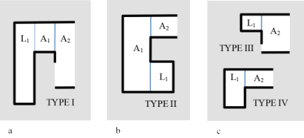
We call these subtrees Types I to IV. In Type I, $L_{1}$ and $A_{2}$ are tall neighbors of $A_{1}$, and they all share a horizontal edge. In Type II, $L_{1}$ and $A_{2}$ are paired neighbors of $A_{1}$. In Type III, the subtree of $A_{2}$ is a short leaf. In Type IV, the subtree of $A_{2}$ is a tall leaf.

We call Type II and Type IV subtrees tall, because they include a tall neighbor of $A_{2}$. We similarly call Type I and Type III subtrees short. Note that tall and short do not refer to the depth of the subtrees (Types I and II have depth 2, and Types III and IV have depth 1).

We now remove our assumption that $A_{2}$ is an upper-right neighbor of $A_{1}$ in order to assume (without loss of generality) that $A_{3}$ is an upper-right neighbor of $A_{2}$. Note that $A_{3}$ does exist because we have assumed that the depth of the dual tree is at least 3.

References

- [1] S. W. Bae, C. Shin, and A. Vigneron. Improved bounds for beacon-based coverage and routing in simple rectilinear polygons. arXiv:1505.05106, 2015.
- [2] M. Biro. Beacon-based routing and guarding. PhD thesis, State University of New York at Stony Brook, 2013.
- [3] M. Biro, J. Gao, J. Iwerks, I. Kostitsyna, and J. S. Mitchell. Combinatorics of beacon routing and coverage. In Proceedings of the 25th Canadian Conference on Computational Geometry, Waterloo, Ontario, 2013.
- [4] M. Biro, J. Iwerks, I. Kostitsyna, and J. S. Mitchell. Beacon-based algorithms for geometric routing. In F. Dehne, R. Solis-Oba, and J.-R. Sack, editors, Algorithms and Data Structures, pages 158–169. Springer, 2013.
- [5] P. Bose, P. Morin, I. Stojmenovic, and J. Urrutia. Routing with guaranteed delivery in ad hoc wireless networks. Wireless Networks, 7(6):609–616, 2001.
- [6] A. Fournier and D. Y. Montuno. Triangulating simple polygons and equivalent problems. ACM Transactions on Graphics (TOG), 3(2):153–174, 1984.
- [7] B. Karp and H. T. Kung. Gpsr: Greedy perimeter stateless routing for wireless networks. In Proceedings of the 6th Annual International Conference on Mobile Computing and Networking, MobiCom ’00, pages 243–254, New York, NY, USA, 2000. ACM.
- [8] A. Nguyen, N. Milosavljevic, Q. Fang, J. Gao, and L. Guibas. Landmark selection and greedy landmark-descent routing for sensor networks. In INFOCOM 2007. 26th IEEE International Conference on Computer Communications. IEEE, pages 661–669, May 2007.