跳到论文正文
W Papers独立论文阅读器 arXiv:1507.03470 论文正文 计算阅读时间 · 0%
引用这篇论文根据当前论文元数据生成,正式投稿前建议核对。


License: arXiv.org perpetual non-exclusive license
arXiv:1507.03470v2 [hep-ph] 10 Sep 2015

Renormalization group invariants in supersymmetric theories: one- and two-loop results

Wim Beenakker Affiliation: Institute for Mathematics, Astrophysics and Particle Physics, Faculty of Science, Mailbox 79, Radboud University Nijmegen, P.O. Box 9010, 6500 GL Nijmegen, The Netherlands Affiliation: Institute of Physics, University of Amsterdam, Science Park 904, 1018 XE Amsterdam, The Netherlands Email: W.Beenakker@science.ru.nl    Tom van Daal Affiliation: Department of Physics and Astronomy, VU University Amsterdam, De Boelelaan 1081, 1081 HV Amsterdam, The Netherlands Affiliation: Nikhef, Science Park 105, 1098 XG Amsterdam, The Netherlands Email: tvdaal@nikhef.nl    Ronald Kleiss Affiliation: Institute for Mathematics, Astrophysics and Particle Physics, Faculty of Science, Mailbox 79, Radboud University Nijmegen, P.O. Box 9010, 6500 GL Nijmegen, The Netherlands Email: R.Kleiss@science.ru.nl    Rob Verheyen Affiliation: Institute for Mathematics, Astrophysics and Particle Physics, Faculty of Science, Mailbox 79, Radboud University Nijmegen, P.O. Box 9010, 6500 GL Nijmegen, The Netherlands Email: robverheyen@gmail.com
Abstract

We stress the potential usefulness of renormalization group invariants. Especially particular combinations thereof could for instance be used as probes into patterns of supersymmetry breaking in the MSSM at inaccessibly high energies. We search for these renormalization group invariants in two systematic ways: on the one hand by making use of symmetry arguments and on the other by means of a completely automated exhaustive search through a large class of candidate invariants. At the one-loop level, we find all known invariants for the MSSM and in fact several more, and extend our results to the more constrained pMSSM and dMSSM, leading to even more invariants. Extending our search to the two-loop level we find that the number of invariants is considerably reduced.

Keywords
Renormalization Group, Supersymmetry, MSSM, pMSSM

1 Introduction

It has long been known that the Standard Model cannot be the final theory of particle physics. Issues such as the hierarchy problem or the absence of a satisfactory description of dark matter or gravity lead theoretical physicists to develop more fundamental theories. Supersymmetry is one of those theories, and the Minimal Supersymmetric Standard Model (MSSM) will be one of the main focuses for the second run of the Large Hadron Collider. If signs of supersymmetry are indeed found, theorists will face the issue of figuring out the exact underlying theoretical description. In case of the MSSM, this problem includes finding the exact mechanism of supersymmetry breaking. If supersymmetry is a symmetry of nature, every particle must have the same mass as its superpartner. Since this is clearly not the case, supersymmetry must be broken. The MSSM accounts for several breaking mechanisms by incorporating all possible soft supersymmetry breaking terms in its Lagrangian. If any of the several possible breaking mechanisms is realized in nature, this will be signified by a characteristic unification of some soft supersymmetry breaking parameters at a high energy scale.

These unifications can be studied through renormalization group (RG) techniques. Typical strategies include evolving the values of measured parameters upward to the unification scale (bottom-up), or choosing values of the parameters at the unification scale that are evolved downward (top-down). We will discuss a third method that makes use of RG invariant combinations of RG equations, called RG invariants. Using RG invariants to probe high-scale physics, has several distinct advantages over the bottom-up and top-down methods [1, 2, 3]. Finding these invariants can be very difficult though. In this paper we will discuss two different methods to find RG invariants. One method relates invariants to symmetries of the underlying theory and the other is based on computer algebraic techniques. Both methods will be applied to the MSSM, the diagonal MSSM (dMSSM), and the phenomenological MSSM (pMSSM) to find invariants up to two-loop order.

The paper is organized as follows. In section 2 we describe the method of RG invariants and its merits. In section 3 we investigate whether some of these RG invariants can be related to symmetries of the underlying theory. For this underlying theory we will consider the MSSM, dMSSM, and pMSSM. In section 4 a generic computer algebraic method for finding RG invariants is introduced. This method is used to find previously unknown invariants at one- and two-loop level within the aforementioned supersymmetric theories.

2 Probing high-scale physics with RG invariants

Let us consider a renormalized theory with a running parameter p⁡(μ)p(\mu). We define the corresponding β\beta-function as follows:

β⁡(p)≡16​π2​d​pd​t,\beta(p)\equiv 16\pi^{2}\frac{dp}{dt}, (1)

where t≡log10⁡(μ/μ0)t\equiv\log_{10}(\mu/\mu_{0}). The energy scale μ\mu is normalized by an arbitrary reference scale μ0\mu_{0} to make the logarithm dimensionless. For quantum field theories, the one-loop β\beta-functions are polynomials of the parameters of the theory with rational coefficients. Higher order contributions contain additional factors of 1/(16​π2)1/(16\pi^{2}).

How could RG invariants be used to probe high-scale physics? We will explain this through a toy system of one-loop β\beta-functions for the parameters v,w,x,y,zv,w,x,y,z that closely resembles some of the one-loop MSSM β\beta-functions; we define

β⁡(v)\displaystyle\beta(v) =v3,\displaystyle=v^{3}, (2a)
β⁡(w)\displaystyle\beta(w) =v2​(5​w+6​x−4​y),\displaystyle=v^{2}\left(5w+6x-4y\right), (2b)
β⁡(x)\displaystyle\beta(x) =v2​(−w−2​x+4​z),\displaystyle=v^{2}\left(-w-2x+4z\right), (2c)
β⁡(y)\displaystyle\beta(y) =v2​(x+y−5​z),\displaystyle=v^{2}\left(x+y-5z\right), (2d)
β⁡(z)\displaystyle\beta(z) =v2​(w−2​y+6​z).\displaystyle=v^{2}\left(w-2y+6z\right). (2e)

This system of β\beta-functions was built such that the parameter vv resembles a gauge coupling parameter, while w,x,y,zw,x,y,z resemble MSSM scalar masses. An RG invariant is an algebraic combination of parameters II, such that

dd​t​I=0.\frac{d}{dt}I=0. (3)

As it turns out, two independent RG invariants can be constructed from the β\beta-functions given by eqs. (2a) - (2e); we define

I1≡w+3​x−2​z,I2≡x+2​y+z.I_{1}\equiv w+3x-2z,\quad I_{2}\equiv x+2y+z. (4)

Supersymmetry breaking mechanisms typically predict the unification of scalar masses at some large, experimentally inaccessible energy scale. We can use the invariants in (4) to check whether the unification of w,x,y,zw,x,y,z is realized in nature. Suppose that these scalar masses unify to the value ss at some scale, then we would have

I1=2​s,I2=4​s,I_{1}=2s,\quad I_{2}=4s, (5)

from which it follows that

2​I1−I2=0.2I_{1}-I_{2}=0. (6)

Such a relation between RG invariants is called a sum rule. Since I1I_{1} and I2I_{2} are invariant under RG flow, sum rules such as eq. (6) remain true at all energy scales, if unification occurs. In particular, sum rules can be checked at the collider scale, potentially falsifying the assumed unification.

The approach using RG invariants avoids a number of issues that the top-down and bottom-up methods suffer from. The top-down method requires knowledge of both the unification scale and value in order to evolve the parameters down to experimentally accessible scales. Since theory does not predict these values with much accuracy, scans are typically performed over a range of scales and values. These scans can be computationally very time-consuming (depending on the number of unifying parameters), and are often not feasible. The use of RG invariants requires no knowledge of the unification scale or value whatsoever, so that this problem is avoided.

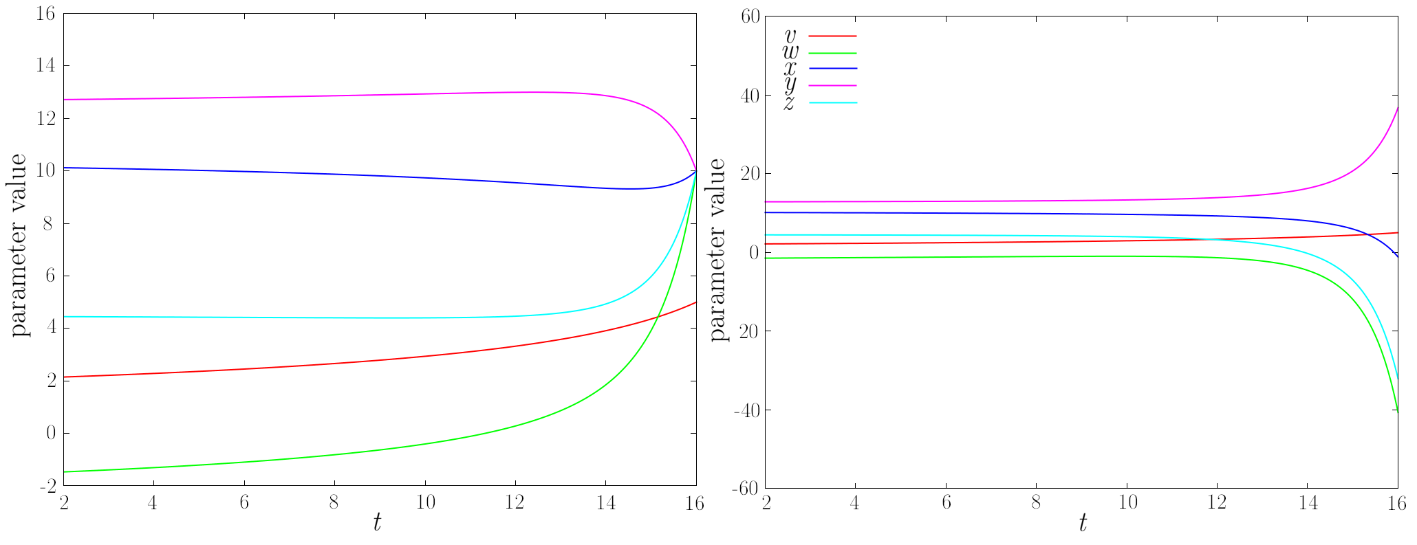
The bottom-up method does not require knowledge of unifying scales or values either, but suffers from a different problem resulting from the numerical evolution of experimental input values. When parameters are evolved up to higher scales, any experimental errors are typically greatly enhanced. Figure 1 shows the running effects of a slight change of one of the low-scale values of the parameters v,w,x,y,zv,w,x,y,z when w,x,y,zw,x,y,z unify at some high scale. After the slight change, the evolution of the parameters no longer shows any sign of unification whatsoever. The use of RG invariants circumvents such numerical problems.
Refer to caption
Figure 1: Left: The evolution of the parameters v,w,x,y,zv,w,x,y,z according to their one-loop β\beta-functions (2a) - (2e). The parameters w,x,y,zw,x,y,z unify at t=16t=16 to the value 1010. Right: The initial value of yy at t=2t=2 is raised by 1%1\%.

Finally, it is usually not necessary to know all parameters of the theory when using RG-invariants as probes of high-scale physics. The β\beta-functions for most theories are heavily coupled differential equations, and hence evolving the relevant parameters of a theory usually requires the evolution of all other parameters of the theory as well. In our example the sum rule of eq. (6) does not involve the parameter vv, which does not participate in the unification anyway. Both the top-down and bottom-up methods also require a value for vv to numerically evolve the other parameters.

Constructing RG invariants is generally a very non-trivial matter. To find invariants, we will not use the “standard” algebraical techniques that are used in for example [3]. Instead, we will consider two different, more efficient methods: one relies on symmetries of the underlying theory, and the other is based on computer algebraic techniques. Both methods will be applied to find invariants for the MSSM, the dMSSM, and the pMSSM.

3 RG invariants from symmetries

First, we will look at the construction of RG invariants from a perspective that involves symmetries of the underlying theory. The existence of such a relation between symmetries and invariants was suggested by [2] in the context of the pMSSM. As yet, no compelling arguments or proof of this has been presented though. First we will consider the MSSM, then we will study a “flavor-diagonal” version of the MSSM (the dMSSM), and, finally, the pMSSM will be discussed. All nomenclature regarding MSSM, dMSSM, and pMSSM fields and parameters is defined in appendices A, B, and C respectively.

3.1 The MSSM

In this subsection we attempt to construct RG invariants in the MSSM. So far, RG invariants have only been constructed for heavily constrained supersymmetric models, such as the pMSSM [2, 3]. We will attempt to construct invariants for the full 168-parameter MSSM.

3.1.1 Known invariants

We expect that some invariants that have been found in the pMSSM also exist in the MSSM, since the simplifications of the pMSSM with respect to the MSSM mainly apply to the family sector, and, for example, not at all to the gauge sector. The following invariants that have been found in the pMSSM are also invariants in the MSSM, which can be checked easily with the β\beta-functions in appendix A.4. In the combined gauge and gaugino sectors, we can construct three invariants:11 1 Strictly speaking there are six invariants: these three, plus their complex conjugates.

I1≡M1g′2,I2≡M2g2,I3≡M3gs2,I_{1}\equiv\frac{M_{1}}{g^{\prime 2}},\quad I_{2}\equiv\frac{M_{2}}{g^{2}},\quad I_{3}\equiv\frac{M_{3}}{g_{\text{s}}^{2}}, (7)

and in the pure gauge sector we have

I4≡1g′2−11g2,I5≡3g′2+11gs2.I_{4}\equiv\frac{1}{g^{\prime 2}}-\frac{11}{g^{2}},\quad I_{5}\equiv\frac{3}{g^{\prime 2}}+\frac{11}{g_{\text{s}}^{2}}. (8)

Finally, the invariant that involves the quantity SS turns out to be an invariant of the MSSM as well:

I6≡Sg′2.I_{6}\equiv\frac{S}{g^{\prime 2}}. (9)

Thus, six invariants that we already know from the pMSSM carry over trivially to the MSSM.

3.1.2 New invariants

As we know from [2, 3], all remaining invariants in the pMSSM (there exist eight more besides I1,…,I6I_{1},\ldots,I_{6}) involve scalar masses only, or combinations of scalar and gaugino masses.22 2 Actually, in the pMSSM two more invariants exist that involve the Higgs mixing parameters μ\mu and bb, but as argued in [3] these are useless to probe high-scale physics models. For completeness, though, they are listed in appendix D. For this reason, we will now focus on these sectors in the MSSM to see if more invariant quantities can be constructed.

Let us now try to construct invariants from the one-loop β\beta-functions of the soft scalar masses and gaugino masses that are listed in appendix A.4. The first thing we note when we look at the β\beta-functions for the soft scalar masses, is that no invariants can possibly be constructed for the off-diagonal terms of the sfermion mass matrices. The reason for this is that the order in which the family space matrices (i.e. the Yukawa and trilinear coupling matrices) appear is different for all five β\beta-functions of the sfermion mass matrices. In other words, there are simply too many different structures present. In order to avoid this, we need to work with terms that are insensitive to this order of matrices. Hence, a logical step would be to consider the β\beta-functions for the traces of the sfermion mass matrices. These β\beta-functions are given by

β⁡[Tr​(𝒎𝑸~𝟐)]=\displaystyle\beta\left[\text{Tr}(\boldsymbol{m_{\widetilde{Q}}^{2}})\right]= −24​YQ~L2​g′2​|M1|2−18​g2​|M2|2−32​gs2​|M3|2+6​YQ~L​g′2​S\displaystyle-24Y_{\widetilde{Q}_{L}}^{2}g^{\prime 2}|M_{1}|^{2}-18g^{2}|M_{2}|^{2}-32g_{\text{s}}^{2}|M_{3}|^{2}+6Y_{\widetilde{Q}_{L}}g^{\prime 2}S
+2​Tr​(mHu2​𝒚𝒖†​𝒚𝒖+𝒎𝑸~𝟐​𝒚𝒖†​𝒚𝒖+𝒚𝒖†​𝒎𝒖~𝟐​𝒚𝒖+𝒂𝒖†​𝒂𝒖)\displaystyle+2\,\text{Tr}\left(m_{H_{u}}^{2}\boldsymbol{y_{u}^{\dagger}y_{u}}+\boldsymbol{m_{\widetilde{Q}}^{2}y_{u}^{\dagger}y_{u}}+\boldsymbol{y_{u}^{\dagger}m_{\widetilde{u}}^{2}y_{u}}+\boldsymbol{a_{u}^{\dagger}a_{u}}\right)
+2​Tr​(mHd2​𝒚𝒅†​𝒚𝒅+𝒎𝑸~𝟐​𝒚𝒅†​𝒚𝒅+𝒚𝒅†​𝒎𝒅~𝟐​𝒚𝒅+𝒂𝒅†​𝒂𝒅),\displaystyle+2\,\text{Tr}\left(m_{H_{d}}^{2}\boldsymbol{y_{d}^{\dagger}y_{d}}+\boldsymbol{m_{\widetilde{Q}}^{2}y_{d}^{\dagger}y_{d}}+\boldsymbol{y_{d}^{\dagger}m_{\widetilde{d}}^{2}y_{d}}+\boldsymbol{a_{d}^{\dagger}a_{d}}\right), (10a)
β⁡[Tr​(𝒎𝑳~𝟐)]=\displaystyle\beta\left[\text{Tr}(\boldsymbol{m_{\widetilde{L}}^{2}})\right]= −24​YL~L2​g′2​|M1|2−18​g2​|M2|2+6​YL~L​g′2​S\displaystyle-24Y_{\widetilde{L}_{L}}^{2}g^{\prime 2}|M_{1}|^{2}-18g^{2}|M_{2}|^{2}+6Y_{\widetilde{L}_{L}}g^{\prime 2}S
+2​Tr​(mHd2​𝒚𝒆†​𝒚𝒆+𝒎𝑳~𝟐​𝒚𝒆†​𝒚𝒆+𝒚𝒆†​𝒎𝒆~𝟐​𝒚𝒆+𝒂𝒆†​𝒂𝒆),\displaystyle+2\,\text{Tr}\left(m_{H_{d}}^{2}\boldsymbol{y_{e}^{\dagger}y_{e}}+\boldsymbol{m_{\widetilde{L}}^{2}y_{e}^{\dagger}y_{e}}+\boldsymbol{y_{e}^{\dagger}m_{\widetilde{e}}^{2}y_{e}}+\boldsymbol{a_{e}^{\dagger}a_{e}}\right), (10b)
β⁡[Tr​(𝒎𝒖~𝟐)]=\displaystyle\beta\left[\text{Tr}(\boldsymbol{m_{\widetilde{u}}^{2}})\right]= −24​Yu~R∗2​g′2​|M1|2−32​gs2​|M3|2+6​Yu~R∗​g′2​S\displaystyle-24Y_{\widetilde{u}_{R}^{*}}^{2}g^{\prime 2}|M_{1}|^{2}-32g_{\text{s}}^{2}|M_{3}|^{2}+6Y_{\widetilde{u}_{R}^{*}}g^{\prime 2}S
+4​Tr​(mHu2​𝒚𝒖†​𝒚𝒖+𝒎𝑸~𝟐​𝒚𝒖†​𝒚𝒖+𝒚𝒖†​𝒎𝒖~𝟐​𝒚𝒖+𝒂𝒖†​𝒂𝒖),\displaystyle+4\,\text{Tr}\left(m_{H_{u}}^{2}\boldsymbol{y_{u}^{\dagger}y_{u}}+\boldsymbol{m_{\widetilde{Q}}^{2}y_{u}^{\dagger}y_{u}}+\boldsymbol{y_{u}^{\dagger}m_{\widetilde{u}}^{2}y_{u}}+\boldsymbol{a_{u}^{\dagger}a_{u}}\right), (10c)
β⁡[Tr​(𝒎𝒅~𝟐)]=\displaystyle\beta\left[\text{Tr}(\boldsymbol{m_{\widetilde{d}}^{2}})\right]= −24​Yd~R∗2​g′2​|M1|2−32​gs2​|M3|2+6​Yd~R∗​g′2​S\displaystyle-24Y_{\widetilde{d}_{R}^{*}}^{2}g^{\prime 2}|M_{1}|^{2}-32g_{\text{s}}^{2}|M_{3}|^{2}+6Y_{\widetilde{d}_{R}^{*}}g^{\prime 2}S
+4​Tr​(mHd2​𝒚𝒅†​𝒚𝒅+𝒎𝑸~𝟐​𝒚𝒅†​𝒚𝒅+𝒚𝒅†​𝒎𝒅~𝟐​𝒚𝒅+𝒂𝒅†​𝒂𝒅),\displaystyle+4\,\text{Tr}\left(m_{H_{d}}^{2}\boldsymbol{y_{d}^{\dagger}y_{d}}+\boldsymbol{m_{\widetilde{Q}}^{2}y_{d}^{\dagger}y_{d}}+\boldsymbol{y_{d}^{\dagger}m_{\widetilde{d}}^{2}y_{d}}+\boldsymbol{a_{d}^{\dagger}a_{d}}\right), (10d)
β⁡[Tr​(𝒎𝒆~𝟐)]=\displaystyle\beta\left[\text{Tr}(\boldsymbol{m_{\widetilde{e}}^{2}})\right]= −24​Ye~R∗2​g′2​|M1|2+6​Ye~R∗​g′2​S\displaystyle-24Y_{\widetilde{e}_{R}^{*}}^{2}g^{\prime 2}|M_{1}|^{2}+6Y_{\widetilde{e}_{R}^{*}}g^{\prime 2}S
+4​Tr​(mHd2​𝒚𝒆†​𝒚𝒆+𝒎𝑳~𝟐​𝒚𝒆†​𝒚𝒆+𝒚𝒆†​𝒎𝒆~𝟐​𝒚𝒆+𝒂𝒆†​𝒂𝒆),\displaystyle+4\,\text{Tr}\left(m_{H_{d}}^{2}\boldsymbol{y_{e}^{\dagger}y_{e}}+\boldsymbol{m_{\widetilde{L}}^{2}y_{e}^{\dagger}y_{e}}+\boldsymbol{y_{e}^{\dagger}m_{\widetilde{e}}^{2}y_{e}}+\boldsymbol{a_{e}^{\dagger}a_{e}}\right), (10e)
β⁡(mHu2)=\displaystyle\beta(m_{H_{u}}^{2})= −8​YHu2​g′2​|M1|2−6​g2​|M2|2+2​YHu​g′2​S\displaystyle-8Y_{H_{u}}^{2}g^{\prime 2}|M_{1}|^{2}-6g^{2}|M_{2}|^{2}+2Y_{H_{u}}g^{\prime 2}S
+6​Tr​(mHu2​𝒚𝒖†​𝒚𝒖+𝒎𝑸~𝟐​𝒚𝒖†​𝒚𝒖+𝒚𝒖†​𝒎𝒖~𝟐​𝒚𝒖+𝒂𝒖†​𝒂𝒖),\displaystyle+6\,\text{Tr}\left(m_{H_{u}}^{2}\boldsymbol{y_{u}^{\dagger}y_{u}}+\boldsymbol{m_{\widetilde{Q}}^{2}y_{u}^{\dagger}y_{u}}+\boldsymbol{y_{u}^{\dagger}m_{\widetilde{u}}^{2}y_{u}}+\boldsymbol{a_{u}^{\dagger}a_{u}}\right), (10f)
β⁡(mHd2)=\displaystyle\beta(m_{H_{d}}^{2})= −8​YHd2​g′2​|M1|2−6​g2​|M2|2+2​YHd​g′2​S\displaystyle-8Y_{H_{d}}^{2}g^{\prime 2}|M_{1}|^{2}-6g^{2}|M_{2}|^{2}+2Y_{H_{d}}g^{\prime 2}S
+6​Tr​(mHd2​𝒚𝒅†​𝒚𝒅+𝒎𝑸~𝟐​𝒚𝒅†​𝒚𝒅+𝒚𝒅†​𝒎𝒅~𝟐​𝒚𝒅+𝒂𝒅†​𝒂𝒅)\displaystyle+6\,\text{Tr}\left(m_{H_{d}}^{2}\boldsymbol{y_{d}^{\dagger}y_{d}}+\boldsymbol{m_{\widetilde{Q}}^{2}y_{d}^{\dagger}y_{d}}+\boldsymbol{y_{d}^{\dagger}m_{\widetilde{d}}^{2}y_{d}}+\boldsymbol{a_{d}^{\dagger}a_{d}}\right)
+2​Tr​(mHd2​𝒚𝒆†​𝒚𝒆+𝒎𝑳~𝟐​𝒚𝒆†​𝒚𝒆+𝒚𝒆†​𝒎𝒆~𝟐​𝒚𝒆+𝒂𝒆†​𝒂𝒆),\displaystyle+2\,\text{Tr}\left(m_{H_{d}}^{2}\boldsymbol{y_{e}^{\dagger}y_{e}}+\boldsymbol{m_{\widetilde{L}}^{2}y_{e}^{\dagger}y_{e}}+\boldsymbol{y_{e}^{\dagger}m_{\widetilde{e}}^{2}y_{e}}+\boldsymbol{a_{e}^{\dagger}a_{e}}\right), (10g)

where, for convenience, we have also added the β\beta-functions for mHu2m_{H_{u}}^{2} and mHd2m_{H_{d}}^{2} (which already involved traces).

In the MSSM, all interactions in family space are described by the Yukawa terms in the superpotential and the soft supersymmetry breaking trilinear terms (cf. appendix A.2). In case that the order of the family space matrices does not matter by taking a trace, then these interactions give rise to three different trace structures in (10a) - (10g), labeled by u,d,u,d, and ee. These trace structures each belong to one of the three Yukawa and trilinear interaction terms in the superpotential and the soft breaking Lagrangian respectively, and each of those terms involves a unique set of three scalar fields. For example, the terms in the MSSM Lagrangian that give rise to the trace structure that features the label uu are

Δ​WMSSM=u~R†​𝒚𝒖​(Q~L)α​(Hu)α,Δ​ℒtril.=−u~R†​𝒂𝒖​(Q~L)α​(Hu)α+h.c.\Delta W_{\text{MSSM}}=\widetilde{u}_{R}^{\dagger}\boldsymbol{y_{u}}(\widetilde{Q}_{L})^{\alpha}(H_{u})_{\alpha},\quad\Delta\mathscr{L}_{\text{tril.}}=-\widetilde{u}_{R}^{\dagger}\boldsymbol{a_{u}}(\widetilde{Q}_{L})^{\alpha}(H_{u})_{\alpha}+\text{h.c.} (11)

Note that the coefficients of the three trace structures are different for the various scalar masses. This is because in the β\beta-functions no traces have been carried out over the gauge degrees of freedom of the corresponding scalar fields. How is this to be understood? Let us consider the trilinear interaction between the fields u~R\widetilde{u}_{R}, Q~L\widetilde{Q}_{L}, and HuH_{u}, as well as the one-loop corrections to the scalar propagators that this interaction gives rise to. These three fields can all occur as external fields or inside loops. The gauge degrees of freedom that are “closed” inside the loops (i.e. those gauge degrees of freedom that the external fields do not possess) are summed over. Say we take u~R\widetilde{u}_{R} to be the external field, then there is an SU​(2)\text{SU}(2) doublet degree of freedom inside the loop that has to be “traced over”, giving a factor of 2. If we had taken HuH_{u} to be the external field, then a trace over SU​(3)\text{SU}(3) degrees of freedom inside the loop would have resulted, giving a factor of 3, etc. Hence, if we multiply the β\beta-functions (10a) - (10g) by the factors that result from summing over the gauge degrees of freedom of the external scalar fields, then all three trace structures each get exactly the same coefficients.

How many RG invariants do we expect to find in the soft scalar and gaugino sectors? We have ten equations (seven β\beta-functions for the scalar masses and three for the gaugino masses) that contain seven different structures (three trace structures, three gaugino masses and SS). Having ten equations to eliminate seven different terms should give 10−7=310-7=3 independent RG invariants.

To construct invariant quantities from these β\beta-functions, we can first try to get rid of the three different trace structures. To cancel these structures, we could consider a linear sum of the β\beta-functions (10a) - (10g), appropriately multiplied by numbers of gauge degrees of freedom, such that the coefficients of this sum add up to zero for each trace structure. Now we can use the fact that each trace structure corresponds to a unique combination of three scalar fields in the Lagrangian. For the cancellation to take place, we should assign quantum numbers to these groups of three fields that each add up to zero, which is equivalent to saying that the quantum number should be conserved by all family space interactions. This means that to cancel the Yukawa and trilinear contributions to the β\beta-functions, we should consider U​(1)\text{U}(1) symmetries of the MSSM family sector. More specifically, for any quantum number QQ that pertains to a symmetry U​(1)Q\text{U}(1)_{Q} of the MSSM family sector, the β\beta-function of the quantity

Tr​(∑ϕQϕ​𝒎ϕ𝟐),\text{Tr}\bigg(\sum_{\phi}Q_{\phi}\boldsymbol{m_{\phi}^{2}}\bigg), (12)

with the sum running over all scalar fields ϕ\phi, does no longer contain the three trace structures. Note that sums like the one in (12) over fields that occur inside family space traces are implicitly understood to be over all gauge degrees of freedom of the gauge multiplets.33 3 For the field Q~L\widetilde{Q}_{L}, for example, such a sum would give a factor of 2 for SU​(2)\text{SU}(2) and a factor of 3 for SU​(3)\text{SU}(3) degrees of freedom, yielding a total multiplication by 6.

What could the quantum number QQ be? As is discussed in appendix A.3, the relevant U​(1)\text{U}(1) symmetries correspond to the quantum numbers weak hypercharge (YY), baryon number (BB), lepton number (LL), and XX. Table 1 provides the quantum numbers Y,B,L,XY,B,L,X for all scalar fields in the MSSM. The presence of exactly four independent U​(1)\text{U}(1) symmetries in the family sector of the MSSM can be explained as follows: from table 1 we infer that this sector of the theory is constituted by seven scalar multiplets. We can regard each set of quantum numbers pertaining to a given symmetry as being a vector in a seven-dimensional vector space. This vector is subject to three independent symmetry constraints coming from the interaction terms in the superpotential and the soft trilinear terms (the terms in eq. (11) give one of these constraints). This means that we can construct 7−3=47-3=4 linearly independent vectors in this space, i.e. four sets of quantum numbers each corresponding to a different U​(1)\text{U}(1) symmetry.

Spin 0 𝒀\boldsymbol{Y} 𝑩\boldsymbol{B} 𝑳\boldsymbol{L} 𝑿\boldsymbol{X}
Q~L\widetilde{Q}_{L} 16\frac{1}{6} 13\frac{1}{3} 00 11
L~L\widetilde{L}_{L} −12-\frac{1}{2} 00 11 11
u~R∗\widetilde{u}_{R}^{*} −23-\frac{2}{3} −13-\frac{1}{3} 00 11
d~R∗\widetilde{d}_{R}^{*} 13\frac{1}{3} −13-\frac{1}{3} 00 11
e~R∗\widetilde{e}_{R}^{*} 11 00 −1-1 11
HuH_{u} 12\frac{1}{2} 00 00 −2-2
HdH_{d} −12-\frac{1}{2} 00 00 −2-2
Table 1: The quantum numbers Y,B,L,XY,B,L,X for all MSSM scalar fields.

We now know how to get rid of the three family space trace structures in eqs. (10a) - (10g), but what about the other terms present? Can quantum numbers also be used to eliminate the remaining structures (i.e. SS and the three absolute squared gaugino masses |M1|2,|M2|2,|M3|2|M_{1}|^{2},|M_{2}|^{2},|M_{3}|^{2})? For any QQ, we have

β⁡[Tr​(∑ϕQϕ​𝒎ϕ𝟐)]=\displaystyle\beta\bigg[\text{Tr}\bigg(\sum_{\phi}Q_{\phi}\boldsymbol{m_{\phi}^{2}}\bigg)\bigg]=  2​(∑ϕYϕ​Qϕ)​g′2​S−8​(∑ϕYϕ2​Qϕ)​g′2​|M1|2\displaystyle\;2\bigg(\sum_{\phi}Y_{\phi}Q_{\phi}\bigg)g^{\prime 2}S-8\bigg(\sum_{\phi}Y_{\phi}^{2}Q_{\phi}\bigg)g^{\prime 2}|M_{1}|^{2}
−6​(∑dQd)​g2​|M2|2−323​(∑tQt)​gs2​|M3|2,\displaystyle-6\bigg(\sum_{d}Q_{d}\bigg)g^{2}|M_{2}|^{2}-\frac{32}{3}\bigg(\sum_{t}Q_{t}\bigg)g_{\text{s}}^{2}|M_{3}|^{2}, (13)

where dd denotes the scalar weak isospin doublets and tt the scalar color triplets. Note that sums without any family space traces involved are implicitly understood to be over all families as well (besides the gauge degrees of freedom).44 4 This simply amounts to an additional factor of 33 for all sfermions. From eq. (13) it directly follows that to eliminate S,|M1|2,|M2|2,|M3|2S,|M_{1}|^{2},|M_{2}|^{2},|M_{3}|^{2} respectively, we must have:

∑ϕYϕ​Qϕ=0,∑ϕYϕ2​Qϕ=0,∑dQd=0,∑tQt=0.\sum_{\phi}Y_{\phi}Q_{\phi}=0,\quad\sum_{\phi}Y_{\phi}^{2}Q_{\phi}=0,\quad\sum_{d}Q_{d}=0,\quad\sum_{t}Q_{t}=0. (14)

The latter three sums over charges are reminiscent of mixed anomaly cancellations of the charge QQ with the separate gauge groups that we know from for example the Standard Model.

Which quantum numbers actually satisfy the requirements in (14)? This is summarized in table 2. From this table it follows that to eliminate SS, suitable quantum numbers would be 3​B+L3B+L, 11​(B−L)−8​Y11(B-L)-8Y, and XX. For the cancellation of |M1|2|M_{1}|^{2}, we could use YY, B−LB-L, or 16​B+3​X16B+3X, while for |M2|2|M_{2}|^{2} the quantum numbers YY, B−LB-L, and 8​B−3​X8B-3X are suitable. For |M3|2|M_{3}|^{2} to cancel, we could pick YY, BB, or LL. Naturally, linear combinations of these quantum numbers also work.

Quantity Sum 𝒀\boldsymbol{Y} 𝑩\boldsymbol{B} 𝑳\boldsymbol{L} 𝑿\boldsymbol{X}
SS ∑ϕYϕ​Qϕ\sum_{\phi}Y_{\phi}Q_{\phi} 1111 22 −6-6 00
|M1|2|M_{1}|^{2} ∑ϕYϕ2​Qϕ\sum_{\phi}Y_{\phi}^{2}Q_{\phi} 00 −32-\frac{3}{2} −32-\frac{3}{2} 88
|M2|2|M_{2}|^{2} ∑dQd\sum_{d}Q_{d} 00 66 66 1616
|M3|2|M_{3}|^{2} ∑tQt\sum_{t}Q_{t} 00 00 00 3636
Table 2: The evaluation of the sums that are related to the elimination requirements (14) for the quantities SS, |M1,2,3|2|M_{1,2,3}|^{2}, given for the quantum numbers Y,B,L,XY,B,L,X. The outcome 00 for a certain quantum number indicates that this quantum number is suitable for eliminating the corresponding quantity from the β\beta-functions (10a) - (10g).

From eq. (13), as well as from the β\beta-functions for the gaugino masses (66) and SS (69), it follows that any one-loop RG invariant II in the MSSM that involves scalar masses and gaugino masses, is of the following form:

IQ=\displaystyle I_{Q}= Tr​(∑ϕQϕ​𝒎ϕ𝟐)−111​∑ϕYϕ​Qϕ​S+211​∑ϕYϕ2​Qϕ​|M1|2+32​∑dQd​|M2|2\displaystyle\;\text{Tr}\bigg(\sum_{\phi}Q_{\phi}\boldsymbol{m_{\phi}^{2}}\bigg)-\frac{1}{11}\sum_{\phi}Y_{\phi}Q_{\phi}S+\frac{2}{11}\sum_{\phi}Y_{\phi}^{2}Q_{\phi}|M_{1}|^{2}+\frac{3}{2}\sum_{d}Q_{d}|M_{2}|^{2}
−89∑tQt|M3|2,\displaystyle-\frac{8}{9}\sum_{t}Q_{t}|M_{3}|^{2}, (15)

where QQ is any quantum number that is preserved by all MSSM family space interactions (i.e. QQ must be a linear combination of Y,B,L,XY,B,L,X).

Now we are ready to construct RG invariants using table 2 and eq. (15). From table 2 we infer that the quantum number 11​(B−L)−8​Y11(B-L)-8Y cancels SS and all gaugino masses, as this linear combination of Y,B,LY,B,L vanishes for each row in the table. This leads us to define the following RG invariant:

I7≡\displaystyle I_{7}\equiv Tr​(∑ϕ(11​Bϕ−11​Lϕ−8​Yϕ)​𝒎ϕ𝟐)\displaystyle\;\text{Tr}\bigg(\sum_{\phi}\left(11B_{\phi}-11L_{\phi}-8Y_{\phi}\right)\boldsymbol{m_{\phi}^{2}}\bigg)
=\displaystyle= Tr​(14​𝒎𝑸~𝟐−14​𝒎𝑳~𝟐+5​𝒎𝒖~𝟐−19​𝒎𝒅~𝟐+3​𝒎𝒆~𝟐)−8​mHu2+8​mHd2.\displaystyle\;\text{Tr}\left(14\boldsymbol{m_{\widetilde{Q}}^{2}}-14\boldsymbol{m_{\widetilde{L}}^{2}}+5\boldsymbol{m_{\widetilde{u}}^{2}}-19\boldsymbol{m_{\widetilde{d}}^{2}}+3\boldsymbol{m_{\widetilde{e}}^{2}}\right)-8m_{H_{u}}^{2}+8m_{H_{d}}^{2}. (16)

If we wish to construct an invariant where both SS and |M3|2|M_{3}|^{2} are eliminated by a symmetry, then we could use the quantum number 3​B+L3B+L. We define

I8≡\displaystyle I_{8}\equiv Tr​(∑ϕ(3​Bϕ+Lϕ)​𝒎ϕ𝟐)+211​∑ϕYϕ2​(3​Bϕ+Lϕ)​|M1|2+32​∑d(3​Bd+Ld)​|M2|2\displaystyle\;\text{Tr}\bigg(\sum_{\phi}(3B_{\phi}+L_{\phi})\boldsymbol{m_{\phi}^{2}}\bigg)+\frac{2}{11}\sum_{\phi}Y_{\phi}^{2}(3B_{\phi}+L_{\phi})|M_{1}|^{2}+\frac{3}{2}\sum_{d}(3B_{d}+L_{d})|M_{2}|^{2}
=\displaystyle= Tr​(6​𝒎𝑸~𝟐+2​𝒎𝑳~𝟐−3​𝒎𝒖~𝟐−3​𝒎𝒅~𝟐−𝒎𝒆~𝟐)−1211​|M1|2+36​|M2|2.\displaystyle\;\text{Tr}\left(6\boldsymbol{m_{\widetilde{Q}}^{2}}+2\boldsymbol{m_{\widetilde{L}}^{2}}-3\boldsymbol{m_{\widetilde{u}}^{2}}-3\boldsymbol{m_{\widetilde{d}}^{2}}-\boldsymbol{m_{\widetilde{e}}^{2}}\right)-\frac{12}{11}|M_{1}|^{2}+36|M_{2}|^{2}. (17)

For the third and last independent invariant in this sector, let us pick the quantum number XX (which only cancels SS) and define55 5 Even though we have four symmetries at hand, only three independent RG invariants can be constructed. This is because taking Q∝YQ\propto Y gives IQ=0I_{Q}=0. In fact, the quantum number YY has already been used for the invariant that involves the quantity SS (cf. eq. (9)).

I9≡\displaystyle I_{9}\equiv Tr​(∑ϕXϕ​𝒎ϕ𝟐)+211​∑ϕYϕ2​Xϕ​|M1|2+32​∑dXd​|M2|2−89​∑tXt​|M3|2\displaystyle\;\text{Tr}\bigg(\sum_{\phi}X_{\phi}\boldsymbol{m_{\phi}^{2}}\bigg)+\frac{2}{11}\sum_{\phi}Y_{\phi}^{2}X_{\phi}|M_{1}|^{2}+\frac{3}{2}\sum_{d}X_{d}|M_{2}|^{2}-\frac{8}{9}\sum_{t}X_{t}|M_{3}|^{2}
=\displaystyle= Tr​(6​𝒎𝑸~𝟐+2​𝒎𝑳~𝟐+3​𝒎𝒖~𝟐+3​𝒎𝒅~𝟐+𝒎𝒆~𝟐)−4​mHu2−4​mHd2+1611​|M1|2\displaystyle\;\text{Tr}\left(6\boldsymbol{m_{\widetilde{Q}}^{2}}+2\boldsymbol{m_{\widetilde{L}}^{2}}+3\boldsymbol{m_{\widetilde{u}}^{2}}+3\boldsymbol{m_{\widetilde{d}}^{2}}+\boldsymbol{m_{\widetilde{e}}^{2}}\right)-4m_{H_{u}}^{2}-4m_{H_{d}}^{2}+\frac{16}{11}|M_{1}|^{2}
+24​|M2|2−32​|M3|2.\displaystyle+24|M_{2}|^{2}-32|M_{3}|^{2}. (18)

3.2 The dMSSM

Let us consider a constrained version of the MSSM, the so-called dMSSM, where all matrices in family space (i.e. the sfermion mass matrices and the Yukawa and trilinear coupling matrices) are taken diagonal (cf. appendix B for a more extensive discussion of the dMSSM), and let us again focus on the soft scalar and gaugino sectors to find RG invariants. In this particular model, we have twenty equations (fifteen β\beta-functions for the sfermion masses, two for the Higgs masses, and three for the gaugino masses) containing thirteen different structures (nine structures coming from the diagonal components of the Yukawa and trilinear coupling matrices, three gaugino masses, and SS). Eliminating only thirteen different terms using twenty equations would result in 20−13=720-13=7 RG invariant quantities for this simplified model, on top of I1,…,I6I_{1},\ldots,I_{6}.

The “traced” β\beta-functions for this simplified model are again given by eqs. (10a) - (10g) and, as we discussed in the previous subsection, give rise to three independent RG invariants of the form (15). Thus, the invariants I7,I8,I9I_{7},I_{8},I_{9} are also invariants in this model. How can we construct the remaining four invariants? Can we again benefit from symmetry arguments?

As we have taken all family space matrices diagonal, there is no longer any flavor mixing present. In other words, the three (s)fermionic generations have completely decoupled. This means that the baryon and lepton numbers are separately conserved for each generation, i.e. BB and LL can now be split up into B1,B2,B3B_{1},B_{2},B_{3} and L1,L2,L3L_{1},L_{2},L_{3} respectively.66 6 Note that two linear combinations of these six quantum numbers are equivalent to BB and LL, namely the combinations B1+B2+B3B_{1}+B_{2}+B_{3} and L1+L2+L3L_{1}+L_{2}+L_{3} respectively. Table 3 provides all quantum numbers that pertain to (independent) U​(1)\text{U}(1) symmetries of the dMSSM. The completeness of this list can be shown in the same way as we did for the MSSM: from table 3 and appendix A.2 we infer that we have seventeen gauge multiplets that are subject to three constraints per generation. Hence there must be 17−3×3=817-3\times 3=8 independent U​(1)\text{U}(1) symmetries in this model.

Spin 0 𝒀\boldsymbol{Y} 𝑩𝟏\boldsymbol{B_{1}} 𝑩𝟐\boldsymbol{B_{2}} 𝑩𝟑\boldsymbol{B_{3}} 𝑳𝟏\boldsymbol{L_{1}} 𝑳𝟐\boldsymbol{L_{2}} 𝑳𝟑\boldsymbol{L_{3}} 𝑿\boldsymbol{X}
(Q~L)1(\widetilde{Q}_{L})_{1} 16\frac{1}{6} 13\frac{1}{3} 00 00 00 00 00 11
(Q~L)2(\widetilde{Q}_{L})_{2} 16\frac{1}{6} 00 13\frac{1}{3} 00 00 00 00 11
(Q~L)3(\widetilde{Q}_{L})_{3} 16\frac{1}{6} 00 00 13\frac{1}{3} 00 00 00 11
(L~L)1(\widetilde{L}_{L})_{1} −12-\frac{1}{2} 00 00 00 11 00 00 11
(L~L)2(\widetilde{L}_{L})_{2} −12-\frac{1}{2} 00 00 00 00 11 00 11
(L~L)3(\widetilde{L}_{L})_{3} −12-\frac{1}{2} 00 00 00 00 00 11 11
(u~R∗)1(\widetilde{u}_{R}^{*})_{1} −23-\frac{2}{3} −13-\frac{1}{3} 00 00 00 00 00 11
(u~R∗)2(\widetilde{u}_{R}^{*})_{2} −23-\frac{2}{3} 00 −13-\frac{1}{3} 00 00 00 00 11
(u~R∗)3(\widetilde{u}_{R}^{*})_{3} −23-\frac{2}{3} 00 00 −13-\frac{1}{3} 00 00 00 11
(d~R∗)1(\widetilde{d}_{R}^{*})_{1} 13\frac{1}{3} −13-\frac{1}{3} 00 00 00 00 00 11
(d~R∗)2(\widetilde{d}_{R}^{*})_{2} 13\frac{1}{3} 00 −13-\frac{1}{3} 00 00 00 00 11
(d~R∗)3(\widetilde{d}_{R}^{*})_{3} 13\frac{1}{3} 00 00 −13-\frac{1}{3} 00 00 00 11
(e~R∗)1(\widetilde{e}_{R}^{*})_{1} 11 00 00 00 −1-1 00 00 11
(e~R∗)2(\widetilde{e}_{R}^{*})_{2} 11 00 00 00 00 −1-1 00 11
(e~R∗)3(\widetilde{e}_{R}^{*})_{3} 11 00 00 00 00 00 −1-1 11
HuH_{u} 12\frac{1}{2} 00 00 00 00 00 00 −2-2
HdH_{d} −12-\frac{1}{2} 00 00 00 00 00 00 −2-2
Table 3: All quantum numbers that pertain to U​(1)\text{U}(1) symmetries of the dMSSM family sector. The dashed lines separate the different family multiplets.

Since there are four new independent symmetries in the dMSSM with respect to the MSSM, four additional invariants of the form

IQ=∑ϕQϕ​mϕ2−111​∑ϕYϕ​Qϕ​S+211​∑ϕYϕ2​Qϕ​|M1|2+32​∑dQd​|M2|2−89​∑tQt​|M3|2I_{Q}=\sum_{\phi}Q_{\phi}m_{\phi}^{2}-\frac{1}{11}\sum_{\phi}Y_{\phi}Q_{\phi}S+\frac{2}{11}\sum_{\phi}Y_{\phi}^{2}Q_{\phi}|M_{1}|^{2}+\frac{3}{2}\sum_{d}Q_{d}|M_{2}|^{2}-\frac{8}{9}\sum_{t}Q_{t}|M_{3}|^{2} (19)

can be constructed. Clearly, the quantum numbers B1−B2B_{1}-B_{2}, B1−B3B_{1}-B_{3}, L1−L2L_{1}-L_{2}, and L1−L3L_{1}-L_{3} automatically eliminate both SS and all gaugino masses. We define

I10≡\displaystyle I_{10}\equiv ∑ϕ(B1ϕ−B2ϕ)​mϕ2=2​mQ~12−mu~12−md~12−2​mQ~22+mu~22+md~22,\displaystyle\,\sum_{\phi}({B_{1}}_{\phi}-{B_{2}}_{\phi})m_{\phi}^{2}=2m_{\widetilde{Q}_{1}}^{2}-m_{\widetilde{u}_{1}}^{2}-m_{\widetilde{d}_{1}}^{2}-2m_{\widetilde{Q}_{2}}^{2}+m_{\widetilde{u}_{2}}^{2}+m_{\widetilde{d}_{2}}^{2}, (20a)
I11≡\displaystyle I_{11}\equiv ∑ϕ(B1ϕ−B3ϕ)​mϕ2=2​mQ~12−mu~12−md~12−2​mQ~32+mu~32+md~32,\displaystyle\,\sum_{\phi}({B_{1}}_{\phi}-{B_{3}}_{\phi})m_{\phi}^{2}=2m_{\widetilde{Q}_{1}}^{2}-m_{\widetilde{u}_{1}}^{2}-m_{\widetilde{d}_{1}}^{2}-2m_{\widetilde{Q}_{3}}^{2}+m_{\widetilde{u}_{3}}^{2}+m_{\widetilde{d}_{3}}^{2}, (20b)
I12≡\displaystyle I_{12}\equiv ∑ϕ(L1ϕ−L2ϕ)​mϕ2=2​mL~12−me~12−2​mL~22+me~22,\displaystyle\,\sum_{\phi}({L_{1}}_{\phi}-{L_{2}}_{\phi})m_{\phi}^{2}=2m_{\widetilde{L}_{1}}^{2}-m_{\widetilde{e}_{1}}^{2}-2m_{\widetilde{L}_{2}}^{2}+m_{\widetilde{e}_{2}}^{2}, (20c)
I13≡\displaystyle I_{13}\equiv ∑ϕ(L1ϕ−L3ϕ)​mϕ2=2​mL~12−me~12−2​mL~32+me~32.\displaystyle\,\sum_{\phi}({L_{1}}_{\phi}-{L_{3}}_{\phi})m_{\phi}^{2}=2m_{\widetilde{L}_{1}}^{2}-m_{\widetilde{e}_{1}}^{2}-2m_{\widetilde{L}_{3}}^{2}+m_{\widetilde{e}_{3}}^{2}. (20d)

3.3 The pMSSM

For the pMSSM, with respect to the dMSSM, there are a couple of additional constraints: the first two generations of sfermions are mass degenerate, and the Yukawa and trilinear coupling matrices only have non-zero entries for the third generation sfermions (cf. appendix C for a more extensive discussion of the pMSSM). This means that for the pMSSM we have fifteen equations (ten β\beta-functions for the sfermion masses, two for the Higgs masses, and three for the gaugino masses) to eliminate seven different structures (three structures coming from the (33)-components of the Yukawa and trilinear coupling matrices, three gaugino masses, and SS), which should yield 15−7=815-7=8 invariant quantities on top of I1,…,I6I_{1},\ldots,I_{6}. Indeed, for the pMSSM eight RG invariant quantities have been constructed in [2, 3] that involve scalar and gaugino masses only. Can we construct these invariants also based on our approach involving symmetries?

Again, three independent invariants can be constructed that are of the form (15), thus I7,I8,I9I_{7},I_{8},I_{9} trivially carry over to the pMSSM. Of the invariants I10,…,I13I_{10},\ldots,I_{13}, only I11I_{11} and I13I_{13} also exist in the pMSSM (the invariants I10I_{10} and I12I_{12} vanish due to the mass degeneracy of the first two sfermionic generations).77 7 Another way to look at this is that in the pMSSM the quantum numbers B1,B2B_{1},B_{2} and L1,L2L_{1},L_{2} are each equivalent to each other, which means that there are only two new symmetries (and thus two new invariants) with respect to the MSSM.

Are there additional symmetries in the pMSSM with respect to the flavor diagonal model of the previous subsection? The first thing to note is that the first and second generations of sfermions are completely identical in the pMSSM, which means that we need to consider twelve gauge multiplets only (ten sfermionic multiplets and two Higgses). As the Yukawa and trilinear coupling matrices only have non-zero entries for the third generation sfermions, no first and second generation sfermions feature in any of the family space interactions. This in turn means that any set of quantum numbers for the first two generations automatically corresponds to a symmetry of the pMSSM. The only constraints on allowed sets of quantum numbers (corresponding to symmetries) arise from the third generation sfermions. Similar to the MSSM, we have three constraints coming from the interaction terms in the superpotential and the soft trilinear couplings. This means that there exist 12−3=912-3=9 independent U​(1)\text{U}(1) symmetries in the pMSSM family sector. Table 4 provides the quantum numbers that correspond to nine independent U​(1)\text{U}(1) symmetries of the pMSSM.88 8 The quantum numbers in this table, of course, are not unique.

Spin 0 𝒀𝟏\boldsymbol{Y_{1}} 𝒀\boldsymbol{Y} 𝑩𝟏\boldsymbol{B_{1}} 𝑩𝟑\boldsymbol{B_{3}} 𝑳𝟏\boldsymbol{L_{1}} 𝑳𝟑\boldsymbol{L_{3}} 𝑿𝟏​ℓ\boldsymbol{X_{1\ell}} 𝑿𝟏​𝒒\boldsymbol{X_{1q}} 𝑿\boldsymbol{X}
(Q~L)1(\widetilde{Q}_{L})_{1} 16\frac{1}{6} 16\frac{1}{6} 13\frac{1}{3} 00 00 00 00 11 11
(Q~L)3(\widetilde{Q}_{L})_{3} 00 16\frac{1}{6} 00 13\frac{1}{3} 00 00 00 00 11
(L~L)1(\widetilde{L}_{L})_{1} −12-\frac{1}{2} −12-\frac{1}{2} 00 00 11 00 11 00 11
(L~L)3(\widetilde{L}_{L})_{3} 00 −12-\frac{1}{2} 00 00 00 11 00 00 11
(u~R∗)1(\widetilde{u}_{R}^{*})_{1} −23-\frac{2}{3} −23-\frac{2}{3} −13-\frac{1}{3} 00 00 00 00 11 11
(u~R∗)3(\widetilde{u}_{R}^{*})_{3} 00 −23-\frac{2}{3} 00 −13-\frac{1}{3} 00 00 00 00 11
(d~R∗)1(\widetilde{d}_{R}^{*})_{1} 13\frac{1}{3} 13\frac{1}{3} −13-\frac{1}{3} 00 00 00 00 11 11
(d~R∗)3(\widetilde{d}_{R}^{*})_{3} 00 13\frac{1}{3} 00 −13-\frac{1}{3} 00 00 00 00 11
(e~R∗)1(\widetilde{e}_{R}^{*})_{1} 11 11 00 00 −1-1 00 11 00 11
(e~R∗)3(\widetilde{e}_{R}^{*})_{3} 00 11 00 00 00 −1-1 00 00 11
HuH_{u} 00 12\frac{1}{2} 00 00 00 00 00 00 −2-2
HdH_{d} 00 −12-\frac{1}{2} 00 00 00 00 00 00 −2-2
Table 4: All quantum numbers that pertain to U​(1)\text{U}(1) symmetries of the pMSSM family sector. The dashed lines separate the different family multiplets.

Let us now construct the three remaining invariants in the pMSSM, making use of the newly available symmetries and eq. (19). A suitable quantum number to cancel both SS and all gaugino masses is 10​(B1−L1)−8​Y110(B_{1}-L_{1})-8Y_{1}. For the other two, let us pick X1​ℓX_{1\ell} and X1​qX_{1q}. We define

I14≡\displaystyle I_{14}\equiv ∑ϕ(10​B1ϕ−10​L1ϕ−8​Y1ϕ)​mϕ2\displaystyle\,\sum_{\phi}(10{B_{1}}_{\phi}-10{L_{1}}_{\phi}-8{Y_{1}}_{\phi})m_{\phi}^{2}
=\displaystyle=  12​mQ~12−12​mL~12+6​mu~12−18​md~12+2​me~12,\displaystyle\;12m_{\widetilde{Q}_{1}}^{2}-12m_{\widetilde{L}_{1}}^{2}+6m_{\widetilde{u}_{1}}^{2}-18m_{\widetilde{d}_{1}}^{2}+2m_{\widetilde{e}_{1}}^{2}, (21a)
I15≡\displaystyle I_{15}\equiv ∑ϕX1​ℓϕ​mϕ2+211​∑ϕYϕ2​X1​ℓϕ​M12+32​∑dX1​ℓd​M22\displaystyle\,\sum_{\phi}{X_{1\ell}}_{\phi}m_{\phi}^{2}+\frac{2}{11}\sum_{\phi}Y_{\phi}^{2}{X_{1\ell}}_{\phi}M_{1}^{2}+\frac{3}{2}\sum_{d}{X_{1\ell}}_{d}M_{2}^{2}
=\displaystyle=  2​mL~12+me~12+311​M12+3​M22,\displaystyle\;2m_{\widetilde{L}_{1}}^{2}+m_{\widetilde{e}_{1}}^{2}+\frac{3}{11}M_{1}^{2}+3M_{2}^{2}, (21b)
I16≡\displaystyle I_{16}\equiv ∑ϕX1​qϕ​mϕ2+211​∑ϕYϕ2​X1​qϕ​M12+32​∑dX1​qd​M22−89​∑tX1​qt​M32\displaystyle\,\sum_{\phi}{X_{1q}}_{\phi}m_{\phi}^{2}+\frac{2}{11}\sum_{\phi}Y_{\phi}^{2}{X_{1q}}_{\phi}M_{1}^{2}+\frac{3}{2}\sum_{d}{X_{1q}}_{d}M_{2}^{2}-\frac{8}{9}\sum_{t}{X_{1q}}_{t}M_{3}^{2}
=\displaystyle=  6​mQ~12+3​mu~12+3​md~12+13​M12+9​M22−323​M32.\displaystyle\;6m_{\widetilde{Q}_{1}}^{2}+3m_{\widetilde{u}_{1}}^{2}+3m_{\widetilde{d}_{1}}^{2}+\frac{1}{3}M_{1}^{2}+9M_{2}^{2}-\frac{32}{3}M_{3}^{2}. (21c)

The invariants found for the pMSSM are consistent with the ones derived in [2, 3].

4 RG invariants from computer algebraic techniques

Next, we approach the problem of finding RG invariants from a computer algebraic angle. The goal of this approach is to find a method that can in principle be applied to any set of β\beta-functions, for any theory. By letting a computer do the heavy lifting, we will not have to rely on any properties of the underlying theory as in the case of the previous method, but we will instead be limited by the available computational power. To develop the method, we consider two specific forms of one-loop invariants before extending the method to higher loop orders.

4.1 Monomial invariants

Let us first consider the simple class of monomial invariants. A monomial invariant MM has the following form:

M=∏i=1nxiai,M=\prod_{i=1}^{n}x_{i}^{a_{i}}, (22)

where xix_{i} (with i=1,…,ni=1,\ldots,n) are running parameters and a→∈ℤn.\vec{\mkern 0.0mua}\in\mathbb{Z}^{n}. The requirement for RG invariance simply reads

d​Md​t=M​∑i=1nai​β​(xi)xi=0,\frac{dM}{dt}=M\sum_{i=1}^{n}\frac{a_{i}\beta(x_{i})}{x_{i}}=0, (23)

from which it follows that for all values of the parameters xix_{i}, we must have

∑i=1nai​β​(xi)xi=0.\sum_{i=1}^{n}\frac{a_{i}\beta(x_{i})}{x_{i}}=0. (24)

To see how this works in practice, let us consider a simple toy system for two parameters xx and yy with

β⁡(x)=x​y+3​x​y2,β⁡(y)=2​y2+6​y3.\beta(x)=xy+3xy^{2},\quad\beta(y)=2y^{2}+6y^{3}. (25)

From requirement (24), it follows that

ax​β​(x)x+ay​β​(y)y=(ax+2​ay)​y+(3​ax+6​ay)​y2=0,\frac{a_{x}\beta(x)}{x}+\frac{a_{y}\beta(y)}{y}=\left(a_{x}+2a_{y}\right)y+\left(3a_{x}+6a_{y}\right)y^{2}=0, (26)

or in matrix form:

(1236)​(axay)=0.\left(\begin{array}[]{cc}1&2\\ 3&6\end{array}\right)\left(\begin{array}[]{c}a_{x}\\ a_{y}\end{array}\right)=0. (27)

Finding a RG invariant has now reduced to solving for the nullspace of a linear system of equations. We find that a→=(2,−1)\vec{\mkern 0.0mua}=(2,-1) spans the nullspace, which leads to the invariant

I≡x2y.I\equiv\frac{x^{2}}{y}. (28)

Note that the existence of only a single invariant already implies the existence of an infinite amount of invariants, since a product of invariants is also an invariant. However, each of these invariants must solve eq. (24), and must therefore be included in the nullspace of the linear system of equations. By finding a basis vector for this nullspace, we are effectively including all of these solutions. A higher-dimensional nullspace would imply the existence of multiple independent invariants. Any products of these invariants are also invariant, but their existence is again implied by the linearity of the problem.

4.2 Polynomial invariants

Let us now consider polynomial invariants. Such an invariant PP has the following general form:

P=∑j=1mCj​∏i=1nxiai​j.P=\sum_{j=1}^{m}C_{j}\prod_{i=1}^{n}x_{i}^{a_{ij}}. (29)

The powers ai​ja_{ij} of the parameters xix_{i} now in fact form a matrix 𝒂∈ℤn×m\boldsymbol{a}\in\mathbb{Z}^{n\times m}. We have also introduced C→∈ℤm\vec{\mkern 0.0muC}\in\mathbb{Z}^{m} as a vector that contains the coefficients for the separate monomial terms. The invariance requirement amounts to

d​Pd​t=∑j=1mCj​∏i=1nxiai​j​(∑k=1nak​jxk​β​(xk))=0.\frac{dP}{dt}=\sum_{j=1}^{m}C_{j}\prod_{i=1}^{n}x_{i}^{a_{ij}}\left(\sum_{k=1}^{n}\frac{a_{kj}}{x_{k}}\beta(x_{k})\right)=0. (30)

Unlike the case for monomials, we cannot factorize the invariant itself and we are left with a highly nonlinear equation in both the unknowns 𝒂\boldsymbol{a} and C→\vec{\mkern 0.0muC}. In addition to the fact that considering products of invariants yields an infinite set of solutions to eq. (30), now also linear combinations contribute to this issue. Clearly, a method for finding polynomial invariants must be able to deal with both of these sources for ending up with an infinite number of solutions.

To fix the issue for products of invariants, we introduce the concept of dimensionality. Let us consider the following toy system for two parameters xx and yy, with

β⁡(x)=2​x​y+10​y3,β⁡(y)=−x−y2.\beta(x)=2xy+10y^{3},\quad\beta(y)=-x-y^{2}. (31)

We now assign a dimension to the parameters of this system. If we set dim(x)=2\dim(x)=2 and dim(y)=1\dim(y)=1, it follows that dim(β⁡(x))=3\dim(\beta(x))=3 and dim(β⁡(y))=2\dim(\beta(y))=2. Thus, we find that for all parameters xix_{i}, dim(β⁡(xi))−dim(xi)=c\dim(\beta(x_{i}))-\dim(x_{i})=c, where cc is a constant. As a consequence, for any monomial MM,

dim(dd​t​M)=dim(M)+c.\dim\left(\frac{d}{dt}M\right)=\dim(M)+c. (32)

In particular, if we consider two monomials MM and M′M^{\prime} with dim(M)≠dim(M′)\dim(M)\neq\dim(M^{\prime}), then eq. (32) implies that dim(d​M/d​t)≠dim(d​M′/d​t)\dim(dM/dt)\neq\dim(dM^{\prime}/dt). As a consequence, the monomial terms in d​M/d​tdM/dt must be different from those in d​M′/d​tdM^{\prime}/dt. Hence, if both MM and M′M^{\prime} are to be included in an invariant, they must be part of two separate groups of monomials that are separately invariant. But then we are considering a linear combination of invariants, which we are trying to avoid. Therefore, whatever the rest of the method is, no results are lost by considering invariants consisting of monomials of the same dimensionality. In addition, this deals with the issue of having an infinite set of solutions to eq. (30) due to considering products of invariants, since the product of two dimensionful invariants has a dimensionality that is different from the two original invariants. Since multiple dimensionalities can be assigned to the parameters of a theory, the dimensionality of a monomial is in general a vector d→\vec{\mkern 0.0mud}. For a system of β\beta-functions with rr distinct dimensionalities (i.e. d→∈ℤr\vec{\mkern 0.0mud}\in\mathbb{Z}^{r}), we define a set of monomials of the same dimensionality as follows:

ℳp(d→)≡{∏i=1nxiai|a→∈ℤn,∀ℓ∈{1,…,r}:dimℓ(∏i=1nxiai)=dℓ, 0≤ai≤p}.\mathcal{M}_{p}(\vec{\mkern 0.0mud}\,)\equiv\left\{\prod_{i=1}^{n}x_{i}^{a_{i}}\>\left|\>\vec{\mkern 0.0mua}\in\mathbb{Z}^{n},\>\forall\ell\in\{1,\ldots,r\}:\>\dim_{\ell}\left(\prod_{i=1}^{n}x_{i}^{a_{i}}\right)\right.=d_{\ell},\>0\leq a_{i}\leq p\right\}. (33)

The restriction 0≤ai≤p0\leq a_{i}\leq p is simply included to ensure that ℳp​(d→)\mathcal{M}_{p}(\vec{\mkern 0.0mud}\,) is a finite set.99 9 Such a restriction could also be implemented by for example including negative powers.

For the toy system of xx and yy, for example, we have

ℳ4​(4)={x2,x​y2,y4}.\mathcal{M}_{4}(4)=\left\{x^{2},xy^{2},y^{4}\right\}. (34)

A candidate invariant can now be built by using the monomials in this set:

Pd→​(C→)=∑j=1sCj​Mj,P_{\vec{\mkern 0.0mud}\,}(\vec{\mkern 0.0muC})=\sum_{j=1}^{s}C_{j}M_{j}, (35)

where Mj∈ℳp​(d→)M_{j}\in\mathcal{M}_{p}(\vec{\mkern 0.0mud}\,), and ss denotes the size of ℳp​(d→)\mathcal{M}_{p}(\vec{\mkern 0.0mud}\,). Requirement (30) now gives

0\displaystyle 0 =C1​2​x​β​(x)+C2​y2​β​(x)+C2​2​x​y​β​(y)+C3​4​y3​β​(y)\displaystyle=C_{1}2x\beta(x)+C_{2}y^{2}\beta(x)+C_{2}2xy\beta(y)+C_{3}4y^{3}\beta(y)
=(10​C2−4​C3)​y5+(20​C1−4​C3)​x​y3+(4​C1−2​C2)​x2​y.\displaystyle=\left(10C_{2}-4C_{3}\right)y^{5}+\left(20C_{1}-4C_{3}\right)xy^{3}+\left(4C_{1}-2C_{2}\right)x^{2}y. (36)

As this equality must hold for all values of the parameters xx and yy, we again recognize a linear system of equations:

(010−4200−44−20)​(C1C2C3)=0.\left(\begin{array}[]{ccc}0&10&-4\\ 20&0&-4\\ 4&-2&0\end{array}\right)\left(\begin{array}[]{c}C_{1}\\ C_{2}\\ C_{3}\end{array}\right)=0. (37)

We find that the vector C→=(1,2,5)\vec{\mkern 0.0muC}=(1,2,5) spans the nullspace of this matrix, leading to the invariant

I≡x2+2​x​y2+5​y4.I\equiv x^{2}+2xy^{2}+5y^{4}. (38)

Note that the reduction to a linear system of equations in the coefficients CjC_{j} automatically takes care of the problem of having an infinite amount of solutions to eq. (30) due to linear combinations of invariants. Those linear combinations are in fact just linear combinations of the vectors C→\vec{\mkern 0.0muC}. By finding the nullspace for a system of equations like (37), we handily deal with all problems of eq. (30) while maintaining a simple procedure that can be performed by a computer with ease. This method has been implemented in a C++ application and can be found in [4]. The program is able to find all invariants of the MSSM (derived in section 3) within seconds. Additionally, two more invariants have been found for the dMSSM:

I17≡\displaystyle I_{17}\equiv g′ 27501​g−31965​gs25920​(yu1​yu2​yu3)−3859​(yd1​yd2​yd3)−21481​(ye1​ye2​ye3)21538​μ751\displaystyle\;g^{\prime\,27501}g^{-31965}g_{\text{s}}^{25920}\left(y_{u_{1}}y_{u_{2}}y_{u_{3}}\right)^{-3859}\left(y_{d_{1}}y_{d_{2}}y_{d_{3}}\right)^{-21481}\left(y_{e_{1}}y_{e_{2}}y_{e_{3}}\right)^{21538}\mu^{751} (39a)
I18≡\displaystyle I_{18}\equiv  309​M1+4059​M2−6336​M3−693​Tr​(𝒂𝒖​𝒚𝒖−1)−495​Tr​(𝒂𝒅​𝒚𝒅−1)\displaystyle\;309M_{1}+4059M_{2}-6336M_{3}-693\,\text{Tr}\left(\boldsymbol{a_{u}}\boldsymbol{y_{u}}^{-1}\right)-495\,\text{Tr}\left(\boldsymbol{a_{d}}\boldsymbol{y_{d}}^{-1}\right)
−242​Tr​(𝒂𝒆​𝒚𝒆−1)+2937​bμ\displaystyle-242\,\text{Tr}\left(\boldsymbol{a_{e}}\boldsymbol{y_{e}}^{-1}\right)+\frac{2937b}{\mu} (39b)

For more details on the implementation of the above method, as well as a further extension, see [5].

4.3 Higher loop orders

The computer algebraic method can easily be extended to higher loop orders. To this end, let us consider the general form of a β\beta-function for xix_{i} in terms of its different loop contributions:

β⁡(xi)=β(1)​(xi)+116​π2​β(2)​(xi)+…\beta(x_{i})=\beta^{(1)}(x_{i})+\frac{1}{16\pi^{2}}\,\beta^{(2)}(x_{i})+\,\ldots (40)

Two-loop invariants can therefore be found by considering candidate invariants of the form

I=I1+116​π2​I2.I=I_{1}+\frac{1}{16\pi^{2}}\,I_{2}. (41)

The derivative of II with respect to tt reads

d​Id​t=I1(1)+116​π2​(I1(2)+I2(1))+1(16​π2)2​I2(2),\frac{dI}{dt}=I_{1}^{(1)}+\frac{1}{16\pi^{2}}\left(I_{1}^{(2)}+I_{2}^{(1)}\right)+\frac{1}{\left(16\pi^{2}\right)^{2}}\,I_{2}^{(2)}, (42)

where I1,2(j)I_{1,2}^{(j)} is the contribution to the derivative that involves the jj-th loop order β\beta-function β(j)​(xi)\beta^{(j)}(x_{i}). Moreover, the terms have been grouped by equal powers of the factor 1/(16​π2)1/(16\pi^{2}). The requirement for RG invariance now reads:

I1(1)=0,I1(2)+I2(1)=0,I_{1}^{(1)}=0,\quad I_{1}^{(2)}+I_{2}^{(1)}=0, (43)

which can be reduced to a linear system of equations, equivalent to the method for one-loop invariants.

The computer algebraic method has been applied to the one and two-loop β\beta-functions of the MSSM, the dMSSM, and the pMSSM. All one-loop invariants found are consistent with the ones constructed in section 3. While the one-loop β\beta-functions are quite well-known, the two-loop ones are not. They were taken from [6] and thoroughly checked against the results of [7, 8, 9]. For the MSSM, we have found the following two-loop invariant:

J1≡11​M2g2−116​π2​(M1+209​M2−88​M3+22​bμ).J_{1}\equiv\frac{11M_{2}}{g^{2}}-\frac{1}{16\pi^{2}}\left(M_{1}+209M_{2}-88M_{3}+\frac{22b}{\mu}\right). (44)

Note that, apparently, only the one-loop invariant M2/g2M_{2}/g^{2} has a two-loop continuation in the MSSM. For the dMSSM, we have found two additional two-loop invariants:

J2≡\displaystyle J_{2}\equiv 363​M1g′2+116​π2[894M1+6732M2−16104M3−1111Tr(𝒂𝒖𝒚𝒖−1)\displaystyle\;\frac{363M_{1}}{g^{\prime 2}}+\frac{1}{16\pi^{2}}\left[\vphantom{\frac{5907b}{\mu}}894M_{1}+6732M_{2}-16104M_{3}-1111\,\text{Tr}\left(\boldsymbol{a_{u}}\boldsymbol{y_{u}}^{-1}\right)\right.
− 1243Tr(𝒂𝒅𝒚𝒅−1)+5907​bμ],\displaystyle\left.-\,1243\,\text{Tr}\left(\boldsymbol{a_{d}}\boldsymbol{y_{d}}^{-1}\right)+\frac{5907b}{\mu}\right], (45a)
J3≡\displaystyle J_{3}\equiv 11​M3gs2−116​π2​[66​M3+11​Tr​(𝒂𝒖​𝒚𝒖−1)+11​Tr​(𝒂𝒅​𝒚𝒅−1)−33​bμ],\displaystyle\;\frac{11M_{3}}{g_{\text{s}}^{2}}-\frac{1}{16\pi^{2}}\left[66M_{3}+11\,\text{Tr}\left(\boldsymbol{a_{u}}\boldsymbol{y_{u}}^{-1}\right)+11\,\text{Tr}\left(\boldsymbol{a_{d}}\boldsymbol{y_{d}}^{-1}\right)-\frac{33b}{\mu}\right], (45b)

and for the pMSSM we have found

J4≡\displaystyle J_{4}\equiv 2079​M1g′2−116​π2​(2869​M1+1485​M2−13640​M3+3762​At+3498​AτCLOSE\displaystyle\;\frac{2079M_{1}}{g^{\prime 2}}-\frac{1}{16\pi^{2}}\left(\vphantom{\frac{1518b}{\mu}}2869M_{1}+1485M_{2}-13640M_{3}+3762A_{t}+3498A_{\tau}\right.
OPEN−1518​bμ),\displaystyle\left.-\,\frac{1518b}{\mu}\right), (46a)
J5≡\displaystyle J_{5}\equiv 693​M3gs2−116​π2​(227​M1+3861​M2−3586​M3−198​At−330​Aτ+1320​bμ).\displaystyle\;\frac{693M_{3}}{g_{\text{s}}^{2}}-\frac{1}{16\pi^{2}}\left(227M_{1}+3861M_{2}-3586M_{3}-198A_{t}-330A_{\tau}+\frac{1320b}{\mu}\right). (46b)

Due to simplifications in the trilinear sector with respect to the MSSM, the dMSSM and pMSSM have two-loop continuations of the one-loop invariants M1/g′2M_{1}/g^{\prime 2} and M3/gs2M_{3}/g_{\text{s}}^{2} as well.

5 Conclusion and outlook

We have developed two novel, efficient methods for finding RG invariants. The more theoretically inclined approach links the existence of one-loop invariants to symmetries of the underlying theory. For any given supersymmetric theory that has the same structure as the MSSM, the number of RG invariants that involve scalar masses is equal to the number of U​(1)\text{U}(1) symmetries of its family sector. The computer algebraic method is able to find invariants at higher loop orders and is applicable to any set of RG equations. Both methods have been applied to the β\beta-functions of for example the unconstrained MSSM and the pMSSM. For the MSSM, three new invariants at one-loop order, and one new invariant at two-loop order have been found. For the pMSSM we have found three new invariants at two-loop order.

A next step in the development of using RG invariants as probes of high-scale physics, could be the construction of new sum rules for various supersymmetry breaking models. This has been done in [3] for the previously known invariants in the pMSSM, and could now be extended to the (d)MSSM. In case supersymmetry is found, it is unlikely that the entire spectrum will quickly be measured. Even our present knowledge of the Higgs mass and other supersymmetry-sensitive data only serves to constrain a number of parameters, depending on the supersymmetry breaking scenario. However, one of the advantages of using RG invariants to probe high-scale physics is the fact that not all parameters of the theory need to be included, simply because the invariants typically contain only a subset of all the parameters, and some parameters do not enter at all.

Furthermore, since most invariants are directly linked to symmetries of the underlying theory, there is a certain amount of freedom to choose what parameters to include in the invariants. Thus, one might be able to exclude certain parameters from part of the analysis (i.e. particular sum rules of invariants) by cleverly picking linear combinations of quantum numbers such that those parameters do not appear in the relevant invariants. Of course, it could turn out that physics beyond the Standard Model matches a different (perhaps non-supersymmetric) effective field theory rather than one that is discussed in this paper. Since the RG invariants method is completely general, it could still be used to probe high-scale physics models once the β\beta-functions of the appropriate effective field theory are known.

Appendix A The MSSM

After we consider a general supersymmetric Lagrangian, we will provide the field content and Lagrangian for the MSSM, its U​(1)\text{U}(1) symmetries, and some one-loop β\beta-functions.

A.1 A general supersymmetric theory

In supersymmetric theories the fields are grouped into supermultiplets. A chiral supermultiplet (labeled by i,ji,j) consists of a complex scalar field ϕ\phi and a left-handed Weyl spinor ψ\psi. Each gauge group (labeled by vv) with corresponding infinitesimal generators TvaT^{a}_{v}, structure constant fva​b​cf^{abc}_{v}, and gauge coupling gvg_{v}, gives rise to a gauge supermultiplet. A gauge supermultiplet consists of real gauge boson fields Av​μaA_{v\mu}^{a} and Weyl spinors λva\lambda^{a}_{v}. The gauge invariant superpotential is denoted by WW, and we define

Wi≡δ​Wδ​ϕi,Wi​j≡δ2​Wδ​ϕi​δ​ϕj.W^{i}\equiv\frac{\delta W}{\delta\phi_{i}},\quad W^{ij}\equiv\frac{\delta^{2}W}{\delta\phi_{i}\delta\phi_{j}}. (47)

Using this notation, a general supersymmetric Lagrangian then has the following form [10]:

ℒSUSY=\displaystyle\mathscr{L}_{\text{SUSY}}= −14​Fv​μ​νa​Fva​μ​ν+i​λva†​σ¯μ​(Dμ​λv)a+(Dμ​ϕi)†​(Dμ​ϕi)+i​ψi†​σ¯μ​Dμ​ψi\displaystyle-\frac{1}{4}F_{v\mu\nu}^{a}F_{v}^{a\mu\nu}+i{\lambda_{v}^{a}}^{\dagger}\overline{\sigma}^{\mu}\left(D_{\mu}\lambda_{v}\right)^{a}+\left(D^{\mu}\phi_{i}\right)^{\dagger}\left(D_{\mu}\phi_{i}\right)+i\psi_{i}^{\dagger}\overline{\sigma}^{\mu}D_{\mu}\psi_{i}
−2​(gv​ϕi†​Tva​ψi⋅λva+h.c.)−|Wi|2−12​(Wi​j​ψi⋅ψj+h.c.)\displaystyle-\sqrt{2}\left(g_{v}\phi_{i}^{\dagger}T_{v}^{a}\psi_{i}\cdot\lambda_{v}^{a}+\text{h.c.}\right)-\left|W^{i}\right|^{2}-\frac{1}{2}\left(W^{ij}\psi_{i}\cdot\psi_{j}+\text{h.c.}\right)
−12​gv2​(ϕi†​Tva​ϕi)2,\displaystyle-\frac{1}{2}g_{v}^{2}\left(\phi_{i}^{\dagger}T_{v}^{a}\phi_{i}\right)^{2}, (48)

where σ¯μ≡(I,−σ1,−σ2,−σ3)\overline{\sigma}^{\mu}\equiv\left(I,-\sigma^{1},-\sigma^{2},-\sigma^{3}\right) involves the unit matrix II and the Pauli matrices σa′\sigma^{a^{\prime}}. The indices of Weyl spinors are raised and lowered by the antisymmetric symbol ϵα​β\epsilon_{\alpha\beta} with non-zero components ϵ12=−ϵ21=−ϵ12=ϵ21=1\epsilon^{12}=-\epsilon^{21}=-\epsilon_{12}=\epsilon_{21}=1. By convention, spinor indices are always contracted diagonally downwards for left-handed Weyl spinors. The dot in eq. (48) is used to denote the contraction of two Weyl spinors that yields a spin-00 singlet.1010 10 To avoid clutter, though, this dot is implicit in the remainder of this appendix. The field strength tensors are defined by

Fv​μ​νa≡∂μAv​νa−∂νAv​μa−gv​fva​b​c​Av​μb​Av​νc,F_{v\mu\nu}^{a}\equiv\partial_{\mu}A_{v\nu}^{a}-\partial_{\nu}A_{v\mu}^{a}-g_{v}f_{v}^{abc}A_{v\mu}^{b}A_{v\nu}^{c}, (49)

and the gauge covariant derivatives read

(Dμ​λv)a=\displaystyle\left(D_{\mu}\lambda_{v}\right)^{a}= (∂μδa​c−gv​fva​b​c​Av​μb)​λvc,\displaystyle\,\left(\partial_{\mu}\delta^{ac}-g_{v}f_{v}^{abc}A_{v\mu}^{b}\right)\lambda_{v}^{c}, (50a)
Dμ​ϕi=\displaystyle D_{\mu}\phi_{i}= (∂μ+igvAv​μaTva)ϕi,\displaystyle\,\left(\partial_{\mu}+ig_{v}A_{v\mu}^{a}T_{v}^{a}\right)\phi_{i}, (50b)
Dμ​ψi=\displaystyle D_{\mu}\psi_{i}= (∂μ+igvAv​μaTva)ψi.\displaystyle\,\left(\partial_{\mu}+ig_{v}A_{v\mu}^{a}T_{v}^{a}\right)\psi_{i}. (50c)

In the remainder of this appendix, the gauge couplings belonging to the gauge groups U​(1)\text{U}(1), SU​(2)\text{SU}(2), and SU​(3)\text{SU}(3) are denoted by g′g^{\prime}, gg, and gsg_{\text{s}} respectively. The completely antisymmetric structure constants are respectively given by 00, ϵa′​b′​c′\epsilon^{a^{\prime}b^{\prime}c^{\prime}}, and fa​b​cf^{abc} (the primes are used to distinguish SU​(2)\text{SU}(2) from SU​(3)\text{SU}(3) indices). The generators of SU​(2)\text{SU}(2) and SU​(3)\text{SU}(3) are proportional to the Pauli matrices σa′\sigma^{a^{\prime}} and the Gell-Mann matrices λa\lambda^{a} respectively.

A.2 The MSSM Lagrangian

The field content of the unbroken MSSM, including the corresponding gauge group representations, is given by tables 5 and 6. To distinguish the notation for Standard Model fields from their supersymmetric partners, the latter receive a tilde. In these tables the right-handed Weyl spinors have been conjugated to bring them in a left-handed form: for a Weyl spinor ψ\psi we define ψRc≡i​σ2​ψR∗\psi_{R}^{c}\equiv i\sigma^{2}\psi_{R}^{*}.

Name Spin 0 Spin 𝟏/𝟐\boldsymbol{1/2} SU(3)C{}_{\text{C}} ×\boldsymbol{\times} SU(2)L{}_{\text{L}} ×\boldsymbol{\times} U(1)Y{}_{\text{Y}}
sleptons, leptons L~L=(ν~L​e~L)\widetilde{L}_{L}=(\widetilde{\nu}_{L}\,\,\widetilde{e}_{L}) LL=(νL​eL)L_{L}=(\nu_{L}\,\,e_{L}) (𝟏,𝟐,−12)(\boldsymbol{1},\boldsymbol{2},-\frac{1}{2})
e~R∗\widetilde{e}_{R}^{*} eRce_{R}^{c} (𝟏,𝟏,1)(\boldsymbol{1},\boldsymbol{1},1)
squarks, quarks Q~L=(u~L​d~L)\widetilde{Q}_{L}=(\widetilde{u}_{L}\,\,\widetilde{d}_{L}) QL=(uL​dL)Q_{L}=(u_{L}\,\,d_{L}) (𝟑,𝟐,16)(\boldsymbol{3},\boldsymbol{2},\frac{1}{6})
u~R∗\widetilde{u}_{R}^{*} uRcu_{R}^{c} (𝟑¯,𝟏,−23)(\boldsymbol{\overline{3}},\boldsymbol{1},-\frac{2}{3})
d~R∗\widetilde{d}_{R}^{*} dRcd_{R}^{c} (𝟑¯,𝟏,13)(\boldsymbol{\overline{3}},\boldsymbol{1},\frac{1}{3})
Higgs, Higgsinos Hu=(Hu+​Hu0)H_{u}=(H_{u}^{+}\,\,H_{u}^{0}) H~u=(H~u+​H~u0)\widetilde{H}_{u}=(\widetilde{H}_{u}^{+}\,\,\widetilde{H}_{u}^{0}) (𝟏,𝟐,12)(\boldsymbol{1},\boldsymbol{2},\frac{1}{2})
Hd=(Hd0​Hd−)H_{d}=(H_{d}^{0}\,\,H_{d}^{-}) H~d=(H~d0​H~d−)\widetilde{H}_{d}=(\widetilde{H}_{d}^{0}\,\,\widetilde{H}_{d}^{-}) (𝟏,𝟐,−12)(\boldsymbol{1},\boldsymbol{2},-\frac{1}{2})
Table 5: Chiral supermultiplets of the unbroken MSSM and the corresponding gauge group representations.
Name Spin 𝟏/𝟐\boldsymbol{1/2} Spin 1 SU(3)C{}_{\text{C}} ×\boldsymbol{\times} SU(2)L{}_{\text{L}} ×\boldsymbol{\times} U(1)Y{}_{\text{Y}}
gluinos, gluons g~a\widetilde{g}^{a} GaG^{a} (𝟖,𝟏,0)(\boldsymbol{8},\boldsymbol{1},0)
winos, W bosons W~a′\widetilde{W}^{a^{\prime}} Wa′W^{a^{\prime}} (𝟏,𝟑,0)(\boldsymbol{1},\boldsymbol{3},0)
bino, B boson B~\widetilde{B} BB (𝟏,𝟏,0)(\boldsymbol{1},\boldsymbol{1},0)
Table 6: Gauge supermultiplets of the unbroken MSSM and the corresponding gauge group representations.

Including the phenomenologically motivated requirement of RR-parity conservation, the MSSM superpotential is given by [10]:

WMSSM=\displaystyle W_{\text{MSSM}}= −e~R†​𝒚𝒆​(L~L)α​(Hd)α+u~R†​𝒚𝒖​(Q~L)α​(Hu)α−d~R†​𝒚𝒅​(Q~L)α​(Hd)α\displaystyle-\widetilde{e}_{R}^{\dagger}\boldsymbol{y_{e}}(\widetilde{L}_{L})^{\alpha}(H_{d})_{\alpha}+\widetilde{u}_{R}^{\dagger}\boldsymbol{y_{u}}(\widetilde{Q}_{L})^{\alpha}(H_{u})_{\alpha}-\widetilde{d}_{R}^{\,{\dagger}}\boldsymbol{y_{d}}(\widetilde{Q}_{L})^{\alpha}(H_{d})_{\alpha}
+μ​(Hu)α​(Hd)α.\displaystyle+\mu(H_{u})^{\alpha}(H_{d})_{\alpha}. (51)

Note that in this expression all color and family indices have been suppressed. For convenience, we do show explicitly the weak isospin doublet indices that are raised and lowered by ϵα​β\epsilon_{\alpha\beta} (like the Weyl spinor indices). All parameters of the MSSM are defined in table 7 at the end of this subsection.

The full Lagrangian of the MSSM (including soft supersymmetry breaking terms), split up in parts, is given by [10]:1111 11 As gauge fixing terms are irrelevant for our analyses, we simply omit those here.

  • •

    Kinetic terms for the gauge supermultiplets and gauge interactions:

    [−14​Fv​μ​νa​Fva​μ​ν+i​λva†​σ¯μ​(Dμ​λv)a]MSSM=\displaystyle\left[-\frac{1}{4}F_{v\mu\nu}^{a}F_{v}^{a\mu\nu}+i{\lambda_{v}^{a}}^{\dagger}\overline{\sigma}^{\mu}\left(D_{\mu}\lambda_{v}\right)^{a}\right]_{\text{MSSM}}= −14Gμ​νaGa​μ​ν+ig~a†σ¯μ(Dμg~)a\displaystyle-\frac{1}{4}G_{\mu\nu}^{a}G^{a\mu\nu}+i\widetilde{g}^{a{\dagger}}\overline{\sigma}^{\mu}(D_{\mu}\widetilde{g})^{a}
    −14Wμ​νa′Wa′​μ​ν+iW~a′†σ¯μ(DμW~)a′\displaystyle-\frac{1}{4}W_{\mu\nu}^{a^{\prime}}W^{a^{\prime}\mu\nu}+i\widetilde{W}^{a^{\prime}{\dagger}}\overline{\sigma}^{\mu}(D_{\mu}\widetilde{W})^{a^{\prime}}
    −14​Bμ​ν​Bμ​ν+i​B~†​σ¯μ​∂μB~,\displaystyle-\frac{1}{4}B_{\mu\nu}B^{\mu\nu}+i\widetilde{B}^{\dagger}\overline{\sigma}^{\mu}\partial_{\mu}\widetilde{B}, (52)

    where the gauge covariant derivatives for the gauginos read

    (Dμ​g~)a\displaystyle(D_{\mu}\widetilde{g})^{a} =(∂μδa​c−gs​fa​b​c​Gμb)​g~c,\displaystyle=(\partial_{\mu}\delta^{ac}-g_{\text{s}}f^{abc}G_{\mu}^{b})\widetilde{g}^{c}, (53a)
    (Dμ​W~)a′\displaystyle(D_{\mu}\widetilde{W})^{a^{\prime}} =(∂μδa′​c′−g​ϵa′​b′​c′​Wμb′)​W~c′.\displaystyle=(\partial_{\mu}\delta^{a^{\prime}c^{\prime}}-g\epsilon^{a^{\prime}b^{\prime}c^{\prime}}W_{\mu}^{b^{\prime}})\widetilde{W}^{c^{\prime}}. (53b)

    The field strength tensors are given by

    Gμ​νa\displaystyle G_{\mu\nu}^{a} =∂μGνa−∂νGμa−gs​fa​b​c​Gμb​Gνc,\displaystyle=\partial_{\mu}G_{\nu}^{a}-\partial_{\nu}G_{\mu}^{a}-g_{\text{s}}f^{abc}G_{\mu}^{b}G_{\nu}^{c}, (54a)
    Wμ​νa′\displaystyle W_{\mu\nu}^{a^{\prime}} =∂μWνa′−∂νWμa′−g​ϵa′​b′​c′​Wμb′​Wνc′,\displaystyle=\partial_{\mu}W_{\nu}^{a^{\prime}}-\partial_{\nu}W_{\mu}^{a^{\prime}}-g\epsilon^{a^{\prime}b^{\prime}c^{\prime}}W_{\mu}^{b^{\prime}}W_{\nu}^{c^{\prime}}, (54b)
    Bμ​ν\displaystyle B_{\mu\nu} =∂μBν−∂νBμ.\displaystyle=\partial_{\mu}B_{\nu}-\partial_{\nu}B_{\mu}. (54c)
  • •

    Kinetic terms for the chiral supermultiplets and gauge interactions:

    [(Dμ​ϕi)†​(Dμ​ϕi)+i​ψi†​σ¯μ​Dμ​ψi]MSSM=\displaystyle\left[\left(D^{\mu}\phi_{i}\right)^{\dagger}\left(D_{\mu}\phi_{i}\right)+i\psi_{i}^{\dagger}\overline{\sigma}^{\mu}D_{\mu}\psi_{i}\right]_{\text{MSSM}}= (Dμ​L~L)†​Dμ​L~L+i​LL†​σ¯μ​Dμ​LL\displaystyle\,(D^{\mu}\widetilde{L}_{L})^{\dagger}D_{\mu}\widetilde{L}_{L}+iL_{L}^{\dagger}\overline{\sigma}^{\mu}D_{\mu}L_{L}
    +(Dμe~R∗)†Dμe~R∗+ieRc†σ¯μDμeRc\displaystyle+(D^{\mu}\widetilde{e}_{R}^{*})^{\dagger}D_{\mu}\widetilde{e}_{R}^{*}+ie_{R}^{c{\dagger}}\overline{\sigma}^{\mu}D_{\mu}e_{R}^{c}
    +(Dμ​Q~L)†​Dμ​Q~L+i​QL†​σ¯μ​Dμ​QL\displaystyle+(D^{\mu}\widetilde{Q}_{L})^{\dagger}D_{\mu}\widetilde{Q}_{L}+iQ_{L}^{\dagger}\overline{\sigma}^{\mu}D_{\mu}Q_{L}
    +(Dμu~R∗)†Dμu~R∗+iuRc†σ¯μDμuRc\displaystyle+(D^{\mu}\widetilde{u}_{R}^{*})^{\dagger}D_{\mu}\widetilde{u}_{R}^{*}+iu_{R}^{c{\dagger}}\overline{\sigma}^{\mu}D_{\mu}u_{R}^{c}
    +(Dμd~R∗)†Dμd~R∗+idRc†σ¯μDμdRc\displaystyle+(D^{\mu}\widetilde{d}_{R}^{*})^{\dagger}D_{\mu}\widetilde{d}_{R}^{*}+id_{R}^{c{\dagger}}\overline{\sigma}^{\mu}D_{\mu}d_{R}^{c}
    +(Dμ​Hu)†​Dμ​Hu+i​H~u†​σ¯μ​Dμ​H~u\displaystyle+(D^{\mu}H_{u})^{\dagger}D_{\mu}H_{u}+i\widetilde{H}_{u}^{\dagger}\overline{\sigma}^{\mu}D_{\mu}\widetilde{H}_{u}
    +(Dμ​Hd)†​Dμ​Hd+i​H~d†​σ¯μ​Dμ​H~d,\displaystyle+(D^{\mu}H_{d})^{\dagger}D_{\mu}H_{d}+i\widetilde{H}_{d}^{\dagger}\overline{\sigma}^{\mu}D_{\mu}\widetilde{H}_{d}, (55)

    where the gauge covariant derivatives for the leptons, quarks and Higgs doublets are given by

    Dμ​LL\displaystyle D_{\mu}L_{L} =(∂μ+12igWμa′σa′−12ig′Bμ)LL,\displaystyle=\left(\partial_{\mu}+\frac{1}{2}igW_{\mu}^{a^{\prime}}\sigma^{a^{\prime}}-\frac{1}{2}ig^{\prime}B_{\mu}\right)L_{L}, (56a)
    Dμ​eRc\displaystyle D_{\mu}e_{R}^{c} =(∂μ+ig′Bμ)eRc,\displaystyle=\left(\partial_{\mu}+ig^{\prime}B_{\mu}\vphantom{\frac{1}{2}}\right)e_{R}^{c}, (56b)
    Dμ​QL\displaystyle D_{\mu}Q_{L} =(∂μ+12igsGμaλa+12igWμa′σa′+16ig′Bμ)QL,\displaystyle=\left(\partial_{\mu}+\frac{1}{2}ig_{\text{s}}G_{\mu}^{a}\lambda^{a}+\frac{1}{2}igW_{\mu}^{a^{\prime}}\sigma^{a^{\prime}}+\frac{1}{6}ig^{\prime}B_{\mu}\right)Q_{L}, (56c)
    Dμ​uRc\displaystyle D_{\mu}u_{R}^{c} =(∂μ−12igsGμaλa∗−23ig′Bμ)uRc,\displaystyle=\left(\partial_{\mu}-\frac{1}{2}ig_{\text{s}}G_{\mu}^{a}{\lambda^{a}}^{*}-\frac{2}{3}ig^{\prime}B_{\mu}\right)u_{R}^{c}, (56d)
    Dμ​dRc\displaystyle D_{\mu}d_{R}^{c} =(∂μ−12igsGμaλa∗+13ig′Bμ)dRc,\displaystyle=\left(\partial_{\mu}-\frac{1}{2}ig_{\text{s}}G_{\mu}^{a}{\lambda^{a}}^{*}+\frac{1}{3}ig^{\prime}B_{\mu}\right)d_{R}^{c}, (56e)
    Dμ​Hu\displaystyle D_{\mu}H_{u} =(∂μ+12igWμa′σa′+12ig′Bμ)Hu,\displaystyle=\left(\partial_{\mu}+\frac{1}{2}igW_{\mu}^{a^{\prime}}\sigma^{a^{\prime}}+\frac{1}{2}ig^{\prime}B_{\mu}\right)H_{u}, (56f)
    Dμ​Hd\displaystyle D_{\mu}H_{d} =(∂μ+12igWμa′σa′−12ig′Bμ)Hd.\displaystyle=\left(\partial_{\mu}+\frac{1}{2}igW_{\mu}^{a^{\prime}}\sigma^{a^{\prime}}-\frac{1}{2}ig^{\prime}B_{\mu}\right)H_{d}. (56g)

    As superpartners have equal quantum numbers, the covariant derivatives for the sleptons, squarks, and Higgsinos are exactly the same.

  • •

    Chiral supermultiplets coupled to gauginos:

    [−2​(gv​ϕi†​Tva​ψi⋅λva+h.c.)]MSSM=\displaystyle\left[-\sqrt{2}\left(g_{v}\phi_{i}^{\dagger}T_{v}^{a}\psi_{i}\cdot\lambda_{v}^{a}+\text{h.c.}\right)\right]_{\text{MSSM}}= −2​(12​g​L~L†​σa′​LL​W~a′−12​g′​L~L†​LL​B~CLOSE\displaystyle-\sqrt{2}\left(\frac{1}{2}g\widetilde{L}_{L}^{\dagger}\sigma^{a^{\prime}}L_{L}\widetilde{W}^{a^{\prime}}-\frac{1}{2}g^{\prime}\widetilde{L}_{L}^{\dagger}L_{L}\widetilde{B}\right.
    +g′​e~RT​eRc​B~+12​gs​Q~L†​λa​QL​g~a\displaystyle\left.+\,g^{\prime}\widetilde{e}_{R}^{\text{T}}e_{R}^{c}\widetilde{B}+\frac{1}{2}g_{\text{s}}\widetilde{Q}_{L}^{\dagger}\lambda^{a}Q_{L}\widetilde{g}^{a}\right.
    +12​g​Q~L†​σa′​QL​W~a′+16​g′​Q~L†​QL​B~\displaystyle\left.+\,\frac{1}{2}g\widetilde{Q}_{L}^{\dagger}\sigma^{a^{\prime}}Q_{L}\widetilde{W}^{a^{\prime}}+\frac{1}{6}g^{\prime}\widetilde{Q}_{L}^{\dagger}Q_{L}\widetilde{B}\right.
    −12​gs​u~RT​λa∗​uRc​g~a−23​g′​u~RT​uRc​B~\displaystyle\left.-\,\frac{1}{2}g_{\text{s}}\widetilde{u}_{R}^{\text{T}}{\lambda^{a}}^{*}u_{R}^{c}\widetilde{g}^{a}-\frac{2}{3}g^{\prime}\widetilde{u}_{R}^{\text{T}}u_{R}^{c}\widetilde{B}\right.
    −12​gs​d~RT​λa∗​dRc​g~a+13​g′​d~RT​dRc​B~\displaystyle\left.-\,\frac{1}{2}g_{\text{s}}\widetilde{d}_{R}^{\,\text{T}}{\lambda^{a}}^{*}d_{R}^{c}\widetilde{g}^{a}+\frac{1}{3}g^{\prime}\widetilde{d}_{R}^{\,\text{T}}d_{R}^{c}\widetilde{B}\right.
    +12​g​Hu†​σa′​H~u​W~a′+12​g′​Hu†​H~u​B~\displaystyle\left.+\,\frac{1}{2}gH_{u}^{\dagger}\sigma^{a^{\prime}}\widetilde{H}_{u}\widetilde{W}^{a^{\prime}}+\frac{1}{2}g^{\prime}H_{u}^{\dagger}\widetilde{H}_{u}\widetilde{B}\right.
    OPEN+12​g​Hd†​σa′​H~d​W~a′−12​g′​Hd†​H~d​B~+h.c.).\displaystyle\left.+\,\frac{1}{2}gH_{d}^{\dagger}\sigma^{a^{\prime}}\widetilde{H}_{d}\widetilde{W}^{a^{\prime}}-\frac{1}{2}g^{\prime}H_{d}^{\dagger}\widetilde{H}_{d}\widetilde{B}+\,\text{h.c.}\right). (57)
  • •

    Scalar interactions coming from the “F\boldsymbol{F}-fields”:

    [−|Wi|2]MSSM=\displaystyle\left[-\left|W^{i}\right|^{2}\right]_{\text{MSSM}}= −L~L†​𝒚𝒆†​e~R​e~R†​𝒚𝒆​L~L−e~R†​𝒚𝒆​𝒚𝒆†​e~R​Hd†​Hd\displaystyle-\widetilde{L}_{L}^{\dagger}\boldsymbol{y_{e}^{\dagger}}\widetilde{e}_{R}\widetilde{e}_{R}^{\dagger}\boldsymbol{y_{e}}\widetilde{L}_{L}-\widetilde{e}_{R}^{\dagger}\boldsymbol{y_{e}}\boldsymbol{y_{e}^{\dagger}}\widetilde{e}_{R}H_{d}^{\dagger}H_{d}
    +(Hd∗)β​(L~L†)β​𝒚𝒆†​𝒚𝒆​(L~L)α​(Hd)α−Q~L†​𝒚𝒖†​u~R​u~R†​𝒚𝒖​Q~L\displaystyle+(H_{d}^{*})^{\beta}(\widetilde{L}_{L}^{\dagger})_{\beta}\boldsymbol{y_{e}^{\dagger}y_{e}}(\widetilde{L}_{L})^{\alpha}(H_{d})_{\alpha}-\widetilde{Q}_{L}^{\dagger}\boldsymbol{y_{u}^{\dagger}}\widetilde{u}_{R}\widetilde{u}_{R}^{\dagger}\boldsymbol{y_{u}}\widetilde{Q}_{L}
    −u~R†​𝒚𝒖​𝒚𝒖†​u~R​Hu†​Hu+(Hu∗)β​(Q~L†)β​𝒚𝒖†​𝒚𝒖​(Q~L)α​(Hu)α\displaystyle-\widetilde{u}_{R}^{\dagger}\boldsymbol{y_{u}y_{u}^{\dagger}}\widetilde{u}_{R}H_{u}^{\dagger}H_{u}+(H_{u}^{*})^{\beta}(\widetilde{Q}_{L}^{\dagger})_{\beta}\boldsymbol{y_{u}^{\dagger}y_{u}}(\widetilde{Q}_{L})^{\alpha}(H_{u})_{\alpha}
    −Q~L†​𝒚𝒅†​d~R​d~R†​𝒚𝒅​Q~L−d~R†​𝒚𝒅​𝒚𝒅†​d~R​Hd†​Hd\displaystyle-\widetilde{Q}_{L}^{\dagger}\boldsymbol{y_{d}^{\dagger}}\widetilde{d}_{R}\widetilde{d}_{R}^{\,{\dagger}}\boldsymbol{y_{d}}\widetilde{Q}_{L}-\widetilde{d}_{R}^{\,{\dagger}}\boldsymbol{y_{d}y_{d}^{\dagger}}\widetilde{d}_{R}H_{d}^{\dagger}H_{d}
    +(Hd∗)β​(Q~L†)β​𝒚𝒅†​𝒚𝒅​(Q~L)α​(Hd)α−(Q~L†​𝒚𝒅†​d~R​e~R†​𝒚𝒆​L~LCLOSE\displaystyle+(H_{d}^{*})^{\beta}(\widetilde{Q}_{L}^{\dagger})_{\beta}\boldsymbol{y_{d}^{\dagger}y_{d}}(\widetilde{Q}_{L})^{\alpha}(H_{d})_{\alpha}-\left(\widetilde{Q}_{L}^{\dagger}\boldsymbol{y_{d}^{\dagger}}\widetilde{d}_{R}\widetilde{e}_{R}^{\dagger}\boldsymbol{y_{e}}\widetilde{L}_{L}\right.
    −u~R†​𝒚𝒖​𝒚𝒅†​d~R​Hd†​Hu−μ∗​e~R†​𝒚𝒆​Hu†​L~L−μ∗​u~R†​𝒚𝒖​Hd†​Q~L\displaystyle\left.-\,\widetilde{u}_{R}^{\dagger}\boldsymbol{y_{u}y_{d}^{\dagger}}\widetilde{d}_{R}H_{d}^{\dagger}H_{u}-\mu^{*}\widetilde{e}_{R}^{\dagger}\boldsymbol{y_{e}}H_{u}^{\dagger}\widetilde{L}_{L}-\mu^{*}\widetilde{u}_{R}^{\dagger}\boldsymbol{y_{u}}H_{d}^{\dagger}\widetilde{Q}_{L}\right.
    OPEN−μ∗​d~R†​𝒚𝒅​Hu†​Q~L+h.c.)−|μ|2​Hu†​Hu−|μ|2​Hd†​Hd.\displaystyle\left.-\,\mu^{*}\widetilde{d}_{R}^{\,{\dagger}}\boldsymbol{y_{d}}H_{u}^{\dagger}\widetilde{Q}_{L}+\text{h.c.}\vphantom{\widetilde{Q}_{L}^{\dagger}}\right)-|\mu|^{2}H_{u}^{\dagger}H_{u}-|\mu|^{2}H_{d}^{\dagger}H_{d}. (58)
  • •

    Yukawa couplings:

    [−12​(Wi​j​ψi⋅ψj+h.c.)]MSSM=\displaystyle\left[-\frac{1}{2}\left(W^{ij}\psi_{i}\cdot\psi_{j}+\text{h.c.}\right)\right]_{\text{MSSM}}= eR†​𝒚𝒆​(LL)α​(Hd)α+eR†​𝒚𝒆​(L~L)α​(H~d)α\displaystyle\;e_{R}^{\dagger}\boldsymbol{y_{e}}(L_{L})^{\alpha}(H_{d})_{\alpha}+e_{R}^{\dagger}\boldsymbol{y_{e}}(\widetilde{L}_{L})^{\alpha}(\widetilde{H}_{d})_{\alpha}
    +e~R†​𝒚𝒆​(LL)α​(H~d)α−uR†​𝒚𝒖​(QL)α​(Hu)α\displaystyle+\widetilde{e}_{R}^{\dagger}\boldsymbol{y_{e}}(L_{L})^{\alpha}(\widetilde{H}_{d})_{\alpha}-u_{R}^{\dagger}\boldsymbol{y_{u}}(Q_{L})^{\alpha}(H_{u})_{\alpha}
    −uR†​𝒚𝒖​(Q~L)α​(H~u)α−u~R†​𝒚𝒖​(QL)α​(H~u)α\displaystyle-u_{R}^{\dagger}\boldsymbol{y_{u}}(\widetilde{Q}_{L})^{\alpha}(\widetilde{H}_{u})_{\alpha}-\widetilde{u}_{R}^{\dagger}\boldsymbol{y_{u}}(Q_{L})^{\alpha}(\widetilde{H}_{u})_{\alpha}
    +dR†​𝒚𝒅​(QL)α​(Hd)α+dR†​𝒚𝒅​(Q~L)α​(H~d)α\displaystyle+d_{R}^{\dagger}\boldsymbol{y_{d}}(Q_{L})^{\alpha}(H_{d})_{\alpha}+d_{R}^{\dagger}\boldsymbol{y_{d}}(\widetilde{Q}_{L})^{\alpha}(\widetilde{H}_{d})_{\alpha}
    +d~R†​𝒚𝒅​(QL)α​(H~d)α−μ​(H~u)α​(H~d)α+h.c.\displaystyle+\widetilde{d}_{R}^{\,{\dagger}}\boldsymbol{y_{d}}(Q_{L})^{\alpha}(\widetilde{H}_{d})_{\alpha}-\mu(\widetilde{H}_{u})^{\alpha}(\widetilde{H}_{d})_{\alpha}+\text{h.c.} (59)
  • •

    Four-scalar interactions coming from the “D\boldsymbol{D}-fields”:

    [−12​gv2​(ϕi†​Tva​ϕi)2]MSSM=\displaystyle\left[-\frac{1}{2}g_{v}^{2}\left(\phi_{i}^{\dagger}T_{v}^{a}\phi_{i}\right)^{2}\right]_{\text{MSSM}}= −18​gs2​(Q~L†​λa​Q~L−u~R†​λa​u~R−d~R†​λa​d~R)2\displaystyle-\frac{1}{8}g_{\text{s}}^{2}\left(\widetilde{Q}_{L}^{\dagger}\lambda^{a}\widetilde{Q}_{L}-\widetilde{u}_{R}^{\dagger}\lambda^{a}\widetilde{u}_{R}-\widetilde{d}_{R}^{\,{\dagger}}\lambda^{a}\widetilde{d}_{R}\right)^{2}
    −18​g2​(L~L†​σa′​L~L+Q~L†​σa′​Q~L+Hu†​σa′​Hu+Hd†​σa′​Hd)2\displaystyle-\frac{1}{8}g^{2}\left(\widetilde{L}_{L}^{\dagger}\sigma^{a^{\prime}}\widetilde{L}_{L}+\widetilde{Q}_{L}^{\dagger}\sigma^{a^{\prime}}\widetilde{Q}_{L}+H_{u}^{\dagger}\sigma^{a^{\prime}}H_{u}+H_{d}^{\dagger}\sigma^{a^{\prime}}H_{d}\right)^{2}
    −12​g′2​(12​L~L†​L~L−e~R†​e~R−16​Q~L†​Q~L+23​u~R†​u~RCLOSE\displaystyle-\frac{1}{2}g^{\prime 2}\left(\frac{1}{2}\widetilde{L}_{L}^{\dagger}\widetilde{L}_{L}-\widetilde{e}_{R}^{\dagger}\widetilde{e}_{R}-\frac{1}{6}\widetilde{Q}_{L}^{\dagger}\widetilde{Q}_{L}+\frac{2}{3}\widetilde{u}_{R}^{\dagger}\widetilde{u}_{R}\right.
    OPEN−13​d~R†​d~R−12​Hu†​Hu+12​Hd†​Hd)2.\displaystyle\left.-\,\frac{1}{3}\widetilde{d}_{R}^{\,{\dagger}}\widetilde{d}_{R}-\frac{1}{2}H_{u}^{\dagger}H_{u}+\frac{1}{2}H_{d}^{\dagger}H_{d}\right)^{2}. (60)
  • •

    Soft supersymmetry breaking terms:

    ℒMSSMsoft=\displaystyle\mathscr{L}_{\text{MSSM}}^{\text{soft}}= −12​(M3​g~a​T​g~a+M2​W~a′​T​W~a′+M1​B~T​B~+h.c.)\displaystyle-\frac{1}{2}\left(M_{3}\widetilde{g}^{a\text{T}}\widetilde{g}^{a}+M_{2}\widetilde{W}^{a^{\prime}\text{T}}\widetilde{W}^{a^{\prime}}+M_{1}\widetilde{B}^{\text{T}}\widetilde{B}+\text{h.c.}\right)
    +[e~R†​𝒂𝒆​(L~L)α​(Hd)α−u~R†​𝒂𝒖​(Q~L)α​(Hu)α+d~R†​𝒂𝒅​(Q~L)α​(Hd)α+h.c.]\displaystyle+\left[\widetilde{e}_{R}^{\dagger}\boldsymbol{a_{e}}(\widetilde{L}_{L})^{\alpha}(H_{d})_{\alpha}-\widetilde{u}_{R}^{\dagger}\boldsymbol{a_{u}}(\widetilde{Q}_{L})^{\alpha}(H_{u})_{\alpha}+\widetilde{d}_{R}^{\,{\dagger}}\boldsymbol{a_{d}}(\widetilde{Q}_{L})^{\alpha}(H_{d})_{\alpha}+\text{h.c.}\right]
    −L~L†​𝒎𝑳~𝟐​L~L−e~R†​𝒎𝒆~𝟐​e~R−Q~L†​𝒎𝑸~𝟐​Q~L−u~R†​𝒎𝒖~𝟐​u~R−d~R†​𝒎𝒅~𝟐​d~R\displaystyle-\widetilde{L}_{L}^{\dagger}\boldsymbol{m_{\widetilde{L}}^{2}}\widetilde{L}_{L}-\widetilde{e}_{R}^{\dagger}\boldsymbol{m_{\widetilde{e}}^{2}}\widetilde{e}_{R}-\widetilde{Q}_{L}^{\dagger}\boldsymbol{m_{\widetilde{Q}}^{2}}\widetilde{Q}_{L}-\widetilde{u}_{R}^{\dagger}\boldsymbol{m_{\widetilde{u}}^{2}}\widetilde{u}_{R}-\widetilde{d}_{R}^{\,{\dagger}}\boldsymbol{m_{\widetilde{d}}^{2}}\widetilde{d}_{R}
    −mHu2​Hu†​Hu−mHd2​Hd†​Hd−[b​(Hu)α​(Hd)α+h.c.].\displaystyle-m_{H_{u}}^{2}H_{u}^{\dagger}H_{u}-m_{H_{d}}^{2}H_{d}^{\dagger}H_{d}-\left[b(H_{u})^{\alpha}(H_{d})_{\alpha}+\text{h.c.}\right]. (61)

All parameters of the MSSM are listed in table 7. Many degrees of freedom are unphysical though, as they can be absorbed by clever field redefinitions.1212 12 The total number of independent parameters in the MSSM is 123123 (not including the strong CP violating angle).

Name Physics description Math description #
gs,g,g′g_{\text{s}},g,g^{\prime} gauge couplings real numbers 33
𝒚𝒆,𝒚𝒖,𝒚𝒅\boldsymbol{y_{e}},\boldsymbol{y_{u}},\boldsymbol{y_{d}} Yukawa coupling matrices complex 3×33\times 3 matrices 5454
M1,M2,M3M_{1},M_{2},M_{3} gaugino masses complex numbers 66
𝒂𝒆,𝒂𝒖,𝒂𝒅\boldsymbol{a_{e}},\boldsymbol{a_{u}},\boldsymbol{a_{d}} trilinear coupling matrices complex 3×33\times 3 matrices 5454
𝒎𝑳~𝟐,𝒎𝒆~𝟐,𝒎𝑸~𝟐,𝒎𝒖~𝟐,𝒎𝒅~𝟐\boldsymbol{m_{\widetilde{L}}^{2}},\boldsymbol{m_{\widetilde{e}}^{2}},\boldsymbol{m_{\widetilde{Q}}^{2}},\boldsymbol{m_{\widetilde{u}}^{2}},\boldsymbol{m_{\widetilde{d}}^{2}} sfermion mass matrices Hermitian 3×33\times 3 matrices 4545
mHu,mHdm_{H_{u}},m_{H_{d}} Higgs masses real numbers 22
μ,b\mu,b Higgs mixing parameters complex numbers 44
Total: 168
Table 7: All parameters of the MSSM including soft supersymmetry breaking terms. The parameters that are listed above the horizontal dashed line also occur in the Standard Model.

A.3 U(1) symmetries

The MSSM Lagrangian including soft supersymmetry breaking terms has three U​(1)\text{U}(1) symmetries: weak hypercharge (YY), baryon number (BB), and lepton number (LL). The last two symmetries are present as a consequence of imposing RR-parity conservation. If we ignore the soft supersymmetry breaking terms and set the supersymmetry preserving Higgs mixing parameter μ\mu to zero, then, as it turns out, there are two more U​(1)\text{U}(1) symmetries in the MSSM. The corresponding groups, that we will call U​(1)A\text{U}(1)_{A} and U​(1)B\text{U}(1)_{B}, are equivalent to the Peccei-Quinn (PP) and RR symmetries (see [11, 12]). Let ϕ\phi denote any field contained in the MSSM, then the transformations under U​(1)A\text{U}(1)_{A} and U​(1)B\text{U}(1)_{B} are respectively defined as

ϕ⟶ei​QA​ωA​ϕ,ϕ⟶ei​QB​ωB​ϕ.\phi\quad\longrightarrow\quad e^{iQ_{A}\omega_{A}}\phi,\quad\quad\phi\quad\longrightarrow\quad e^{iQ_{B}\omega_{B}}\phi. (62)

The charges QA,QBQ_{A},Q_{B} depend on the fields and ωA,ωB\omega_{A},\omega_{B} are free parameters. Tables 8 and 9 list the values of QA,QBQ_{A},Q_{B} for the fields that make up the chiral and gauge supermultiplets respectively.

Spin 0 𝑸𝑨\boldsymbol{Q_{A}} 𝑸𝑩\boldsymbol{Q_{B}} Spin 𝟏/𝟐\boldsymbol{1/2} 𝑸𝑨\boldsymbol{Q_{A}} 𝑸𝑩\boldsymbol{Q_{B}}
L~L\widetilde{L}_{L} 0 1 LLL_{L} 1 0
e~R∗\widetilde{e}_{R}^{*} 0 1 eRce_{R}^{c} 1 0
Q~L\widetilde{Q}_{L} 0 1 QLQ_{L} 1 0
u~R∗\widetilde{u}_{R}^{*} 0 1 uRcu_{R}^{c} 1 0
d~R∗\widetilde{d}_{R}^{*} 0 1 dRcd_{R}^{c} 1 0
HuH_{u} −2-2 0 H~u\widetilde{H}_{u} −1-1 −1-1
HdH_{d} −2-2 0 H~d\widetilde{H}_{d} −1-1 −1-1
Table 8: The charges QA,QBQ_{A},Q_{B} for the fields that make up the chiral supermultiplets.
Spin 𝟏/𝟐\boldsymbol{1/2} 𝑸𝑨\boldsymbol{Q_{A}} 𝑸𝑩\boldsymbol{Q_{B}} Spin 1 𝑸𝑨\boldsymbol{Q_{A}} 𝑸𝑩\boldsymbol{Q_{B}}
g~a\widetilde{g}^{a} −1-1 1 GaG^{a} 0 0
W~a′\widetilde{W}^{a^{\prime}} −1-1 1 Wa′W^{a^{\prime}} 0 0
B~\widetilde{B} −1-1 1 BB 0 0
Table 9: The charges QA,QBQ_{A},Q_{B} for the fields that make up the gauge supermultiplets.

Now let us consider the MSSM in full (including the soft supersymmetry breaking terms), and let us apply the U​(1)A\text{U}(1)_{A} and U​(1)B\text{U}(1)_{B} transformations to all fields. If we would require invariance of the MSSM Lagrangian under these transformations, then we would need to simultaneously redefine the Higgs mixing parameters as follows:1313 13 As the transformations under U​(1)A\text{U}(1)_{A} and U​(1)B\text{U}(1)_{B} are parametrized by two independent parameters ωA,ωB\omega_{A},\omega_{B}, two objects in eqs. (63) and (64) can each get one of their phases removed by fixing ωA,ωB\omega_{A},\omega_{B} in a clever way. Conventionally, the soft breaking parameters bb and M3M_{3} are made real in this way.

μ⟶e2​i​(ωA+ωB)​μ,b⟶e4​i​ωA​b,\mu\quad\longrightarrow\quad e^{2i(\omega_{A}+\omega_{B})}\mu,\quad\quad b\quad\longrightarrow\quad e^{4i\omega_{A}}b, (63)

and the gaugino masses and trilinear coupling matrices as

Mk⟶e2​i​(ωA−ωB)​Mk,𝒂𝝍⟶e2​i​(ωA−ωB)​𝒂𝝍,M_{k}\quad\longrightarrow\quad e^{2i(\omega_{A}-\omega_{B})}M_{k},\quad\quad\boldsymbol{a_{\psi}}\quad\longrightarrow\quad e^{2i(\omega_{A}-\omega_{B})}\boldsymbol{a_{\psi}}, (64)

where k=1,2,3k=1,2,3 and ψ=e,u,d\psi=e,u,d. From eq. (64) we infer that the family sector of the MSSM (which does not include μ\mu and bb), is not invariant under U​(1)A\text{U}(1)_{A} and U​(1)B\text{U}(1)_{B} separately, but only under the combination U​(1)A+B\text{U}(1)_{A+B}.1414 14 One may argue that μ\mu is contained in the family sector of the theory; this is a matter of taste. However, since μ\mu is a supersymmetry preserving parameter, it turns out to be completely irrelevant for our analyses in section 3. Hence, we can safely ignore this parameter and simply define the MSSM family sector to not include μ\mu. This means that on top of Y,B,LY,B,L, there is a fourth quantum number X≡QA+QBX\equiv Q_{A}+Q_{B} that corresponds to a U​(1)\text{U}(1) symmetry of the MSSM family sector.

A.4 One-loop β\beta-functions in the MSSM

The one-loop β\beta-functions for the gauge couplings are given by

β⁡(g′)=11​g′3,β⁡(g)=g3,β⁡(gs)=−3​gs3,\beta(g^{\prime})=11g^{\prime 3},\quad\beta(g)=g^{3},\quad\beta(g_{\text{s}})=-3g_{\text{s}}^{3}, (65)

and those for the squares of the gaugino masses read [7]

β⁡(|M1|2)=44​g′2​|M1|2,β⁡(|M2|2)=4​g2​|M2|2,β⁡(|M3|2)=−12​gs2​|M3|2.\beta\left(|M_{1}|^{2}\right)=44g^{\prime 2}|M_{1}|^{2},\quad\beta\left(|M_{2}|^{2}\right)=4g^{2}|M_{2}|^{2},\quad\beta\left(|M_{3}|^{2}\right)=-12g_{\text{s}}^{2}|M_{3}|^{2}. (66)

The one-loop β\beta-functions for the soft scalar masses are given by

β⁡(𝒎𝑸~𝟐)=\displaystyle\beta(\boldsymbol{m_{\widetilde{Q}}^{2}})= −8​YQ~L2​g′2​|M1|2−6​g2​|M2|2−323​gs2​|M3|2+2​mHu2​𝒚𝒖†​𝒚𝒖+2​mHd2​𝒚𝒅†​𝒚𝒅\displaystyle-8Y_{\widetilde{Q}_{L}}^{2}g^{\prime 2}|M_{1}|^{2}-6g^{2}|M_{2}|^{2}-\frac{32}{3}g_{\text{s}}^{2}|M_{3}|^{2}+2m_{H_{u}}^{2}\boldsymbol{y_{u}^{\dagger}y_{u}}+2m_{H_{d}}^{2}\boldsymbol{y_{d}^{\dagger}y_{d}}
+𝒎𝑸~𝟐​𝒚𝒖†​𝒚𝒖+𝒎𝑸~𝟐​𝒚𝒅†​𝒚𝒅+𝒚𝒖†​𝒚𝒖​𝒎𝑸~𝟐+𝒚𝒅†​𝒚𝒅​𝒎𝑸~𝟐+2​𝒚𝒖†​𝒎𝒖~𝟐​𝒚𝒖\displaystyle+\boldsymbol{m_{\widetilde{Q}}^{2}y_{u}^{\dagger}y_{u}}+\boldsymbol{m_{\widetilde{Q}}^{2}y_{d}^{\dagger}y_{d}}+\boldsymbol{y_{u}^{\dagger}y_{u}m_{\widetilde{Q}}^{2}}+\boldsymbol{y_{d}^{\dagger}y_{d}m_{\widetilde{Q}}^{2}}+2\boldsymbol{y_{u}^{\dagger}m_{\widetilde{u}}^{2}y_{u}}
+2​𝒚𝒅†​𝒎𝒅~𝟐​𝒚𝒅+2​𝒂𝒖†​𝒂𝒖+2​𝒂𝒅†​𝒂𝒅+2​YQ~L​g′2​S,\displaystyle+2\boldsymbol{y_{d}^{\dagger}m_{\widetilde{d}}^{2}y_{d}}+2\boldsymbol{a_{u}^{\dagger}a_{u}}+2\boldsymbol{a_{d}^{\dagger}a_{d}}+2Y_{\widetilde{Q}_{L}}g^{\prime 2}S, (67a)
β⁡(𝒎𝑳~𝟐)=\displaystyle\beta(\boldsymbol{m_{\widetilde{L}}^{2}})= −8​YL~L2​g′2​|M1|2−6​g2​|M2|2+2​mHd2​𝒚𝒆†​𝒚𝒆+𝒎𝑳~𝟐​𝒚𝒆†​𝒚𝒆+𝒚𝒆†​𝒚𝒆​𝒎𝑳~𝟐\displaystyle-8Y_{\widetilde{L}_{L}}^{2}g^{\prime 2}|M_{1}|^{2}-6g^{2}|M_{2}|^{2}+2m_{H_{d}}^{2}\boldsymbol{y_{e}^{\dagger}y_{e}}+\boldsymbol{m_{\widetilde{L}}^{2}y_{e}^{\dagger}y_{e}}+\boldsymbol{y_{e}^{\dagger}y_{e}m_{\widetilde{L}}^{2}}
+2​𝒚𝒆†​𝒎𝒆~𝟐​𝒚𝒆+2​𝒂𝒆†​𝒂𝒆+2​YL~L​g′2​S,\displaystyle+2\boldsymbol{y_{e}^{\dagger}m_{\widetilde{e}}^{2}y_{e}}+2\boldsymbol{a_{e}^{\dagger}a_{e}}+2Y_{\widetilde{L}_{L}}g^{\prime 2}S, (67b)
β⁡(𝒎𝒖~𝟐)=\displaystyle\beta(\boldsymbol{m_{\widetilde{u}}^{2}})= −8​Yu~R∗2​g′2​|M1|2−323​gs2​|M3|2+4​mHu2​𝒚𝒖​𝒚𝒖†+2​𝒎𝒖~𝟐​𝒚𝒖​𝒚𝒖†+2​𝒚𝒖​𝒚𝒖†​𝒎𝒖~𝟐\displaystyle-8Y_{\widetilde{u}_{R}^{*}}^{2}g^{\prime 2}|M_{1}|^{2}-\frac{32}{3}g_{\text{s}}^{2}|M_{3}|^{2}+4m_{H_{u}}^{2}\boldsymbol{y_{u}y_{u}^{\dagger}}+2\boldsymbol{m_{\widetilde{u}}^{2}y_{u}y_{u}^{\dagger}}+2\boldsymbol{y_{u}y_{u}^{\dagger}m_{\widetilde{u}}^{2}}
+4​𝒚𝒖​𝒎𝑸~𝟐​𝒚𝒖†+4​𝒂𝒖​𝒂𝒖†+2​Yu~R∗​g′2​S,\displaystyle+4\boldsymbol{y_{u}m_{\widetilde{Q}}^{2}y_{u}^{\dagger}}+4\boldsymbol{a_{u}a_{u}^{\dagger}}+2Y_{\widetilde{u}_{R}^{*}}g^{\prime 2}S, (67c)
β⁡(𝒎𝒅~𝟐)=\displaystyle\beta(\boldsymbol{m_{\widetilde{d}}^{2}})= −8​Yd~R∗2​g′2​|M1|2−323​gs2​|M3|2+4​mHd2​𝒚𝒅​𝒚𝒅†+2​𝒎𝒅~𝟐​𝒚𝒅​𝒚𝒅†+2​𝒚𝒅​𝒚𝒅†​𝒎𝒅~𝟐\displaystyle-8Y_{\widetilde{d}_{R}^{*}}^{2}g^{\prime 2}|M_{1}|^{2}-\frac{32}{3}g_{\text{s}}^{2}|M_{3}|^{2}+4m_{H_{d}}^{2}\boldsymbol{y_{d}y_{d}^{\dagger}}+2\boldsymbol{m_{\widetilde{d}}^{2}y_{d}y_{d}^{\dagger}}+2\boldsymbol{y_{d}y_{d}^{\dagger}m_{\widetilde{d}}^{2}}
+4​𝒚𝒅​𝒎𝑸~𝟐​𝒚𝒅†+4​𝒂𝒅​𝒂𝒅†+2​Yd~R∗​g′2​S,\displaystyle+4\boldsymbol{y_{d}m_{\widetilde{Q}}^{2}y_{d}^{\dagger}}+4\boldsymbol{a_{d}a_{d}^{\dagger}}+2Y_{\widetilde{d}_{R}^{*}}g^{\prime 2}S, (67d)
β⁡(𝒎𝒆~𝟐)=\displaystyle\beta(\boldsymbol{m_{\widetilde{e}}^{2}})= −8​Ye~R∗2​g′2​|M1|2+4​mHd2​𝒚𝒆​𝒚𝒆†+2​𝒎𝒆~𝟐​𝒚𝒆​𝒚𝒆†+2​𝒚𝒆​𝒚𝒆†​𝒎𝒆~𝟐+4​𝒚𝒆​𝒎𝑳~𝟐​𝒚𝒆†\displaystyle-8Y_{\widetilde{e}_{R}^{*}}^{2}g^{\prime 2}|M_{1}|^{2}+4m_{H_{d}}^{2}\boldsymbol{y_{e}y_{e}^{\dagger}}+2\boldsymbol{m_{\widetilde{e}}^{2}y_{e}y_{e}^{\dagger}}+2\boldsymbol{y_{e}y_{e}^{\dagger}m_{\widetilde{e}}^{2}}+4\boldsymbol{y_{e}m_{\widetilde{L}}^{2}y_{e}^{\dagger}}
+4​𝒂𝒆​𝒂𝒆†+2​Ye~R∗​g′2​S,\displaystyle+4\boldsymbol{a_{e}a_{e}^{\dagger}}+2Y_{\widetilde{e}_{R}^{*}}g^{\prime 2}S, (67e)
β⁡(mHu2)=\displaystyle\beta(m_{H_{u}}^{2})= −8​YHu2​g′2​|M1|2−6​g2​|M2|2+6​Tr​(mHu2​𝒚𝒖†​𝒚𝒖+𝒎𝑸~𝟐​𝒚𝒖†​𝒚𝒖+𝒚𝒖†​𝒎𝒖~𝟐​𝒚𝒖CLOSE\displaystyle-8Y_{H_{u}}^{2}g^{\prime 2}|M_{1}|^{2}-6g^{2}|M_{2}|^{2}+6\,\text{Tr}\Big(m_{H_{u}}^{2}\boldsymbol{y_{u}^{\dagger}y_{u}}+\boldsymbol{m_{\widetilde{Q}}^{2}y_{u}^{\dagger}y_{u}}+\boldsymbol{y_{u}^{\dagger}m_{\widetilde{u}}^{2}y_{u}}
OPEN+𝒂𝒖†​𝒂𝒖)+2​YHu​g′2​S,\displaystyle+\boldsymbol{a_{u}^{\dagger}a_{u}}\Big)+2Y_{H_{u}}g^{\prime 2}S, (67f)
β⁡(mHd2)=\displaystyle\beta(m_{H_{d}}^{2})= −8​YHd2​g′2​|M1|2−6​g2​|M2|2+2​Tr​(3​mHd2​𝒚𝒅†​𝒚𝒅+3​𝒎𝑸~𝟐​𝒚𝒅†​𝒚𝒅+mHd2​𝒚𝒆†​𝒚𝒆CLOSE\displaystyle-8Y_{H_{d}}^{2}g^{\prime 2}|M_{1}|^{2}-6g^{2}|M_{2}|^{2}+2\,\text{Tr}\Big(3m_{H_{d}}^{2}\boldsymbol{y_{d}^{\dagger}y_{d}}+3\boldsymbol{m_{\widetilde{Q}}^{2}y_{d}^{\dagger}y_{d}}+m_{H_{d}}^{2}\boldsymbol{y_{e}^{\dagger}y_{e}}
OPEN+𝒎𝑳~𝟐​𝒚𝒆†​𝒚𝒆+3​𝒚𝒅†​𝒎𝒅~𝟐​𝒚𝒅+𝒚𝒆†​𝒎𝒆~𝟐​𝒚𝒆+3​𝒂𝒅†​𝒂𝒅+𝒂𝒆†​𝒂𝒆)+2​YHd​g′2​S.\displaystyle+\boldsymbol{m_{\widetilde{L}}^{2}y_{e}^{\dagger}y_{e}}+3\boldsymbol{y_{d}^{\dagger}m_{\widetilde{d}}^{2}y_{d}}+\boldsymbol{y_{e}^{\dagger}m_{\widetilde{e}}^{2}y_{e}}+3\boldsymbol{a_{d}^{\dagger}a_{d}}+\boldsymbol{a_{e}^{\dagger}a_{e}}\Big)+2Y_{H_{d}}g^{\prime 2}S. (67g)

The quantity SS that appears in the β\beta-functions above arises from tadpole diagrams and is defined as

S≡Tr​(∑ϕYϕ​𝒎ϕ𝟐)=Tr​(𝒎𝑸~𝟐−𝒎𝑳~𝟐−2​𝒎𝒖~𝟐+𝒎𝒅~𝟐+𝒎𝒆~𝟐)+mHu2−mHd2.S\equiv\;\text{Tr}\bigg(\sum_{\phi}Y_{\phi}\boldsymbol{m_{\phi}^{2}}\bigg)=\;\text{Tr}\left(\boldsymbol{m_{\widetilde{Q}}^{2}}-\boldsymbol{m_{\widetilde{L}}^{2}}-2\boldsymbol{m_{\widetilde{u}}^{2}}+\boldsymbol{m_{\widetilde{d}}^{2}}+\boldsymbol{m_{\widetilde{e}}^{2}}\right)+m_{H_{u}}^{2}-m_{H_{d}}^{2}. (68)

The β\beta-function for SS follows directly from the β\beta-functions for the soft scalar masses and is given by

β⁡(S)=2​∑ϕYϕ2​g′2​S=22​g′2​S.\beta(S)=2\sum_{\phi}Y_{\phi}^{2}g^{\prime 2}S=22g^{\prime 2}S. (69)

The β\beta-functions for the soft scalar masses that are given above are in correspondence with the ones in [7]. The advantage of our result though, is that these β\beta-functions are expressed in terms of the weak hypercharges of the fields, which is useful for our symmetry analyses.

Appendix B The dMSSM

The dMSSM is the “flavor-diagonal” version of the MSSM. The simplifications with respect to the MSSM are as follows:

  • •

    The Hermitian sfermion mass matrices 𝒎𝒇~𝟐\boldsymbol{m_{\widetilde{f}}^{2}} with f=L,e,Q,u,df=L,e,Q,u,d are taken diagonal, i.e.

    𝒎𝒇~𝟐=(mf~12000mf~22000mf~32).\boldsymbol{m_{\widetilde{f}}^{2}}=\left(\begin{array}[]{ccc}m_{\widetilde{f}_{1}}^{2}&0&0\\ 0&m_{\widetilde{f}_{2}}^{2}&0\\ 0&0&m_{\widetilde{f}_{3}}^{2}\end{array}\right). (70)
  • •

    The Yukawa and trilinear coupling matrices 𝒚𝝍\boldsymbol{y_{\psi}} and 𝒂𝝍\boldsymbol{a_{\psi}} with ψ=e,u,d\psi=e,u,d are taken real and diagonal, i.e.

    𝒚𝝍=(yψ1000yψ2000yψ3),𝒂𝝍=(aψ1000aψ2000aψ3).\boldsymbol{y_{\psi}}=\left(\begin{array}[]{ccc}y_{\psi_{1}}&0&0\\ 0&y_{\psi_{2}}&0\\ 0&0&y_{\psi_{3}}\end{array}\right),\quad\boldsymbol{a_{\psi}}=\left(\begin{array}[]{ccc}a_{\psi_{1}}&0&0\\ 0&a_{\psi_{2}}&0\\ 0&0&a_{\psi_{3}}\end{array}\right). (71)

All parameters of the dMSSM are listed in table 10.

Name Physics description Math description #
gs,g,g′g_{\text{s}},g,g^{\prime} gauge couplings real numbers 33
𝒚𝒆,𝒚𝒖,𝒚𝒅\boldsymbol{y_{e}},\boldsymbol{y_{u}},\boldsymbol{y_{d}} Yukawa coupling matrices real, diagonal 3×33\times 3 matrices 99
M1,M2,M3M_{1},M_{2},M_{3} gaugino masses complex numbers 66
𝒂𝒆,𝒂𝒖,𝒂𝒅\boldsymbol{a_{e}},\boldsymbol{a_{u}},\boldsymbol{a_{d}} trilinear coupling matrices real, diagonal 3×33\times 3 matrices 99
𝒎𝑳~𝟐,𝒎𝒆~𝟐,𝒎𝑸~𝟐,𝒎𝒖~𝟐,𝒎𝒅~𝟐\boldsymbol{m_{\widetilde{L}}^{2}},\boldsymbol{m_{\widetilde{e}}^{2}},\boldsymbol{m_{\widetilde{Q}}^{2}},\boldsymbol{m_{\widetilde{u}}^{2}},\boldsymbol{m_{\widetilde{d}}^{2}} sfermion mass matrices real, diagonal 3×33\times 3 matrices 1515
mHu,mHdm_{H_{u}},m_{H_{d}} Higgs masses real numbers 22
μ,b\mu,b Higgs mixing parameters complex numbers 44
Total: 48
Table 10: All parameters of the dMSSM including soft supersymmetry breaking terms. The parameters that are listed above the horizontal dashed line also occur in the Standard Model.

Appendix C The pMSSM

The pMSSM is a heavily simplified version of the MSSM. Some parameters in the MSSM give rise to processes that seem improbable from a phenomenological point of view, such as flavor-changing neutral currents and CP violation beyond experimental bounds. To suppress these possibilities, one usually imposes several constraints. For the pMSSM they are as follows:

  • •

    The Hermitian sfermion mass matrices 𝒎𝒇~𝟐\boldsymbol{m_{\widetilde{f}}^{2}} with f=L,e,Q,u,df=L,e,Q,u,d are taken diagonal, and the first and second generation masses are assumed to be degenerate, i.e.

    𝒎𝒇~𝟐=(mf~12000mf~12000mf~32).\boldsymbol{m_{\widetilde{f}}^{2}}=\left(\begin{array}[]{ccc}m_{\widetilde{f}_{1}}^{2}&0&0\\ 0&m_{\widetilde{f}_{1}}^{2}&0\\ 0&0&m_{\widetilde{f}_{3}}^{2}\end{array}\right). (72)
  • •

    The first and second generation Yukawa couplings are neglected and the third components are taken real:

    𝒚𝒆=(00000000yτ),𝒚𝒖=(00000000yt),𝒚𝒅=(00000000yb).\boldsymbol{y_{e}}=\left(\begin{array}[]{ccc}0&0&0\\ 0&0&0\\ 0&0&y_{\tau}\end{array}\right),\quad\boldsymbol{y_{u}}=\left(\begin{array}[]{ccc}0&0&0\\ 0&0&0\\ 0&0&y_{t}\end{array}\right),\quad\boldsymbol{y_{d}}=\left(\begin{array}[]{ccc}0&0&0\\ 0&0&0\\ 0&0&y_{b}\end{array}\right). (73)
  • •

    The trilinear coupling matrices are taken proportional to the corresponding Yukawa coupling matrices, which implies

    aτ=Aτ​yτ,at=At​yt,ab=Ab​yb.a_{\tau}=A_{\tau}y_{\tau},\quad a_{t}=A_{t}y_{t},\quad a_{b}=A_{b}y_{b}. (74)
  • •

    The gaugino masses and Higgs mixing parameters are taken real.

All parameters of the pMSSM are listed in table 11.

Name Physics description Math description #
gs,g,g′g_{\text{s}},g,g^{\prime} gauge couplings real numbers 33
yτ,yt,yby_{\tau},y_{t},y_{b} Yukawa couplings real numbers 33
M1,M2,M3M_{1},M_{2},M_{3} gaugino masses real numbers 33
Aτ,At,AbA_{\tau},A_{t},A_{b} trilinear couplings real numbers 33
𝒎𝑳~𝟐,𝒎𝒆~𝟐,𝒎𝑸~𝟐,𝒎𝒖~𝟐,𝒎𝒅~𝟐\boldsymbol{m_{\widetilde{L}}^{2}},\boldsymbol{m_{\widetilde{e}}^{2}},\boldsymbol{m_{\widetilde{Q}}^{2}},\boldsymbol{m_{\widetilde{u}}^{2}},\boldsymbol{m_{\widetilde{d}}^{2}} sfermion mass matrices real, diagonal 3×33\times 3 matrices 1010
mHu,mHdm_{H_{u}},m_{H_{d}} Higgs masses real numbers 22
μ,b\mu,b Higgs mixing parameters real numbers 22
Total: 26
Table 11: All parameters of the pMSSM including soft supersymmetry breaking terms. The parameters that are listed above the horizontal dashed line also occur in the Standard Model.

Appendix D Summary of results

This appendix lists all RG invariants that have been found for the MSSM, the dMSSM, and the pMSSM. The one-loop invariants have been found by both using the approach involving symmetries and by applying the computer algebraic techniques. The two-loop invariants, however, have only been found by the latter.

D.1 The MSSM

Tables 12 and 13 contain all one and two-loop RG invariants respectively that have been found for the (unconstrained) MSSM.

# 𝑸\boldsymbol{Q} RG invariant
1,2,31,2,3 M1g′2\frac{M_{1}}{g^{\prime 2}}, M2g2\quad\frac{M_{2}}{g^{2}}, M3gs2\quad\frac{M_{3}}{g_{\text{s}}^{2}}
4,54,5 1g′2−11g2\frac{1}{g^{\prime 2}}-\frac{11}{g^{2}}, 3g′2+11gs2\quad\frac{3}{g^{\prime 2}}+\frac{11}{g_{\text{s}}^{2}}
66 YY 1g′2​[Tr​(𝒎𝑸~𝟐−𝒎𝑳~𝟐−2​𝒎𝒖~𝟐+𝒎𝒅~𝟐+𝒎𝒆~𝟐)+mHu2−mHd2]\frac{1}{g^{\prime 2}}\left[\text{Tr}\left(\boldsymbol{m_{\widetilde{Q}}^{2}}-\boldsymbol{m_{\widetilde{L}}^{2}}-2\boldsymbol{m_{\widetilde{u}}^{2}}+\boldsymbol{m_{\widetilde{d}}^{2}}+\boldsymbol{m_{\widetilde{e}}^{2}}\right)+m_{H_{u}}^{2}-m_{H_{d}}^{2}\right]
77 11​(B−L)−8​Y11(B-L)-8Y Tr​(14​𝒎𝑸~𝟐−14​𝒎𝑳~𝟐+5​𝒎𝒖~𝟐−19​𝒎𝒅~𝟐+3​𝒎𝒆~𝟐)−8​mHu2+8​mHd2\text{Tr}\left(14\boldsymbol{m_{\widetilde{Q}}^{2}}-14\boldsymbol{m_{\widetilde{L}}^{2}}+5\boldsymbol{m_{\widetilde{u}}^{2}}-19\boldsymbol{m_{\widetilde{d}}^{2}}+3\boldsymbol{m_{\widetilde{e}}^{2}}\right)-8m_{H_{u}}^{2}+8m_{H_{d}}^{2}
88 3​B+L3B+L Tr​(6​𝒎𝑸~𝟐+2​𝒎𝑳~𝟐−3​𝒎𝒖~𝟐−3​𝒎𝒅~𝟐−𝒎𝒆~𝟐)−1211​|M1|2+36​|M2|2\text{Tr}\left(6\boldsymbol{m_{\widetilde{Q}}^{2}}+2\boldsymbol{m_{\widetilde{L}}^{2}}-3\boldsymbol{m_{\widetilde{u}}^{2}}-3\boldsymbol{m_{\widetilde{d}}^{2}}-\boldsymbol{m_{\widetilde{e}}^{2}}\right)-\frac{12}{11}|M_{1}|^{2}+36|M_{2}|^{2}
99 XX Tr​(6​𝒎𝑸~𝟐+2​𝒎𝑳~𝟐+3​𝒎𝒖~𝟐+3​𝒎𝒅~𝟐+𝒎𝒆~𝟐)−4​mHu2−4​mHd2\text{Tr}\left(6\boldsymbol{m_{\widetilde{Q}}^{2}}+2\boldsymbol{m_{\widetilde{L}}^{2}}+3\boldsymbol{m_{\widetilde{u}}^{2}}+3\boldsymbol{m_{\widetilde{d}}^{2}}+\boldsymbol{m_{\widetilde{e}}^{2}}\right)-4m_{H_{u}}^{2}-4m_{H_{d}}^{2}
+1611​|M1|2+24​|M2|2−32​|M3|2+\,\frac{16}{11}|M_{1}|^{2}+24|M_{2}|^{2}-32|M_{3}|^{2}
Table 12: One-loop RG invariants in the MSSM. The second column, if applicable, lists the quantum number QQ that corresponds to the invariant.
# RG invariant
11 11​M2g2−116​π2​(M1+209​M2−88​M3+22​bμ)\frac{11M_{2}}{g^{2}}-\frac{1}{16\pi^{2}}\left(M_{1}+209M_{2}-88M_{3}+\frac{22b}{\mu}\right)
Table 13: Two-loop RG invariant in the MSSM.

D.2 The dMSSM

Tables 14 and 15 contain all one and two-loop RG invariants respectively that have been found for the dMSSM.

# 𝑸\boldsymbol{Q} RG invariant
1,2,31,2,3 M1g′2\frac{M_{1}}{g^{\prime 2}}, M2g2\quad\frac{M_{2}}{g^{2}}, M3gs2\quad\frac{M_{3}}{g_{\text{s}}^{2}}
4,54,5 1g′2−11g2\frac{1}{g^{\prime 2}}-\frac{11}{g^{2}}, 3g′2+11gs2\quad\frac{3}{g^{\prime 2}}+\frac{11}{g_{\text{s}}^{2}}
66 YY 1g′2​[Tr​(𝒎𝑸~𝟐−𝒎𝑳~𝟐−2​𝒎𝒖~𝟐+𝒎𝒅~𝟐+𝒎𝒆~𝟐)+mHu2−mHd2]\frac{1}{g^{\prime 2}}\left[\text{Tr}\left(\boldsymbol{m_{\widetilde{Q}}^{2}}-\boldsymbol{m_{\widetilde{L}}^{2}}-2\boldsymbol{m_{\widetilde{u}}^{2}}+\boldsymbol{m_{\widetilde{d}}^{2}}+\boldsymbol{m_{\widetilde{e}}^{2}}\right)+m_{H_{u}}^{2}-m_{H_{d}}^{2}\right]
77 11​(B−L)−8​Y11(B-L)-8Y Tr​(14​𝒎𝑸~𝟐−14​𝒎𝑳~𝟐+5​𝒎𝒖~𝟐−19​𝒎𝒅~𝟐+3​𝒎𝒆~𝟐)−8​mHu2+8​mHd2\text{Tr}\left(14\boldsymbol{m_{\widetilde{Q}}^{2}}-14\boldsymbol{m_{\widetilde{L}}^{2}}+5\boldsymbol{m_{\widetilde{u}}^{2}}-19\boldsymbol{m_{\widetilde{d}}^{2}}+3\boldsymbol{m_{\widetilde{e}}^{2}}\right)-8m_{H_{u}}^{2}+8m_{H_{d}}^{2}
88 3​B+L3B+L Tr​(6​𝒎𝑸~𝟐+2​𝒎𝑳~𝟐−3​𝒎𝒖~𝟐−3​𝒎𝒅~𝟐−𝒎𝒆~𝟐)−1211​|M1|2+36​|M2|2\text{Tr}\left(6\boldsymbol{m_{\widetilde{Q}}^{2}}+2\boldsymbol{m_{\widetilde{L}}^{2}}-3\boldsymbol{m_{\widetilde{u}}^{2}}-3\boldsymbol{m_{\widetilde{d}}^{2}}-\boldsymbol{m_{\widetilde{e}}^{2}}\right)-\frac{12}{11}|M_{1}|^{2}+36|M_{2}|^{2}
99 XX Tr​(6​𝒎𝑸~𝟐+2​𝒎𝑳~𝟐+3​𝒎𝒖~𝟐+3​𝒎𝒅~𝟐+𝒎𝒆~𝟐)−4​mHu2−4​mHd2\text{Tr}\left(6\boldsymbol{m_{\widetilde{Q}}^{2}}+2\boldsymbol{m_{\widetilde{L}}^{2}}+3\boldsymbol{m_{\widetilde{u}}^{2}}+3\boldsymbol{m_{\widetilde{d}}^{2}}+\boldsymbol{m_{\widetilde{e}}^{2}}\right)-4m_{H_{u}}^{2}-4m_{H_{d}}^{2}
+1611​|M1|2+24​|M2|2−32​|M3|2+\,\frac{16}{11}|M_{1}|^{2}+24|M_{2}|^{2}-32|M_{3}|^{2}
1010 B1−B2B_{1}-B_{2} 2​mQ~12−mu~12−md~12−2​mQ~22+mu~22+md~222m_{\widetilde{Q}_{1}}^{2}-m_{\widetilde{u}_{1}}^{2}-m_{\widetilde{d}_{1}}^{2}-2m_{\widetilde{Q}_{2}}^{2}+m_{\widetilde{u}_{2}}^{2}+m_{\widetilde{d}_{2}}^{2}
1111 B1−B3B_{1}-B_{3} 2​mQ~12−mu~12−md~12−2​mQ~32+mu~32+md~322m_{\widetilde{Q}_{1}}^{2}-m_{\widetilde{u}_{1}}^{2}-m_{\widetilde{d}_{1}}^{2}-2m_{\widetilde{Q}_{3}}^{2}+m_{\widetilde{u}_{3}}^{2}+m_{\widetilde{d}_{3}}^{2}
1212 L1−L2L_{1}-L_{2} 2​mL~12−me~12−2​mL~22+me~222m_{\widetilde{L}_{1}}^{2}-m_{\widetilde{e}_{1}}^{2}-2m_{\widetilde{L}_{2}}^{2}+m_{\widetilde{e}_{2}}^{2}
1313 L1−L3L_{1}-L_{3} 2​mL~12−me~12−2​mL~32+me~322m_{\widetilde{L}_{1}}^{2}-m_{\widetilde{e}_{1}}^{2}-2m_{\widetilde{L}_{3}}^{2}+m_{\widetilde{e}_{3}}^{2}
1414 g′ 27501​g−31965​gs25920​(yu1​yu2​yu3)−3859​(yd1​yd2​yd3)−21481g^{\prime\,27501}g^{-31965}g_{\text{s}}^{25920}\left(y_{u_{1}}y_{u_{2}}y_{u_{3}}\right)^{-3859}\left(y_{d_{1}}y_{d_{2}}y_{d_{3}}\right)^{-21481}
×(ye1​ye2​ye3)21538​μ751\times\left(y_{e_{1}}y_{e_{2}}y_{e_{3}}\right)^{21538}\mu^{751}
1515 309​M1+4059​M2−6336​M3−693​Tr​(𝒂𝒖​𝒚𝒖−1)309M_{1}+4059M_{2}-6336M_{3}-693\,\text{Tr}\left(\boldsymbol{a_{u}}\boldsymbol{y_{u}}^{-1}\right)
− 495​Tr​(𝒂𝒅​𝒚𝒅−1)−242​Tr​(𝒂𝒆​𝒚𝒆−1)+2937​bμ-\,495\,\text{Tr}\left(\boldsymbol{a_{d}}\boldsymbol{y_{d}}^{-1}\right)-242\,\text{Tr}\left(\boldsymbol{a_{e}}\boldsymbol{y_{e}}^{-1}\right)+\frac{2937b}{\mu}
Table 14: One-loop RG invariants in the dMSSM. The second column, if applicable, lists the quantum number QQ that corresponds to the invariant.
# RG invariant
11 363​M1g′2+116​π2[894M1+6732M2−16104M3−1111Tr(𝒂𝒖𝒚𝒖−1)\frac{363M_{1}}{g^{\prime 2}}+\frac{1}{16\pi^{2}}\left[\vphantom{\frac{5907b}{\mu}}894M_{1}+6732M_{2}-16104M_{3}-1111\,\text{Tr}\left(\boldsymbol{a_{u}}\boldsymbol{y_{u}}^{-1}\right)\right.
− 1243Tr(𝒂𝒅𝒚𝒅−1)+5907​bμ]\left.-\,1243\,\text{Tr}\left(\boldsymbol{a_{d}}\boldsymbol{y_{d}}^{-1}\right)+\frac{5907b}{\mu}\right]
22 11​M2g2−116​π2​(M1+209​M2−88​M3+22​bμ)\frac{11M_{2}}{g^{2}}-\frac{1}{16\pi^{2}}\left(M_{1}+209M_{2}-88M_{3}+\frac{22b}{\mu}\right)
33 11​M3gs2−116​π2​[66​M3+11​Tr​(𝒂𝒖​𝒚𝒖−1)+11​Tr​(𝒂𝒅​𝒚𝒅−1)−33​bμ]\frac{11M_{3}}{g_{\text{s}}^{2}}-\frac{1}{16\pi^{2}}\left[66M_{3}+11\,\text{Tr}\left(\boldsymbol{a_{u}}\boldsymbol{y_{u}}^{-1}\right)+11\,\text{Tr}\left(\boldsymbol{a_{d}}\boldsymbol{y_{d}}^{-1}\right)-\frac{33b}{\mu}\right]
Table 15: Two-loop RG invariants in the dMSSM.

D.3 The pMSSM

Tables 16 and 17 contain all RG invariants that have been found for the pMSSM. These invariants are also listed in [1, 2, 3], but often as different linear combinations.

# 𝑸\boldsymbol{Q} RG invariant
1,2,31,2,3 M1g′2\frac{M_{1}}{g^{\prime 2}}, M2g2\quad\frac{M_{2}}{g^{2}}, M3gs2\quad\frac{M_{3}}{g_{\text{s}}^{2}}
4,54,5 1g′2−11g2\frac{1}{g^{\prime 2}}-\frac{11}{g^{2}}, 3g′2+11gs2\quad\frac{3}{g^{\prime 2}}+\frac{11}{g_{\text{s}}^{2}}
66 YY 1g′2​[Tr​(𝒎𝑸~𝟐−𝒎𝑳~𝟐−2​𝒎𝒖~𝟐+𝒎𝒅~𝟐+𝒎𝒆~𝟐)+mHu2−mHd2]\frac{1}{g^{\prime 2}}\left[\text{Tr}\left(\boldsymbol{m_{\widetilde{Q}}^{2}}-\boldsymbol{m_{\widetilde{L}}^{2}}-2\boldsymbol{m_{\widetilde{u}}^{2}}+\boldsymbol{m_{\widetilde{d}}^{2}}+\boldsymbol{m_{\widetilde{e}}^{2}}\right)+m_{H_{u}}^{2}-m_{H_{d}}^{2}\right]
77 11​(B−L)−8​Y11(B-L)-8Y Tr​(14​𝒎𝑸~𝟐−14​𝒎𝑳~𝟐+5​𝒎𝒖~𝟐−19​𝒎𝒅~𝟐+3​𝒎𝒆~𝟐)−8​mHu2+8​mHd2\text{Tr}\left(14\boldsymbol{m_{\widetilde{Q}}^{2}}-14\boldsymbol{m_{\widetilde{L}}^{2}}+5\boldsymbol{m_{\widetilde{u}}^{2}}-19\boldsymbol{m_{\widetilde{d}}^{2}}+3\boldsymbol{m_{\widetilde{e}}^{2}}\right)-8m_{H_{u}}^{2}+8m_{H_{d}}^{2}
88 3​B+L3B+L Tr​(6​𝒎𝑸~𝟐+2​𝒎𝑳~𝟐−3​𝒎𝒖~𝟐−3​𝒎𝒅~𝟐−𝒎𝒆~𝟐)−1211​M12+36​M22\text{Tr}\left(6\boldsymbol{m_{\widetilde{Q}}^{2}}+2\boldsymbol{m_{\widetilde{L}}^{2}}-3\boldsymbol{m_{\widetilde{u}}^{2}}-3\boldsymbol{m_{\widetilde{d}}^{2}}-\boldsymbol{m_{\widetilde{e}}^{2}}\right)-\frac{12}{11}M_{1}^{2}+36M_{2}^{2}
99 XX Tr​(6​𝒎𝑸~𝟐+2​𝒎𝑳~𝟐+3​𝒎𝒖~𝟐+3​𝒎𝒅~𝟐+𝒎𝒆~𝟐)−4​mHu2−4​mHd2\text{Tr}\left(6\boldsymbol{m_{\widetilde{Q}}^{2}}+2\boldsymbol{m_{\widetilde{L}}^{2}}+3\boldsymbol{m_{\widetilde{u}}^{2}}+3\boldsymbol{m_{\widetilde{d}}^{2}}+\boldsymbol{m_{\widetilde{e}}^{2}}\right)-4m_{H_{u}}^{2}-4m_{H_{d}}^{2}
+1611​M12+24​M22−32​M32+\,\frac{16}{11}M_{1}^{2}+24M_{2}^{2}-32M_{3}^{2}
1010 B1−B3B_{1}-B_{3} 2​mQ~12−mu~12−md~12−2​mQ~32+mu~32+md~322m_{\widetilde{Q}_{1}}^{2}-m_{\widetilde{u}_{1}}^{2}-m_{\widetilde{d}_{1}}^{2}-2m_{\widetilde{Q}_{3}}^{2}+m_{\widetilde{u}_{3}}^{2}+m_{\widetilde{d}_{3}}^{2}
1111 L1−L3L_{1}-L_{3} 2​mL~12−me~12−2​mL~32+me~322m_{\widetilde{L}_{1}}^{2}-m_{\widetilde{e}_{1}}^{2}-2m_{\widetilde{L}_{3}}^{2}+m_{\widetilde{e}_{3}}^{2}
1212 10​(B1−L1)−8​Y110(B_{1}-L_{1})-8Y_{1} 12​mQ~12−12​mL~12+6​mu~12−18​md~12+2​me~1212m_{\widetilde{Q}_{1}}^{2}-12m_{\widetilde{L}_{1}}^{2}+6m_{\widetilde{u}_{1}}^{2}-18m_{\widetilde{d}_{1}}^{2}+2m_{\widetilde{e}_{1}}^{2}
1313 X1​ℓX_{1\ell} 2​mL~12+me~12+311​M12+3​M222m_{\widetilde{L}_{1}}^{2}+m_{\widetilde{e}_{1}}^{2}+\frac{3}{11}M_{1}^{2}+3M_{2}^{2}
1414 X1​qX_{1q} 6​mQ~12+3​mu~12+3​md~12+13​M12+9​M22−323​M326m_{\widetilde{Q}_{1}}^{2}+3m_{\widetilde{u}_{1}}^{2}+3m_{\widetilde{d}_{1}}^{2}+\frac{1}{3}M_{1}^{2}+9M_{2}^{2}-\frac{32}{3}M_{3}^{2}
1515 g′ 73​g−297​gs−2816​yt891​yb693​yτ330​μ−2013g^{\prime\,73}g^{-297}g_{\text{s}}^{-2816}y_{t}^{891}y_{b}^{693}y_{\tau}^{330}\mu^{-2013}
1616 73​M1−297​M2−2816​M3−891​At−693​Ab−330​Aτ+2013​bμ73M_{1}-297M_{2}-2816M_{3}-891A_{t}-693A_{b}-330A_{\tau}+\frac{2013b}{\mu}
Table 16: One-loop RG invariants in the pMSSM. The second column, if applicable, lists the quantum number QQ that corresponds to the invariant.
# RG invariant
11 2079​M1g′2−116​π2​(2869​M1+1485​M2−13640​M3+3762​At+3498​Aτ−1518​bμ)\frac{2079M_{1}}{g^{\prime 2}}-\frac{1}{16\pi^{2}}\left(2869M_{1}+1485M_{2}-13640M_{3}+3762A_{t}+3498A_{\tau}-\frac{1518b}{\mu}\right)
22 11​M2g2−116​π2​(M1+209​M2−88​M3+22​bμ)\frac{11M_{2}}{g^{2}}-\frac{1}{16\pi^{2}}\left(M_{1}+209M_{2}-88M_{3}+\frac{22b}{\mu}\right)
33 693​M3gs2−116​π2​(227​M1+3861​M2−3586​M3−198​At−330​Aτ+1320​bμ)\frac{693M_{3}}{g_{\text{s}}^{2}}-\frac{1}{16\pi^{2}}\left(227M_{1}+3861M_{2}-3586M_{3}-198A_{t}-330A_{\tau}+\frac{1320b}{\mu}\right)
Table 17: Two-loop RG invariants in the pMSSM.

Acknowledgements.
T.v.D. acknowledges financial support from the FP7 EU “Ideas” program QWORK (contract no. 320389).

References

  • (1) D. A. Demir, Renormalization group invariants in the MSSM and its extensions, JHEP 0511 (2005) 003, [hep-ph/0408043].
  • (2) M. Carena, P. Draper, N. R. Shah, and C. E. Wagner, Determining the Structure of Supersymmetry-Breaking with Renormalization Group Invariants, Phys.Rev. D82 (2010) 075005, [arXiv:1006.4363].
  • (3) J. Hetzel and W. Beenakker, Renormalisation group invariants and sum rules: fast diagnostic tools for probing high-scale physics, JHEP 1210 (2012) 176, [arXiv:1204.4336].
  • (4) https://github.com/rbvh/RGIsearch.
  • (5) R. Verheyen, Finding Renormalization Group Equations Using Computer Algebraic Methods, master’s thesis, Radboud University Nijmegen, 2014.
  • (6) http://www.liv.ac.uk/~dij/betas/.
  • (7) S. P. Martin and M. T. Vaughn, Two loop renormalization group equations for soft supersymmetry breaking couplings, Phys.Rev. D50 (1994) 2282, [hep-ph/9311340].
  • (8) Y. Yamada, Two loop renormalization group equations for soft SUSY breaking scalar interactions: Supergraph method, Phys.Rev. D50 (1994) 3537–3545, [hep-ph/9401241].
  • (9) I. Jack and D. Jones, Soft supersymmetry breaking and finiteness, Phys.Lett. B333 (1994) 372–379, [hep-ph/9405233].
  • (10) S. P. Martin, A Supersymmetry primer, hep-ph/9709356.
  • (11) R. D. Peccei and H. R. Quinn, CP\mathrm{CP} conservation in the presence of instantons, Phys. Rev. Lett. 38 (Jun, 1977) 1440–1443.
  • (12) R. D. Peccei and H. R. Quinn, Constraints imposed by CP\mathrm{CP} conservation in the presence of pseudoparticles, Phys. Rev. D 16 (Sep, 1977) 1791–1797.