Boolean Gossiping Networks

Bo Li Junfeng Wu Hongsheng Qi Alexandre Proutiere Guodong Shi ^†^†thanks: B. Li and H. Qi are with the Key Laboratory of Mathematics Mechanization and with the Key Laboratory of Systems and Control respectively, Academy of Mathematics and Systems Science, Chinese Academy of Sciences, Beijing 100190, China. Email: libo@amss.ac.cn, qihongsh@amss.ac.cn.^†^†thanks: J. Wu and A. Proutiere are with ACCESS Linnaeus Centre, KTH Royal Institute of Technology, Stockholm 10044, Sweden. Email: junfengw@kth.se, alepro@kth.se.^†^†thanks: G. Shi is with the Research School of Engineering, The Australian National University, Canberra 0200, Australia. E-mail: guodong.shi@anu.edu.au.

Abstract

This paper proposes and investigates a Boolean gossip model as a simplified but non-trivial probabilistic Boolean network. With positive node interactions, in view of standard theories from Markov chains, we prove that the node states asymptotically converge to an agreement at a binary random variable, whose distribution is characterized for large-scale networks by mean-field approximation. Using combinatorial analysis, we also successfully count the number of communication classes of the positive Boolean network explicitly in terms of the topology of the underlying interaction graph, where remarkably minor variation in local structures can drastically change the number of network communication classes. With general Boolean interaction rules, emergence of absorbing network Boolean dynamics is shown to be determined by the network structure with necessary and sufficient conditions established regarding when the Boolean gossip process defines absorbing Markov chains. Particularly, it is shown that for the majority of the Boolean interaction rules, except for nine out of the total $2^{16}-1$ possible nonempty sets of binary Boolean functions, whether the induced chain is absorbing has nothing to do with the topology of the underlying interaction graph, as long as connectivity is assumed. These results illustrate possibilities of relating dynamical properties of Boolean networks to graphical properties of the underlying interactions.

1 Introduction

1.1 Background

A variety of random network dynamics with nodes taking logical values arises from biological, social, engineering, and artificial intelligence systems [1, 2, 3, 4]. In the 1960s, Kauffman introduced random Boolean iteration rules over a network [1] to describe proto-organisms as randomly aggregated nets of chemical reactions where the underlying genes serve as a binary (on-off) device. Inspired by neuron systems, the so-called Hopfield networks [2] provided a way of realizing collective computation intelligence, where nodes having binary values behave as artificial neurons by a weighted majority voting via random or deterministic updating. Rumors spreading over a social network [3] and virus scattering over a computer network [4] can be modeled as epidemic processes with binary nodes states indicating whether a peer has received a rumor, or whether a computer has been infected by a type of virus.

Boolean dynamical networks, consisting of a finite set of nodes and a set of deterministic or random Boolean interaction rules among the nodes, are natural and primary tools for the modeling of the above node dynamics with logical values. The study of Boolean networks received considerable attention for aspects ranging from steady-state behaviors and input-output relations to limit cycle attractors and model reduction, e.g., [7, 9, 8, 5, 10, 6, 11, 12, 13, 14, 15]. It has been well understood that deterministic Boolean rules are essentially linear in the state space [5, 10], while probabilistic Boolean networks are merely standard Markov chains [12, 13, 6, 11, 14, 15]. There however exist fundamental challenges in establishing explicit and precise theoretical results due to computation complexity barriers [16] and the lack of analytical tools.

In this paper, we propose and study a randomized Boolean gossip process, where Boolean nodes pairwise meet over an underlying graph in a random manner at each time step, and then the two interacting nodes update their states by random logical rules in a prescribed set of Boolean operations.

Refer to caption — Figure 1: The 16 Binary operators mapping from $\{0,1\}^{2}$ to $\{0,1\}$ . Each diagram visualizes a Boolean mapping: the first column represents values of the first argument (in black); the second column represents values of the second argument (in red); the third column (in blue) represents the outcome of the operation following the direction of the same type of lines. For example, the first diagram reads as $0\odot_{0}0=0$ , $0\odot_{0}1=0$ , $1\odot_{0}0=0$ , $1\odot_{0}1=0$ .

1.2 The Model

We consider $n$ nodes indexed by the set $\mathrm{V}=\{1,\dots,n\}$ . The underlying interaction structure of the network is modeled by an undirected graph $\mathrm{G}=(\mathrm{V},\mathrm{E}),$ where $\mathrm{E}$ is the edge set with each entry being an unordered pair of two distinct nodes in $\mathrm{V}$ . The set $\mathrm{N}_{i}=\{j:\{i,j\}\in\mathrm{E}\}$ represents the neighbourhood of node $i$ . Throughout our paper we assume that the graph $\mathrm{G}=(\mathrm{V},\mathrm{E})$ is connected.

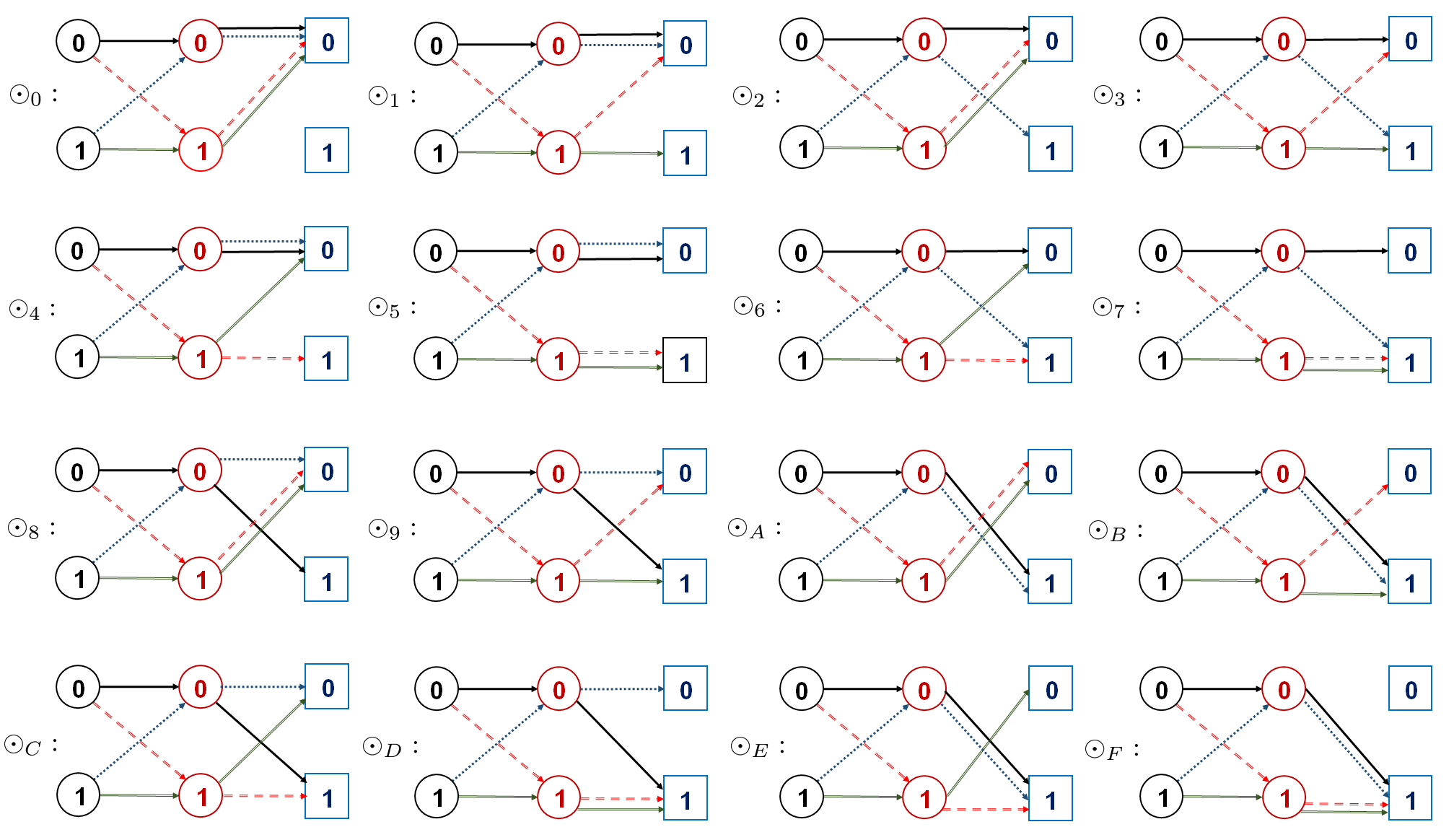
Time is slotted at $t=0,1,\dots$ . Node interactions follow a random gossip process [17], where independently at each time $t\geq 0$ , a pair of nodes $i$ and $j$ with $\{i,j\}\in\mathrm{E}$ is randomly selected over the graph. Each node $i$ holds a binary value from the set $\{0,1\}$ at each time $t$ , denoted $x_{i}(t)$ . Note that, there are a total of $16$ Boolean functions with two arguments mapping from $\{0,1\}^{2}$ to $\{0,1\}$ . Using hexadecimal numbers, we index these functions in the set (see Fig. 1)

\mathsf{H}:=\{\odot_{0},\dots,\odot_{9},\odot_{A},\dots,\odot_{F}\},

where¹¹ 1 These Boolean functions have their respective names, for which we refer to [30]. each $\odot_{k}$ specifies a binary Boolean function in the way that $a\odot_{k}b$ is the value of the function with arguments $(a,b)$ . Let $\mathsf{C}\neq\emptyset$ be a subset of $\mathsf{H}$ specifying potential node interaction rules along the edges. Let $q:=|\mathsf{C}|$ be the cardinality of the set $\mathsf{C}$ . We index the elements in $\mathsf{C}$ by

\odot_{\mathsf{C}_{1}},\dots,\odot_{\mathsf{C}_{q}}.

Suppose the node pair $\{i,j\}$ is selected at time $t$ . Introduce $p_{1},\dots,p_{q}>0$ satisfying $\sum_{k=1}^{q}p_{k}=1$ . Independent with time and pair selections, the evolution of the $x_{m}(t)$ is determined by

\begin{cases}x_{i}(t+1)=x_{i}(t)\odot_{\mathsf{C}_{k}}x_{j}(t),&\text{with prob. $p_{k},k=1,\dots,q$;}\\ x_{j}(t+1)=x_{j}(t)\odot_{\mathsf{C}_{l}}x_{i}(t),&\text{with prob. $p_{l},l=1,\dots,q$;}\\ x_{m}(t+1)=x_{m}(t),&\text{$m\notin\{i,j\}$},\end{cases}

(1)

where the updates of nodes $i$ and $j$ are independent with each other.

1.3 Induced Markov Chain

Let $X_{t}=(x_{1}(t),\dots,x_{n}(t)),t=0,1,\dots$ be the random process driven by the gossip algorithm and the Boolean rules (1). This random process $X_{t},t\geq 0$ defines a $2^{n}$ -state Markov chain $\mathcal{M}_{\mathrm{G}}(\mathsf{C})=(\mathbf{S}_{n},P)$ , where

\mathbf{S}_{n}=\big\{[s_{1}\dots s_{n}]:\ s_{i}\in\{0,1\},i\in\mathrm{V}\big\}

is the state space, and $P$ is the state transition matrix. Then the state transition matrix $P$ is given by

P=\big[P_{[s_{1}\dots s_{n}][q_{1}\dots q_{n}]}\big]\in\mathbb{R}^{2^{n}\times 2^{n}}

with its rows and columns indexed by the elements in $\mathbf{S}_{n}$ , i.e.,

P_{[s_{1}\dots s_{n}][q_{1}\dots q_{n}]}:=\mathbb{P}\Big(X_{t+1}=[q_{1}\dots q_{n}]\Big|X_{t}=[s_{1}\dots s_{n}]\Big).

1.4 Related Work

The proposed randomized Boolean gossip model apparently cover the classical gossip process [17, 18, 19, 20] as a special case. The process (1) is also a special case of the probabilistic Boolean network model [7, 8], where random Boolean interactions are posed pairwise. Therefore conceptually the model (1) under consideration can certainly be placed into the studies of general probabilistic Boolean networks, e.g., [9, 12, 13]. Since the node interaction rules can be an arbitrary set of Boolean functions, this Boolean gossip model is a useful approximation or generalization to existing characterizations to gene regulation [1], social opinion evolution [3], and virus spreading [4].

Gene Regulation. The evolution of gene expressions can be naturally described as a dynamical system where the two quantized levels, ON and OFF, are represented by logic states 1 and 0, respectively. Each gene normally would only interact with a small number of neighbouring genes²² 2 Such number is two or three in Kauffman’s original proposal [1].. Therefore, the proposed Boolean gossip network model at least serves as a good approximation for gene regulator networks, where a pair of genes interact at any given time and the Boolean function rules $\mathsf{C}$ describe random outcomes of the interactions.

Social Voting. Social peers hold binary opinions for certain political or economical issues, where $1$ represents a supportive opinion and $0$ represents a non-supportive one. Peers meet with each other in pairs randomly and exchange their opinions. The two peers independently decide their opinions after the meeting; the Boolean function rules $\mathsf{C}$ describe how they might revise their opinions.

Virus Spreading. Virus spreading across a computer network can be modeled as a Boolean network, where $0$ and $1$ represent infected and healthy computers, respectively [4]. The proposed Boolean gossip process may characterize more possibilities for two computers during an interaction: two computers, infected or not, are both infected ( $\odot_{1}$ ); two computers, infected or not, are both cured ( $\odot_{F}$ ), etc.

The graphical nature of the model (1) makes it possible to go beyond these existing work [9, 12, 13] for more direct and explicit results. Additionally, majority Boolean dynamics [27] and asynchronous broadcast gossiping [28] are related to the model (1) in the way that they describe Boolean interactions between one node and all its neighbors at a given time instant, in contrast to the gossip interaction rule which happens between one node and one of its selected neighbors.

1.5 Contributions and Paper Organization

The proposed random Boolean gossip model is fully determined by the underlying graph $\mathrm{G}$ and the Boolean interaction set $\mathsf{C}$ . Classical (deterministic or probabilistic) Boolean networks also have graphical characterization [7] where a link appears if the state of the end nodes depend on each other in the Boolean updating rules. To the best of our knowledge, few results have been obtained regarding how the structure of the interaction graph influences detailed network state evolution in the study of Boolean networks.

First of all, we study a special network where the Boolean interaction rules in the set $\mathsf{C}$ do not involve the negation, which is termed positive Boolean networks. Using standard theories from Markov chains, we show that the network nodes asymptotically converge to a consensus represented by a binary random variable, whose distribution is studied for large-scale networks in light of mean-field approximation methods. Moreover, by combinatorial analysis the number of communication classes of positive Boolean networks is fully characterized with respect to the structure of the underlying interaction graph $\mathrm{G}$ , where surprisingly local cyclic structures can drastically change the number of communication classes of the entire network.

Next, we move to general Boolean interaction rules and study the relation between emergence of absorbing network Boolean dynamics and the network structure. Necessary and sufficient conditions are provided for the induced Markov process $\mathcal{M}_{\mathrm{G}}(\mathsf{C})$ to be an absorbing chain. Interestingly, for the majority of the Boolean interaction rules, except for nine of the $2^{16}-1$ possible nonempty sets of binary Boolean functions, whether the induced chain is absorbing does not rely on the network topology as long as the underlying graph is connected; for the remaining nine sets of binary Boolean functions, absorbing property of the induced chain is fully determined by whether the underlying graph $\mathrm{G}$ contains an odd cycle.

The remainder of this paper is organized follows. Section 2 investigates positive Boolean dynamics in terms of steady-state distribution and communication classes. Section 3 further studies general Boolean dynamics with a focus on how the interaction graph determines absorbing Markov chains along the random Boolean dynamics. Finally Section 4 concludes the paper with a few remarks.

2 Positive Boolean Gossiping

In this section, we consider a special case where the Boolean interaction rules in the set $\mathsf{C}$ do not involve the negation $\neg$ . Note that conventionally “ $\wedge$ ” represents Boolean “AND” operation, while “ $\vee$ ” represents Boolean “OR” operation. We term such types of Boolean interaction as positive Boolean dynamics, and define

\mathsf{C}_{\rm pst}=\{\vee,\wedge\}

as the set of positive Boolean functions. Let us denote $\odot_{\mathsf{C}_{1}}=\vee$ and $\odot_{\mathsf{C}_{2}}=\wedge$ . Let $p_{*}=p_{1}$ be the probability for operation “ $\vee$ ” in the dynamics (1).

2.1 State Convergence

Recall that a state in a Markov chain is called absorbing if it is impossible to leave this state [26]. A Markov chain is called absorbing if it contains at least one absorbing state and it is possible to go from any state to at least one absorbing state in a finite number of steps. In an absorbing Markov chain, the non-absorbing states are called transient.

It is not hard to find that the Markov chain $\mathcal{M}_{\mathrm{G}}(\mathsf{C}_{\rm pst})$ is an absorbing chain with $[0\dots 0]$ and $[1\dots 1]$ being the two absorbing states. Let $I_{k}$ denote the $k$ -by- $k$ identity matrix for any integer $k$ . The state transition matrix $P$ therefore will have the form

P=\left[\begin{array}[]{c|c}I_{2}&0\\ \hline\cr R&Q\end{array}\right],

where the $I_{2}$ block corresponds to the two absorbing states $[0\dots 0]$ and $[1\dots 1]$ , $R$ is a $(2^{n}-2)\times 2$ matrix describing transition from the $2^{n}-2$ transient states to the two absorbing states, and $Q$ is a $(2^{n}-2)\times(2^{n}-2)$ matrix describing the transition between the transient states.

Note that following the definition of $P$ , the rows of the matrix $(I_{2^{n}-2}-Q)^{-1}R$ are indexed by the entries in $\mathbf{S}_{n}\setminus\{[0\dots 0],[1\dots 1]\}$ , and the columns are indexed by $[0\dots 0]$ and $[1\dots 1]$ . Let $\big[(I_{2^{n}-2}-Q)^{-1}R\big]_{X_{0}[1\dots 1]}$ be the $X_{0}$ - $[1\dots 1]$ entry of the matrix $(I_{2^{n}-2}-Q)^{-1}R$ . We can conclude the following result from standard theories for absorbing Markov chains (see Theorem 11.6, pp. 420, [26]).

Proposition 1

Let $X_{0}=X(0)\in\mathbf{S}_{n}\setminus\{[0\dots 0],[1\dots 1]\}$ . There exists a Bernoulli random variable $x_{\ast}$ such that

\mathbb{P}\big(\lim_{t\rightarrow\infty}x_{i}(t)=x_{\ast},\mbox{for all}\ i\in\mathrm{V}\big)=1.

The limit $x_{\ast}$ satisfies

\mathbb{E}\{x_{\ast}\}=\big[(I_{2^{n}-2}-Q)^{-1}R\big]_{X_{0}[1\dots 1]}.

2.2 Communication Classes

We continue to investigate the communication classes of $\mathcal{M}_{\mathrm{G}}(\mathsf{C}_{\rm pst})$ . Recall that a state $[s_{1}\dots s_{n}]$ is said to be accessible from state $[q_{1}\dots q_{n}]$ if there is a nonnegative integer $t$ such that $\mathbb{P}\big(X_{t}=[s_{1}\dots s_{n}]\ \big|\ X_{0}=[q_{1}\dots q_{n}]\big)>0$ . It is termed that $[s_{1}\dots s_{n}]$ communicates with state $[q_{1}\dots q_{n}]$ if $[s_{1}\dots s_{n}]$ and $[q_{1}\dots q_{n}]$ are accessible from each other [26]. This communication relationship forms an equivalence relation among the states in $\mathbf{S}_{n}$ . The equivalence classes of this relation are called communication classes of the chain $\mathcal{M}_{\mathrm{G}}(\mathsf{C}_{\rm pst})$ . The number of communication classes of $\mathcal{M}_{\mathrm{G}}(\mathsf{C}_{\rm pst})$ is denoted as $\chi_{{}_{\mathsf{C}_{\rm pst}}}(\mathrm{G})$ . The following theorem provides a full characterization to $\chi_{{}_{\mathsf{C}_{\rm pst}}}(\mathrm{G})$ .

Theorem 1

There hold

(i)

$\chi_{{}_{\mathsf{C}_{\rm pst}}}(\mathrm{G})=2n$ , if $\mathrm{G}$ is a line graph;
(ii)

$\chi_{{}_{\mathsf{C}_{\rm pst}}}(\mathrm{G})=m+3$ , if $\mathrm{G}$ is a cycle graph with $n=2m$ ; $\chi_{{}_{\mathsf{C}_{\rm pst}}}(\mathrm{G})=m+2$ , if $\mathrm{G}$ is a cycle graph with $n=2m+1$ ;
(iii)

$\chi_{{}_{\mathsf{C}_{\rm pst}}}(\mathrm{G})=5$ , if $\mathrm{G}$ is neither a line nor a cycle, and contains no odd cycle;
(iv)

$\chi_{{}_{\mathsf{C}_{\rm pst}}}(\mathrm{G})=3$ , if $\mathrm{G}$ is not a cycle graph but contains an odd cycle.

Established by constructive proofs that can overcome the fundamental computational obstacle in analyzing large-scale Boolean networks, Theorem 1 reveals how local structures can drastically change the number of communication classes as a global property of networks. The detailed proof of Theorem 1 has been put in the Appendix. Below we present a few examples illustrating the statements of Theorem 1.

Example 1. Let the underlying graph $\mathrm{G}$ be the four-node cycle graph as displayed in Figure 2. With the positive Boolean rules $\mathsf{C}_{\rm pst}$ , the state transition map of the induced Markov chain is illustrated in Figure 3. Clearly the chain has $5$ communication classes, consistent with Theorem 1.

Example 2. Let the underlying graph $\mathrm{G}$ be the four-node graph containing a three-node cycle subgraph as displayed in Figure 4. With the positive Boolean rules $\mathsf{C}_{\rm pst}$ , the state transition map of the induced Markov chain is illustrated in Figure 5. In this case the chain has $3$ communication classes, again verifying Theorem 1.

2.3 Continuous-Time Approximation

It has been clear from Proposition 1 that starting from $X_{0}\in\mathbf{S}_{n}\setminus\{[0\dots 0],[1\dots 1]\}$ , the limit of the node states is fully characterized by $\big[(I_{2^{n}-2}-Q)^{-1}R\big]_{X_{0}[1\dots 1]}$ . However, computing the exact value or even obtaining an approximation for the matrix $(I_{2^{n}-2}-Q)^{-1}R$ is difficult for large networks due to the exponentially increasing dimension of the matrix. In this subsection, using mean-field method [25, 4], we construct a continuous-time differential equation to approximate the behavior of $X(t)$ for large scale networks (see [29] for a detailed survey on differential equation approximations for Markov chains). To this end, we assume that the $x_{i}(0)$ are i.i.d Bernoulli random variables.

2.3.1 Complete Graph

Define

\delta(t)=\sum_{i=1}^{n}x_{i}(t)/n

as the proportion of nodes that take value 1 at time $t$ . Assume the underlying network forms a complete graph. Let the edges be selected uniformly at random at each time step. Denote $\bm{\delta}(t)$ as the expected value of $\delta(t)$ , i.e., $\bm{\delta}(t)=\mathbb{E}\{\delta(t)\}$ .

The density $\delta(t)$ evolves by the following rules:

•

Let the two nodes in the selected pair $\{i,j\}$ hold different values. When $n$ is large, and the graph is complete, this happens with an approximate probability $2\delta(t)(1-\delta(t))$ . The value $\delta(t)$ will increase by ${1}/{n}$ if the two selected nodes both use “ $\vee$ ” operations to update their values, an event with probability ${p_{*}}^{2}$ . The value $\delta(t)$ will decrease by ${1}/{n}$ if the two selected nodes both apply “ $\wedge$ ” operations, an event with probability ${(1-p_{*})}^{2}$ .
•

For all other cases, $\delta(t)$ is unchanged.

As a result, we conclude that

		$\displaystyle\mathbb{E}\{\delta(t+1)-\delta(t)\|\delta(t)\}\approx\frac{1}{n}{p_{*}}^{2}\cdot 2\delta(t)(1-\delta(t))$
		$\displaystyle\ \ -\frac{1}{n}{(1-p_{*})}^{2}\cdot 2\delta(t)(1-\delta(t)).$		(2)

For a complete graph with $n$ nodes, $\mathbb{V}\{\delta(t)\}=\mathbb{E}\{\delta^{2}(t)\}-\mathbb{E}^{2}\{\delta(t)\}$ can be considered very small for large $n$ . We further have

		$\displaystyle\bm{\delta}(t+1)-\bm{\delta}(t)$
		$\displaystyle\approx\frac{1}{n}{p_{}}^{2}\cdot 2\bm{\delta}(t)(1-\bm{\delta}(t))-\frac{1}{n}{(1-p_{})}^{2}\cdot 2\bm{\delta}(t)(1-\bm{\delta}(t)).$		(3)

Define $s={t}/{n}$ and $\tilde{\bm{\delta}}(s)=\bm{\delta}(ns)=\bm{\delta}(t)$ . Then, (3) can be written as

		$\displaystyle\tilde{\bm{\delta}}(s+{1}/{n})-\tilde{\bm{\delta}}(s)$
		$\displaystyle\approx\frac{1}{n}{p_{}}^{2}\cdot 2\tilde{\bm{\delta}}(s)(1-\tilde{\bm{\delta}}(s))-\frac{1}{n}{(1-p_{})}^{2}\cdot 2\tilde{\bm{\delta}}(s)(1-\tilde{\bm{\delta}}(s))$		(4)

We can therefore approximate (4) for large $n$ by the following differential equation

\frac{d}{ds}\tilde{\bm{\delta}}(s)={p_{*}}^{2}\cdot 2\tilde{\bm{\delta}}(s)(1-\tilde{\bm{\delta}}(s))-{(1-p_{*})}^{2}\cdot 2\tilde{\bm{\delta}}(s)(1-\tilde{\bm{\delta}}(s)),

(5)

whose solution reads analytically as

\tilde{\bm{\delta}}(s)=\frac{\tilde{\bm{\delta}}(0)}{(1-\tilde{\bm{\delta}}(0))e^{2(1-2p_{*})s}+\tilde{\bm{\delta}}(0)}.

(6)

Here $\tilde{\bm{\delta}}(0)=\bm{\delta}(0)=\bm{\delta}_{0}$ is the mean of the i.i.d Bernoulli random variables $x_{i}(0)$ . Consequently, we establish the following approximate equation for $\bm{\delta}(t)$ :

\bm{\delta}(t)=\frac{\bm{\delta}_{0}}{(1-\bm{\delta}_{0})e^{2(1-2p_{*})t/n}+\bm{\delta}_{0}}.

(7)

From (7), the following holds.

Conclusion. Assume $\mathrm{G}$ is a complete graph. For large $n$ , $\bm{\delta}(t)$ approaches zero when $p_{*}<{1}/{2}$ , and $\bm{\delta}(t)$ approaches one when $p_{*}>{1}/{2}$ , as time tends to infinity.

To verify this conclusion, we give some numerical results.

Example 3. Consider a complete graph with $n=1000$ nodes. Fix $\bm{\delta}_{0}=0.5$ , and we randomly distribute the values of nodes according to $\bm{\delta}_{0}=0.5$ . For $p=0.49$ and $0.51$ , we let the nodes update their values randomly according to (1), respectively. Each experiment is carried out over $T=160000$ time steps, repeated for $2000$ rounds. The average of the resulting $2000$ sample paths approximately give the density of nodes with value one for every $t$ . We compare the numerical simulation with the approximate solution given by (7). Figure 6 shows that (7) approximates the real process (1) remarkably well.

Figure 6: A complete graph with

1000

nodes is considered. The solid lines are the approximate solution given by (7); the dashed lines are drawn according to the simulated realization of the algorithm (1). The continuous-time approximations match the numerical realizations rather precisely.

2.3.2 Regular Graph

A regular graph is a graph where nodes have equal degrees. Suppose node $i$ is selected to initialize a gossip interaction at time $t$ . Because $i$ is uniformly selected from $\mathrm{V}$ , the probability that the selected node $i$ is at state $1$ is $\delta(t)$ . If $\mathrm{G}$ is a regular graph with a random nature³³ 3 This is to say, the distribution of the links should appear somehow independently being close to the concentration of random regular graphs. The approximation can be quite inaccurate for graphs like lattices. and high node degrees where $|N_{i}|=\mathcal{O}(n)$ , the distribution of the random variable

\frac{\sum_{j\in\mathrm{N}_{i}}x_{j}(t)}{|\mathrm{N}_{i}|}

will tend to have a similar distribution with

\frac{\sum_{j\neq i}x_{j}(t)}{n-1},

which is approximately a Bernoulli random variable with mean $\delta(t)$ . Therefore, $\delta(t)$ evolves following similar rule as complete graphs, and the differential equation (7) will continue to be a good approximation for high-degree regular graphs.

Example 4. Consider a regular graph of degree $500$ with $n=1000$ nodes. We select $p=0.49$ and $\bm{\delta}_{0}=0.5$ . Again each experiment is carried out over $T=160000$ time steps, repeated for $2000$ rounds. The average of the resulting $2000$ sample paths allows us to obtain the approximate density of nodes with value $1$ for all $t$ . Figure 7 shows that (7) continues to provide an acceptable approximation of the real process (1).

Figure 7: A regular graph with

1000

nodes is considered where node degree is

500

and

p_{*}=0.49

. The solid line is the approximate solution given by (7) and the dashed line is drawn according to numerical simulation. We see that (7) continues to be a good approximation of (1).

3 General Boolean Dynamics

In this section, we discuss the evolution of (1) under general Boolean interaction set $\mathsf{C}\in 2^{\mathsf{H}}$ , where $2^{\mathsf{H}}$ denotes the set containing all subsets of $\mathsf{H}$ . We are interested in how the induced chain $\mathcal{M}_{\mathrm{G}}(\mathsf{C})$ relies on the underlying graph $\mathrm{G}$ and the set of Boolean interaction rules $\mathsf{C}$ . Particularly, we would like to see when $\mathcal{M}_{\mathrm{G}}(\mathsf{C})$ defines an absorbing chain.

Recall that absorbing states are the states that can never be left once visited. Therefore, absorbing Markov chains behave fundamentally different with non-absorbing chains. We introduce two subsets of Boolean mappings:

\mathfrak{B}_{1}=\big\{\mathsf{C}\neq\{\odot_{A}\}\in 2^{\mathsf{H}}:\ \{\odot_{A}\}\subset\mathsf{C}\subseteq\{\odot_{2},\odot_{3},\odot_{A},\odot_{B}\}\big\}

and

\mathfrak{B}_{2}=\big\{\mathsf{C}\in 2^{\mathsf{H}}:\ \{\odot_{2},\odot_{B}\}\subseteq\mathsf{C}\subseteq\{\odot_{2},\odot_{3},\odot_{A},\odot_{B}\}\big\}.

We further let $\mathfrak{B}:=\mathfrak{B}_{1}\mathbin{\mathchoice{\vbox{\hbox{$\textstyle\bigcup$}}}{\vbox{\hbox{$\textstyle\bigcup$}}}{\vbox{\hbox{$\scriptstyle\bigcup$}}}{\vbox{\hbox{$\scriptscriptstyle\bigcup$}}}}\mathfrak{B}_{2}$ .

Note that there are a total of nine elements in $\mathfrak{B}$ . As we show below, Boolean interaction rules in the set $\mathfrak{B}$ lead to drastically different influences to the absorbing property of the induced chain, compared to the rules outside the set $\mathfrak{B}$ .

3.1 Main Results

We first establish a theorem revealing the connection between the induced Markov chains of any two different underlying graphs when connectivity is assumed.

Theorem 2

Suppose $\mathsf{C}\in 2^{\mathsf{H}}\setminus\mathfrak{B}$ . Then, for any two connected graphs $\mathrm{G}_{1}$ and $\mathrm{G}_{2}$ over the node set $\mathrm{V}$ , $\mathcal{M}_{\mathrm{G}_{1}}(\mathsf{C})$ is an absorbing Markov chain if and only if $\mathcal{M}_{\mathrm{G}_{2}}(\mathsf{C})$ is an absorbing Markov chain.

In view of Theorem 2 and the fact that $\mathrm{G}$ is a connected graph by our standing assumption, whether $\mathcal{M}_{\mathrm{G}}(\mathsf{C})$ being an absorbing chain is fully determined by the interaction rule set $\mathsf{C}$ when $\mathsf{C}$ does not belong to $\mathfrak{B}$ . Next, we present the following theorem establishing a necessary and sufficient condition for the induced chain to be absorbing when the Boolean interaction rules come outside the set $\mathfrak{B}$ .

Theorem 3

Suppose $\mathsf{C}\in 2^{\mathsf{H}}\setminus\mathfrak{B}$ . Then $\mathcal{M}_{\mathrm{G}}(\mathsf{C})$ is an absorbing Markov chain if and only if one of the following two conditions holds

(i)

$\mathsf{C}\subseteq\{\odot_{0},\odot_{1},\odot_{2},\odot_{3},\odot_{4},\odot_{5},\odot_{6},\odot_{7}\}$ ;
(ii)

$\mathsf{C}\subseteq\{\odot_{1},\odot_{3},\odot_{5},\odot_{7},\odot_{9},\odot_{B},\odot_{D},\odot_{F}\}$ .

When the interaction rules $\mathsf{C}$ indeed comes from the set $\mathfrak{B}$ , the following theorem further gives a tight condition on the absorbing property of the induced chain. Specifically, if $\mathsf{C}$ is one of the nine function sets in $\mathfrak{B}$ , the topology of $\mathrm{G}$ fully determines whether the induced chain is absorbing.

Theorem 4

Suppose $\mathsf{C}\in\mathfrak{B}$ . Then $\mathcal{M}_{\mathrm{G}}(\mathsf{C})$ is an absorbing Markov chain if and only if $\mathrm{G}$ does not contain an odd cycle.

Note that, Theorem 2 can actually be inferred from Theorem 3. Theorem 3 and Theorem 4 together present a comprehensive understanding of the absorbing property of the network Boolean evolution. Below we present two examples illustrating the usefulness of Theorems 3 and 4.

Example 5. Consider again the graph $\mathrm{G}$ in Figure 4. With the set of Boolean interaction rules being $\mathsf{C}=\{\odot_{2},\odot_{3}\}$ , the transition map of the induced Markov chain is illustrated in Figure 8. The chain is absorbing with seven absorbing states: $[0000]$ , $[1010]$ , $[1001]$ $[1000]$ , $[0100]$ , $[0010]$ , and $[0001]$ . This example is consistent with Theorem 3.(i).

Example 6. Let the underlying graph $\mathrm{G}$ be given in Figure 2. Let the set of Boolean interaction rules be $\mathsf{C}=\{\odot_{2},\odot_{B}\}$ . The chain is absorbing as shown in Figure 9 with two absorbing states $[1001]$ and $[0110]$ . This example is consistent with Theorem 4 as the graph does not contain an odd cyle.

Example 7. Let the underlying graph $\mathrm{G}$ be given in Figure 4, and let the set of Boolean interaction rules continue to be $\mathsf{C}=\{\odot_{2},\odot_{B}\}$ . The chain is not absorbing as shown in Figure 10, further confirming the conclusion drawn in Theorem 4 as the graph contains an odd cyle.

3.2 Key Lemma

To simplify the discussion, we introduce some new notations. For any $S=[s_{1}\dots s_{n}]\in\mathbf{S}_{n}$ , we denote $[S0]$ as $[s_{1}\dots s_{n}0]\in\mathbf{S}_{n+1}$ and $[S1]$ as $[s_{1}\dots s_{n}1]\in\mathbf{S}_{n+1}$ . For any $a\in\{0,1\}$ , denote $\overline{a}=1-a$ . We categorize the states into the following five classes:

$\mathbf{C}_{1}(\mathrm{G})=\{[s_{1}\dots s_{n}]:s_{i}=0,\ 1\leq i\leq n\}$ ,

$\mathbf{C}_{2}(\mathrm{G})=\{[s_{1}\dots s_{n}]:s_{i}=1,\ 1\leq i\leq n\}$ ,

$\mathbf{C}_{3}(\mathrm{G})=\{[s_{1}\dots s_{n}]:s_{i}\neq s_{j}\ \text{for any edge }\{i,j\}\ \text{of }\mathrm{G}\}$ ,

$\mathbf{C}_{4}(\mathrm{G})=\{[s_{1}\dots s_{n}]$ : $\exists i,\ j,\ k$ , s.t. $\{i,j\}$ is an edge of $\mathrm{G}$ and $0=s_{i}=s_{j}\neq s_{k}\}$ , and

$\mathbf{C}_{5}(\mathrm{G})=\{[s_{1}\dots s_{n}]$ : $\exists i,\ j,\ k$ , s.t. $\{i,j\}$ is an edge of $\mathrm{G}$ and $1=s_{i}=s_{j}\neq s_{k}\}$ .

We may simply write $\mathbf{C}_{i}$ instead of $\mathbf{C}_{i}(\mathrm{G})$ whenever this simplification causes no confusion.

In this subsection, we establish a key technical lemma regarding whether a state in the $\mathbf{C}_{i}$ can be an absorbing state in terms of the selection of $\mathsf{C}$ .

Lemma 1

(i) The state in $\mathbf{C}_{1}$ is an absorbing state if and only if $\mathsf{C}\subseteq\{\odot_{0},\odot_{1},\odot_{2},\odot_{3},\odot_{4},\odot_{5},\odot_{6},\odot_{7}\}$ .

(ii) The state in $\mathbf{C}_{2}$ is an absorbing state if and only if $\mathsf{C}\subseteq\{\odot_{1},\odot_{3},\odot_{5},\odot_{7},\odot_{9},\odot_{B},\odot_{D},\odot_{F}\}$ .

(iii) A state in $\mathbf{C}_{3}$ is an absorbing state if and only if $\mathsf{C}\subseteq\{\odot_{2},\odot_{3},\odot_{A},\odot_{B}\}$ .

(iv) A state in $\mathbf{C}_{4}\setminus\mathbf{C}_{5}$ is an absorbing state if and only if $\mathsf{C}\subseteq\{\odot_{2},\odot_{3}\}$ .

(v) A state in $\mathbf{C}_{5}\setminus\mathbf{C}_{4}$ is an absorbing state if and only if $\mathsf{C}\subseteq\{\odot_{3},\odot_{B}\}$ .

(vi) A state in $\mathbf{C}_{5}\mathbin{\mathchoice{\vbox{\hbox{$\textstyle\bigcap$}}}{\vbox{\hbox{$\textstyle\bigcap$}}}{\vbox{\hbox{$\scriptstyle\bigcap$}}}{\vbox{\hbox{$\scriptscriptstyle\bigcap$}}}}\mathbf{C}_{4}$ is an absorbing state if and only if $\mathsf{C}\subseteq\{\odot_{3}\}$ .

Proof. (i) Note that $[0\dots 0]\in\mathbf{C}_{1}$ is a state at which any two nodes associated with a common edge must hold the same value $0$ . According to the algorithm (1), $[0\dots 0]$ is an absorbing state if and only if for any $\odot_{i}\in\mathsf{C}$ there holds $0\odot_{i}0=0.$ Thus, $[0\dots 0]$ is an absorbing state if and only if $\mathsf{C}\subseteq\{\odot_{0},\odot_{1},\odot_{2},\odot_{3},\odot_{4},\odot_{5},\odot_{6},\odot_{7}\}$ .

(ii) The proof is similar to that in (i), whose details are omitted.

(iii) Let $S\in\mathbf{C}_{3}$ , at which two nodes sharing a link must hold different values. According to the structure of the algorithmp (1), $S$ is an absorbing state if and only if for any $\odot_{i}\in\mathsf{C}$ , $0\odot_{i}1=0$ and $1\odot_{i}0=1.$ That is, $S$ is an absorbing state, if and only if $\mathsf{C}\subseteq\{\odot_{2},\odot_{3},\odot_{A},\odot_{B}\}$ .

(iv) It is clear that $S\in\mathbf{C}_{4}\setminus\mathbf{C}_{5}$ is an absorbing state if and only if for any $\odot_{i}\in\mathsf{C}$ , there hold

0\odot_{i}0=0,\ 0\odot_{i}1=0,\text{ and }1\odot_{i}0=1.

In other words, $S$ is an absorbing state if and only if $\mathsf{C}\subseteq\{\odot_{2},\odot_{3}\}$ .

The proofs of the statements (v) and (vi) are similar to that of (iv), which are, again omitted. $\square$

3.3 Proof of Theorem 3

This subsection focuses on the proof of Theorem 3.

(Necessity.) Assume $\mathcal{M}_{\mathrm{G}}(\mathsf{C})$ is an absorbing Markov chain.

If both $[0\dots 0]\in\mathbf{C}_{1}$ and $[1\dots 1]\in\mathbf{C}_{2}$ are not absorbing, any state in $\mathbf{C}_{4}$ or $\mathbf{C}_{5}$ cannot be absorbing as well according to Lemma 1(i)-(ii)(iv)-(vi). This leaves the only possibility be that at least one of the states in $\mathbf{C}_{3}$ is absorbing. Thus, $\mathsf{C}\subseteq\{\odot_{2},\odot_{3},\odot_{A},\odot_{B}\}$ from Lemma 1(iii).

Next, we conclude that $\mathsf{C}$ can only be $\{\odot_{A}\}$ by Lemma 1(i)-(ii) since $\mathsf{C}\in 2^{\mathsf{H}}\setminus\mathfrak{B}$ . However, when $\mathsf{C}=\{\odot_{A}\}$ , any state in $\mathbf{C}_{3}$ cannot be accessed by any other states. This contradicts the assumption that $\mathcal{M}_{\mathrm{G}}(\mathsf{C})$ is an absorbing chain. Therefore, we can only conclude that either $[0\dots 0]\in\mathbf{C}_{1}$ or $[1\dots 1]\in\mathbf{C}_{2}$ is absorbing.

If the state $[0\dots 0]$ is absorbing, we obtain

\mathsf{C}\subseteq\{\odot_{0},\odot_{1},\odot_{2},\odot_{3},\odot_{4},\odot_{5},\odot_{6},\odot_{7}\}

according to Lemma 1(i). While if $[1\dots 1]$ is absorbing, we have

\mathsf{C}\subseteq\{\odot_{1},\odot_{3},\odot_{5},\odot_{7},\odot_{9},\odot_{B},\odot_{D},\odot_{F}\}

from Lemma 1(ii). This proves the necessity statement.

(Sufficiency.) We investigate a few cases.

•
Let $\mathsf{C}\subseteq\{\odot_{0},\odot_{1},\odot_{2},\odot_{3},\odot_{4},\odot_{5},\odot_{6},\odot_{7}\}$ . Then $[0\dots 0]$ is absorbing by Lemma 1(i). We divide the case into a few subcases:
1. 1.
  
  If $\mathsf{C}\mathbin{\mathchoice{\vbox{\hbox{$\textstyle\bigcap$}}}{\vbox{\hbox{$\textstyle\bigcap$}}}{\vbox{\hbox{$\scriptstyle\bigcap$}}}{\vbox{\hbox{$\scriptscriptstyle\bigcap$}}}}\{\odot_{0},\odot_{1},\odot_{4},\odot_{5}\}\neq\emptyset$ , there is a positive probability that $\odot_{i}\in\{\odot_{0},\odot_{1},\odot_{4},\odot_{5}\}$ is chosen. Because $1\odot_{i}0=0,$ any state other than $[1\dots 1]$ can transit to state $[0\dots 0]$ in some finite steps with a positive probability. No matter whether $[1\dots 1]$ is absorbing or not, $\mathcal{M}_{\mathrm{G}}(\mathsf{C})$ is an absorbing Markov chain.
2. 2.
  
  Let $\mathsf{C}\mathbin{\mathchoice{\vbox{\hbox{$\textstyle\bigcap$}}}{\vbox{\hbox{$\textstyle\bigcap$}}}{\vbox{\hbox{$\scriptstyle\bigcap$}}}{\vbox{\hbox{$\scriptscriptstyle\bigcap$}}}}\{\odot_{6}\}\neq\emptyset$ and consider the update where $\odot_{6}$ is always selected. Then for any state in $\mathbf{C}_{4}$ or $\mathbf{C}_{3}$ , two nodes with values $0$ and $1$ respectively will both hold value $1$ after the interaction, i.e., the network state enters $\mathbf{C}_{5}$ or $\mathbf{C}_{2}$ . Furthermore, for any state in $\mathbf{C}_{5}$ or $\mathbf{C}_{2}$ , two nodes both holding value $1$ will both hold $0$ after the interaction. Thus, for all states in $\mathbf{C}_{2},\dots,\mathbf{C}_{5}$ , the number of nodes holding value $1$ will be strictly decreasing if $\odot_{6}$ is always present, until the state transits to $[0\dots 0]$ . The chain $\mathcal{M}_{\mathrm{G}}(\mathsf{C})$ is an absorbing Markov chain since we already know $[0\dots 0]$ is an absorbing state.
3. 3.
  
  Assume $\mathsf{C}=\{\odot_{2}\}$ or $\mathsf{C}=\{\odot_{2},\odot_{3}\}$ and let $\odot_{2}$ be chosen. Then any state in $\mathbf{C}_{2}$ or $\mathbf{C}_{5}$ will transit to state in $\mathbf{C}_{4}\setminus\mathbf{C}_{5}$ or $\mathbf{C}_{1}$ in some finite steps. Thus, $\mathcal{M}_{\mathrm{G}}(\mathsf{C})$ is an absorbing Markov chain because all states in $\mathbf{C}_{1}$ , $\mathbf{C}_{3}$ , $\mathbf{C}_{4}\setminus\mathbf{C}_{5}$ are absorbing by Lemma 1.
4. 4.
  
  If $\mathsf{C}=\{\odot_{7}\}$ or $\mathsf{C}=\{\odot_{3},\odot_{7}\}$ , we can use similar discussion in 1) to conclude that any state other than $[0\dots 0]$ can transit to state $[1\dots 1]$ in finite steps. The chain $\mathcal{M}_{\mathrm{G}}(\mathsf{C})$ is an absorbing Markov chain.
5. 5.
  
  Let $\mathsf{C}=\{\odot_{2},\odot_{7}\}$ or $\mathsf{C}=\{\odot_{2},\odot_{3},\odot_{7}\}$ . The scenario is similar to 2), where any state can transit to state $[0\dots 0]$ in finite steps.
6. 6.
  
  If $\mathsf{C}=\{\odot_{3}\}$ , all states are absorbing. Of course $\mathcal{M}_{\mathrm{G}}(\mathsf{C})$ is an absorbing Markov chain.
•

Assume $\mathsf{C}\subseteq\{\odot_{1},\odot_{3},\odot_{5},\odot_{7},\odot_{9},\odot_{B},\odot_{D},\odot_{F}\}$ . The proof is similar to the case above, whose details are omitted.

The proof of Theorem 3 is now complete.

3.4 Proof of Theorem 4

In this subsection, we prove Theorem 4.

If $\mathrm{G}$ contains an odd cycle, $\mathbf{C}_{3}$ is empty. By Lemma 1, no state in $\mathbf{C}_{1}\mathbin{\mathchoice{\vbox{\hbox{$\textstyle\bigcup$}}}{\vbox{\hbox{$\textstyle\bigcup$}}}{\vbox{\hbox{$\scriptstyle\bigcup$}}}{\vbox{\hbox{$\scriptscriptstyle\bigcup$}}}}\mathbf{C}_{2}\mathbin{\mathchoice{\vbox{\hbox{$\textstyle\bigcup$}}}{\vbox{\hbox{$\textstyle\bigcup$}}}{\vbox{\hbox{$\scriptstyle\bigcup$}}}{\vbox{\hbox{$\scriptscriptstyle\bigcup$}}}}\mathbf{C}_{4}\mathbin{\mathchoice{\vbox{\hbox{$\textstyle\bigcup$}}}{\vbox{\hbox{$\textstyle\bigcup$}}}{\vbox{\hbox{$\scriptstyle\bigcup$}}}{\vbox{\hbox{$\scriptscriptstyle\bigcup$}}}}\mathbf{C}_{5}$ is absorbing. As $\mathbf{S}_{n}=\mathbf{C}_{1}\mathbin{\mathchoice{\vbox{\hbox{$\textstyle\bigcup$}}}{\vbox{\hbox{$\textstyle\bigcup$}}}{\vbox{\hbox{$\scriptstyle\bigcup$}}}{\vbox{\hbox{$\scriptscriptstyle\bigcup$}}}}\mathbf{C}_{2}\mathbin{\mathchoice{\vbox{\hbox{$\textstyle\bigcup$}}}{\vbox{\hbox{$\textstyle\bigcup$}}}{\vbox{\hbox{$\scriptstyle\bigcup$}}}{\vbox{\hbox{$\scriptscriptstyle\bigcup$}}}}\mathbf{C}_{3}\mathbin{\mathchoice{\vbox{\hbox{$\textstyle\bigcup$}}}{\vbox{\hbox{$\textstyle\bigcup$}}}{\vbox{\hbox{$\scriptstyle\bigcup$}}}{\vbox{\hbox{$\scriptscriptstyle\bigcup$}}}}\mathbf{C}_{4}\mathbin{\mathchoice{\vbox{\hbox{$\textstyle\bigcup$}}}{\vbox{\hbox{$\textstyle\bigcup$}}}{\vbox{\hbox{$\scriptstyle\bigcup$}}}{\vbox{\hbox{$\scriptscriptstyle\bigcup$}}}}\mathbf{C}_{5}$ , no state is absorbing. Thus, $\mathcal{M}_{\mathrm{G}}(\mathsf{C})$ is not absorbing. On the other hand, if $G$ does not contain an odd cycle, there are two elements in $\mathbf{C}_{3}$ , and we proceed to prove by induction on the number $n$ of nodes that $\mathcal{M}_{\mathrm{G}}(\mathsf{C})$ is an absorbing Markov chain.

For $n=2$ , the conclusion holds straightforwardly. Assume that $\mathcal{M}_{\mathrm{G}}(\mathsf{C})$ is absorbing for $n=l$ . There must be a spanning tree, denoted $\mathrm{G}_{\mathrm{T}_{1}}$ , of $\mathrm{G}$ . We further find a subtree $\mathrm{G}_{\mathrm{T}_{2}}$ of $\mathrm{G}_{\mathrm{T}_{1}}$ with $\mathrm{G}_{\mathrm{T}_{2}}$ containing $l$ nodes of $\mathrm{G}_{\mathrm{T}_{1}}$ . Without loss of generality, let $\mathrm{G}_{\mathrm{T}_{2}}$ contain nodes $1,\dots,l$ of $\mathrm{G}$ . By our induction assumption, $\mathcal{M}_{\mathrm{G}_{\mathrm{T}_{2}}}(\mathsf{C})$ is absorbing.

Now any state in $\mathbf{S}_{l+1}$ can be represented as $[Su]$ , where $S\in\mathbf{S}_{l}$ and $u\in\{0,1\}$ . As $\mathcal{M}_{\mathrm{G}_{\mathrm{T}_{2}}}(\mathsf{C})$ is absorbing, there is a positive probability that in finite steps $S$ transits to a state $S^{*}$ in $\mathbf{C}_{3}(\mathrm{G}_{\mathrm{T}_{2}})$ . Because $\mathrm{G}_{\mathrm{T}_{2}}$ is a subgraph of $\mathrm{G}_{\mathrm{T}_{1}}$ , $[Su]$ can transit to $[S^{*}u]$ in finite steps in $\mathcal{M}_{\mathrm{G}_{\mathrm{T}_{1}}}(\mathsf{C})$ . There will be two cases.

•

If $[S^{*}u]\in\mathbf{C}_{3}(\mathrm{G}_{\mathrm{T}_{1}})$ , for $\mathrm{G}$ contains no odd cycle, $[S^{*}u]\in\mathbf{C}_{3}(\mathrm{G})$ . The proof is done.
•

If $[S^{*}u]\notin\mathbf{C}_{3}(\mathrm{G}_{\mathrm{T}_{1}})$ , there must be some node $j$ associated with node $l+1$ over graph $\mathrm{G}_{\mathrm{T}_{1}}$ . Because $\mathsf{C}\in\mathfrak{B}$ , there is a positive probability that $\odot_{A}$ or $\odot_{B}$ is chosen. Note that $0\odot_{A}0=1$ , $0\odot_{B}0=1$ , $1\odot_{A}1=0$ and $1\odot_{2}1=0$ . Thus, by (1), $[S^{*}u]$ transits to $[S^{*}\overline{u}]$ with positive probability in $\mathcal{M}_{\mathrm{G}_{\mathrm{T}_{1}}}(\mathsf{C})$ . Moreover, $[S^{*}\overline{u}]\in\mathbf{C}_{3}(\mathrm{G}_{\mathrm{T}_{1}})$ . For $\mathrm{G}$ contains no odd cycle, $[S^{*}\overline{u}]\in\mathbf{C}_{3}(\mathrm{G})$ leads to the desired result.

The proof of Theorem 4 is completed.

4 Conclusions

We proposed and investigated a Boolean gossip model, which may be useful in describing social opinion evolution as well as serves as a simplified probabilistic Boolean network. With positive node interactions, it was shown that the node states asymptotically converge to a consensus represented by a binary random variable, whose distribution was studied for large-scale complete networks in light of mean-field approximation methods. By combinatorial analysis the number of communication classes of the positive Boolean network was counted against the topology of the underlying interaction graph. With general Boolean interaction rules, the emergence of absorbing network Boolean dynamics was explicitly characterized by the network structure. It turned out that local structures in terms of existence of cycles can drastically change fundamental properties of the Boolean network. In future, it will be interesting to look into the possibility of extending the graphical analysis established in the current work to multi-state Boolean networks [14, 15] where each node may hold a state from a finite set with more than two values.

Appendix. Proof of Theorem 1

For each $n$ , we use ${\rm Mod}_{n}(i)$ to denote the unique integer $j$ satisfying $1\leq j\leq n$ and $i\equiv j\mod(n)$ . Recall that for any $a\in\{0,1\}$ , we denote $\overline{a}=1-a$ .

We prove the statements of Theorem 1 in a few steps starting with a few fundamental graphs.

A.1 Line graph

In this subsection we prove Theorem 1.(i) stating that $\chi_{{}_{\mathsf{C}_{\rm pst}}}(\mathrm{G})=2n$ when $\mathrm{G}$ is a line graph. Without loss of generality we assume the edges of $\mathrm{G}$ are $\{i,i+1\}$ for $i=1,\dots,n-1$ . The proof is outlined as follows. We first introduce the notion of $\mathpzc{L}$ -reduced state for each state in $\mathbf{S}_{n}$ . Then, we prove that any two states communicate with each other if and only if their $\mathpzc{L}$ -reduced states are identical. Finally, we count the number of $\mathpzc{L}$ -reduced states in the state space and therefore obtain the number of communication classes.

Definition 1

( $\mathpzc{L}$ -reduced states) Let $[s_{1}\dots s_{n}]\in\mathbf{S}_{n}$ . There exists a unique partition of $s_{1},\dots,s_{n}$ into

\begin{array}[]{ll}s_{1}=\dots=s_{i_{1}}=r_{1},&i_{1}\geq 1;\\ s_{i_{1}+1}=\dots=s_{i_{2}}=r_{2},&i_{2}>i_{1};\\ \dots&\\ s_{i_{d-2}+1}=\dots=s_{i_{d-1}}=r_{d-1},&i_{d-1}>i_{d-2};\\ s_{i_{d-1}+1}=\dots=s_{n}=r_{d}\end{array}

such that $r_{i}\neq r_{i+1}$ for all $i=1,\dots,d-1$ . Then $[r_{1}\dots r_{d}]:=\mathpzc{L}([s_{1}\dots s_{n}])$ is termed the $\mathpzc{L}$ -reduced states of $[s_{1}\dots s_{n}]$ .

Note that the values of any two consecutive elements in an $\mathpzc{L}$ -reduced state are different. The following two lemmas hold.

Lemma 2

Suppose $\mathrm{G}$ is a line graph. Then $\mathpzc{L}([s_{1}\dots s_{n}])$ is a subsequence of $\mathpzc{L}([q_{1}\dots q_{n}])$ if $[s_{1}\dots s_{n}]$ is accessible from $[q_{1}\dots q_{n}]$ . More precisely, denoting

\mathpzc{L}([s_{1}\dots s_{n}])=[r_{1}\dots r_{d}],\ \mathpzc{L}([q_{1}\dots q_{n}])=[h_{1}\dots h_{d^{\prime}}]

there holds $d\leq d^{\prime}$ , and moreover, there exist $1\leq\tau_{1}<\tau_{2}<\dots<\tau_{d}\leq d^{\prime}$ such that $r_{i}=h_{\tau_{i}}$ for all $i=1,\dots,d$ .

Proof. By the definition of accessibility, there is a nonnegative integer $t$ such that

\mathbb{P}\big(X_{t}=[s_{1}\dots s_{n}]\ \big|\ X_{0}=[q_{1}\dots q_{n}]\big)>0.

First we assume $t=1$ . According to the structure of (1), either $[s_{1}\dots s_{n}]=[q_{1}\dots q_{n}]$ , or there is $u\in\{1,\dots,n\}$ such that $s_{u}\neq q_{u}$ and $s_{i}=q_{i}$ for all $i\neq u$ . The desired conclusion obviously holds if $[s_{1}\dots s_{n}]=[q_{1}\dots q_{n}]$ . For the latter case, there is $q_{v}$ with $v=u+1$ or $v=u-1$ such that $q_{u}\neq q_{v}.$ Consequently, the two states $[s_{1}\dots s_{n}]$ and $[q_{1}\dots q_{n}]$ differ with each other only at $s_{u}$ and $q_{u}$ and satisfy

s_{u}\neq q_{u},\ s_{u}=s_{v},\ q_{u}\neq q_{v}.

Then it is easy to verify that $\mathpzc{L}([s_{1}\dots s_{n}])$ is a subsequence of $\mathpzc{L}([q_{1}\dots q_{n}])$ from the definition of $\mathpzc{L}$ -reduced states.

Now we proceed to let $t=2$ . There will be a state $[w_{1}\dots w_{n}]$ such that $[s_{1}\dots s_{n}]$ is one step accessible from $[w_{1}\dots w_{n}]$ , and $[w_{1}\dots w_{n}]$ is one step accessible from $[q_{1}\dots q_{n}]$ . Utilizing the above understanding for the case with $t=1$ we know $\mathpzc{L}([s_{1}\dots s_{n}])$ is a subsequence of $\mathpzc{L}([w_{1}\dots w_{n}])$ and $\mathpzc{L}([w_{1}\dots w_{n}])$ is a subsequence of $\mathpzc{L}([q_{1}\dots q_{n}])$ , which in turn imply $\mathpzc{L}([s_{1}\dots s_{n}])$ is a subsequence of $\mathpzc{L}([q_{1}\dots q_{n}])$ . Therefore the desired conclusion holds for $t=2$ . Apparently the argument can be recursively carried out and the result holds for arbitrary integer $t$ . We have now completed the proof of the lemma. $\square$

Lemma 3

Let $\mathrm{G}$ be a line graph and consider $S=[s_{1}\dots s_{n}],Q=[q_{1}\dots q_{n}]\in\mathbf{S}_{n}$ . Then $S$ and $Q$ communicate with each other if and only if they have identical $\mathpzc{L}$ -reduced states.

Proof. The necessity part of this lemma follows directly from Lemma 2. In the following we focus only on the sufficiency part. Let the identical $\mathpzc{L}$ -reduced state of $[s_{1}\dots s_{n}]$ and $[q_{1}\dots q_{n}]$ be $[r_{1}\dots r_{l}]$ . We carry out an induction argument on $l$ for any $n\geq l$ .

Let $l=1$ . Then $[0\dots 0]_{n}$ and $[1\dots 1]_{n}$ are the two possible states for $[s_{1}\dots s_{n}]$ and $[q_{1}\dots q_{n}]$ . The desired conclusion holds straightforwardly. Now assume:

Induction Hypothesis: The statement of the lemma holds true for all $l\leq k$ and all $n\geq l$ .

We proceed to prove the statement for $l=k+1$ and $n\geq l$ . Denote $i_{1}=\max\{h:r_{1}=s_{i},\ 1\leq i\leq h\}$ and $j_{1}=\max\{h:r_{1}=q_{i},\ 1\leq i\leq h\}$ . By symmetry we may assume $i_{1}\leq j_{1}$ and we use the following two observations:

a)

The state $[q_{1}\dots q_{n}]$ communicates with the state

$[q_{1}\dots q_{i_{1}}\overline{q}_{i_{1}+1}\dots\overline{q}_{j_{1}}q_{j_{1}+1}\dots q_{n}]$

by the definition of $j_{1}$ .
b)

The two states $[\overline{q}_{i_{1}+1}\dots\overline{q}_{j_{1}}q_{j_{1}+1}\dots q_{n}]$ and $[s_{i_{1}+1}s_{i_{1}+2}\dots s_{n}]$ have the same $\mathpzc{L}$ -reduced state $[r_{2}\dots r_{l}]$ . Therefore by our induction hypothesis, $[\overline{q}_{i_{1}+1}\dots\overline{q}_{j_{1}}q_{j_{1}+1}\dots q_{n}]$ and $[s_{i_{1}+1}\dots s_{n}]$ communicate with each other, which in turn yields that $[s_{1}\dots s_{n}]$ communicates with

$[q_{1}\dots q_{i_{1}}\overline{q}_{i_{1}+1}\dots\overline{q}_{j_{1}}q_{j_{1}+1}\dots q_{n}].$

Combining $a)$ and $b)$ we immediately know that $[s_{1}\dots s_{n}]$ communicates with $[q_{1}\dots q_{n}]$ . By the principle of mathematical induction we have completed the proof of the lemma. $\square$

We are now ready to count the number of communication classes for the line graph, which equals to the number of $\mathpzc{L}$ -reduced states according to Lemma 3. For each $m=1,\dots,n$ , there are two different $\mathpzc{L}$ -reduced states with length $m$ , i.e., $[r_{1}\dots r_{m}]$ with $r_{1}=0$ or $r_{1}=1$ . Consequently, there are a total of $2n$ different $\mathpzc{L}$ -reduced states. This concludes the proof for Theorem 1.(i).

A.2 Cycle graph

In this subsection, we prove the case with $\mathrm{G}$ being a cycle graph. Without loss of generality, let $\mathrm{G}$ be the cycle graph with edges $\big\{i,{\rm Mod}_{n}(i+1)\big\}$ , $i=1,\dots,n$ .

We introduce some useful notations that will be used subsequently. For any $k$ , we use $\sigma_{k}$ to denote the permutation on set $\{1,\dots,k\}$ with $\sigma_{k}(i)={\rm Mod}_{k}(i+1)$ for $i=1,\dots,k$ . We further define $\mathpzc{P}_{\sigma_{k}}$ as a mapping over $\mathbf{S}_{k}$ by

\mathpzc{P}_{\sigma_{k}}([s_{1}\dots s_{k}])=[s_{\sigma_{k}(1)}\dots s_{\sigma_{k}(k)}]

for all $[s_{1}\dots s_{k}]\in\mathbf{S}_{k}$ . Intuitively, if we place these $k$ nodes uniformly on a cycle and denote the value of each node on them, then the result of $\mathpzc{P}_{\sigma_{k}}$ on a state is obtained by rotating all the values counterclockwise. We also define a mapping ${f}_{[k_{1},k_{2}]}$ over $\mathbf{S}_{n}$ by that for any $[t_{1}\dots t_{n}]$ , ${f}_{[k_{1},k_{2}]}\big([t_{1}\dots t_{n}]\big)=[r_{1}\dots r_{n}]$ with $r_{i}=t_{i}$ for $i\neq k_{2}$ and $r_{i}=t_{k_{1}}$ for $i=k_{2}$ .

Definition 2

( $\mathpzc{K}$ -reduced states) Let $[s_{1}\dots s_{n}]\in\mathbf{S}_{n}$ with $[r_{1}\dots r_{d}]=\mathpzc{L}([s_{1}\dots s_{n}])$ being its $\mathpzc{L}$ -reduced states. The $\mathpzc{K}$ -reduced states of $[s_{1}\dots s_{n}]\in\mathbf{S}_{n}$ , denoted $\mathpzc{K}([s_{1}\dots s_{n}])$ , is defined as follows:

\mathpzc{K}([s_{1}\dots s_{n}])=\begin{cases}[r_{1}]&\quad\text{if }d=1;\\ [r_{1}\dots r_{d}]&\quad\text{if $d>1$ and $r_{d}\neq r_{1}$};\\ [r_{1}\dots r_{d-1}]&\quad\text{if $d>1$ and $r_{d}=r_{1}$}.\\ \end{cases}

Let $|\mathpzc{K}(S)|$ be the number of digits in $\mathpzc{K}(S)$ for $S\in\mathbf{S}_{n}$ . According to the definition, the values of any two consecutive elements of $\mathpzc{K}$ -reduced states are different. Moreover, if there are at least two entries of $\mathpzc{K}$ -reduced states, the first entry is different from the last one. The following lemma can be established using a similar analysis as we used in Lemma 2.

Lemma 4

Suppose $\mathrm{G}$ is a cycle graph,

(i) $|\mathpzc{K}(S)|$ is either $1$ or an even integer;

(ii) If $d$ is one or an even integer, then there is $S\in\mathbf{S}_{n}$ with $|\mathpzc{K}(S)|=d$ .

(iii) If $S$ is accessible from $T$ , then $|\mathpzc{K}(S)|\leq|\mathpzc{K}(T)|$ .

Lemma 5

Consider $S,T\in\mathbf{S}_{n}$ . If $1<|\mathpzc{K}(S)|=|\mathpzc{K}(T)|<n$ , then $S$ and $T$ communicate with each other.

Proof. Denote $S=[s_{1}\dots s_{n}]$ and $T=[t_{1}\dots t_{n}]$ . We prove this lemma in a few steps.

Step 1. We first prove that $S$ communicates with $\mathpzc{P}_{\sigma_{n}}^{l}(S)$ for any integer $l$ if $|\mathpzc{K}(S)|<n$ . Note that if $|\mathpzc{K}(S)|=1$ , $S$ must be $[0\dots 0]_{n}$ or $[1\dots 1]_{n}$ . The claim holds straightforwardly.

Now we assume $|\mathpzc{K}(S)|>1$ . Since $|\mathpzc{K}(S)|<n$ , the set

\mathcal{I}:=\{i:s_{i}=s_{{\rm Mod}_{n}(i+1)},\ 1\leq i\leq n\}

is nonempty. Moreover, because $|\mathpzc{K}(S)|>1$ , we can find $j\in\mathcal{I}$ such that $s_{{\rm Mod}_{n}(j+1)}\neq s_{{\rm Mod}_{n}(j+2)}$ . By the structure of (1), the state ${f}_{[{\rm Mod}_{n}(j+2),{\rm Mod}_{n}(j+1)]}(S)$ is accessible from $S$ . By the definition of $j$ , there holds

{f}_{[j,{\rm Mod}_{n}(j+1)]}{f}_{[{\rm Mod}_{n}(j+2),{\rm Mod}_{n}(j+1)]}(S)=S.

That is to say, the state $S$ is accessible from

{f}_{[{\rm Mod}_{n}(j+2),{\rm Mod}_{n}(j+1)]}(S).

Therefore, $S$ communicates with ${f}_{[{\rm Mod}_{n}(j+2),{\rm Mod}_{n}(j+1)]}(S)$ . Applying this argument recursively, we obtain that $S$ communicates with

{f}_{[{\rm Mod}_{n}(j+n),{\rm Mod}_{n}(j+n-1)]}\dots{f}_{[{\rm Mod}_{n}(j+2),{\rm Mod}_{n}(j+1)]}(S),

a state equal to $\mathpzc{P}_{\sigma_{n}}(S)$ . It is then convenient to conclude that $S$ communicates with $\mathpzc{P}_{\sigma_{n}}^{l}(S)$ for any integer $l$ .

Step 2. In this step, we prove that if $S=[s_{1}\dots s_{n}]$ and $T=[t_{1}\dots t_{n}]$ have identical $\mathpzc{K}$ -reduced states, then $S$ and $T$ communicate with each other. Let $\mathpzc{K}(S)=\mathpzc{K}(T)=[c_{1}\dots c_{d}]$ . If $d=1$ or $n$ , it is easy to see $S=T$ . Now assume $1<d<n$ .

Because $d>1$ , the sets $\{i:s_{i}\neq s_{0}\}$ and $\{i:t_{i}\neq t_{0}\}$ are not empty. Denote $j_{1}=\max\{i:\ s_{i}\neq s_{0}\}$ , and $j_{2}=\max\{i:\ t_{i}\neq t_{0}\}$ . Without loss of generality we assume $j_{1}>j_{2}$ . Apparently $T$ communicates with ${f}_{[j_{2},j_{2}+1]}(T)$ . Further we know that $T$ communicates with

T^{*}=[t^{*}_{1}\dots t^{*}_{n}]:={f}_{[j_{1}-1,j_{1}]}\dots{f}_{[j_{2}+1,j_{2}+2]}{f}_{[j_{2},j_{2}+1]}(T).

Moreover, we can conclude that $j_{1}=\max\{i:\ t^{*}_{i}\neq t^{*}_{0}\}$ , and $T^{*}$ and $T$ have the same $\mathpzc{K}$ -reduced state. So $T^{*}$ and $S$ have the same $\mathpzc{K}$ -reduced state. By the definition of $\mathpzc{K}$ -reduced state and the fact that $j_{1}=\max\{i:\ s_{i}\neq s_{0}\}=\max\{i:\ t^{*}_{i}\neq t^{*}_{0}\}$ , we know that the $\mathpzc{L}$ -reduced state of $S$ is equal to the $\mathpzc{L}$ -reduced state of $T^{*}$ . Define a new line graph $\tilde{\mathrm{G}}$ , whose nodes are the nodes of $\mathrm{G}$ with edges being $\{i,i+1\}$ for $i=1,\dots n-1$ . According to Lemma 3, $S$ also communicates with $T^{*}$ in $\mathcal{M}_{\tilde{\mathrm{G}}}(\mathsf{C}_{\rm pst})$ . Therefore, $S$ communicates with $T^{*}$ in $\mathcal{M}_{\mathrm{G}}(\mathsf{C}_{\rm pst})$ , because $\tilde{\mathrm{G}}$ is a subgraph of $\mathrm{G}$ . Thus, $S$ and $T$ communicate with each other.

Step 3. This step will complete the proof.

Let $d=|\mathpzc{K}(S)|$ . If $\mathpzc{K}(S)=\mathpzc{K}(T)$ , we have known that $S$ and $T$ communicate with each other. We only need to consider the case $\mathpzc{K}(S)\neq\mathpzc{K}(T)$ . Because $|\mathpzc{K}(S)|=|\mathpzc{K}(T)|$ , there must hold that $\mathpzc{K}(T)=\mathpzc{P}_{\sigma_{d}}(\mathpzc{K}(S))$ . For $d>1$ , the set $\{i:s_{i}\neq s_{0}\}$ is nonempty. Define $j=\min\{i:s_{i}\neq s_{0}\}$ . According to Step 1, $S$ communicates with $\mathpzc{P}_{\sigma_{n}}^{j-1}(S)$ . By the definition of $\mathpzc{K}$ -reduced states, we know that the $\mathpzc{K}$ -reduced state of $\mathpzc{P}_{\sigma_{n}}^{j-1}(S)$ is $\mathpzc{P}_{\sigma_{d}}(\mathpzc{K}(S))$ , i.e., $\mathpzc{K}(T)$ . Therefore, $\mathpzc{P}_{\sigma_{n}}^{j-1}(S)$ communicates with $T$ , implying that $S$ communicates with $T$ . $\square$

Now, we are ready to count the number of communication classes. According to Lemma 4, the digit number $d$ of the $\mathpzc{K}$ -reduced states of all the states in the same communication class are identical. Moreover, $d$ can be $1$ or even numbers. If $n=2m$ , there are three cases:

(i)

For $d=1$ , there are two communication classes $\{[0\dots 0]\}$ and $\{[1\dots 1]\}$ .
(ii)

For each $d=2,4,\dots,2m-2$ , according to Lemma 4 and Lemma 5, there is a unique communication class whose elements have $\mathpzc{K}$ -reduced with $d$ digits.
(iii)

For $d=2m$ , the two states $S_{0}:=[s_{1}\dots s_{2m}]$ and $T_{0}:=[\bar{s}_{1}\dots\bar{s}_{2m}]$ with $s_{2i-1}=1$ and $s_{2i}=0$ for $i=1,\dots,m$ , are the only states whose $\mathpzc{K}$ -reduced states are of length $2m$ . Moreover, either $S_{0}$ or $T_{0}$ cannot be accessible from any other state. That is to say, they form two communication classes.

As a result, there are a total of $m+3$ communication classes. We have completed the proof for the case $n=2m$ . The case with $n=2m+1$ can be similarly analyzed, whose detailed proof is omitted. This concludes the proof of Theorem 1(ii).

A.3 Star graph

In this subsection, we prove that $\chi_{{}_{\mathsf{C}_{\rm pst}}}(\mathrm{G})=5$ if $\mathrm{G}$ is a star graph with $n(\geq 4)$ nodes. Note that a connected graph is called a star graph if there is a node such that all the edges of the graph contain this node. This particular node is called the center node of the graph.

The following proposition characterizes the communication classes for $\mathcal{M}_{\mathrm{G}}(\mathsf{C}_{\rm pst})$ over a star graph $\mathrm{G}$ .

Proposition 2

Let $\mathrm{G}$ be a star graph with $n(\geq 4)$ nodes. Then $\chi_{{}_{\mathsf{C}_{\rm pst}}}(\mathrm{G})=5$ . Moreover, letting node $1$ be the center node, the five classes are

$\mathbf{F}_{n}^{1}=\{[s_{1}\dots s_{n}]:s_{i}=0,\ 1\leq i\leq n\}$ ,

$\mathbf{F}_{n}^{2}=\{[s_{1}\dots s_{n}]:s_{i}=1,\ 1\leq i\leq n\}$ ,

$\mathbf{F}_{n}^{3}=\{[s_{1}\dots s_{n}]:s_{1}=0,\ s_{i}=1,\ 2\leq i\leq n\}$ ,

$\mathbf{F}_{n}^{4}=\{[s_{1}\dots s_{n}]:s_{1}=1,\ s_{i}=0,\ 2\leq i\leq n\}$ ,

$\mathbf{F}_{n}^{5}=\{[s_{1}\dots s_{n}]:\exists i,\ j,\ 2\leq i,\ j\leq n,\ s_{i}=0,\ s_{j}=1\}$ .

Proof. Denote $S_{n}^{\langle 1\rangle},\dots,S_{n}^{\langle 4\rangle}$ as the singleton state in $\mathbf{F}_{n}^{1},\dots,\mathbf{F}_{n}^{4}$ , respectively. Moreover, any other state cannot be accessible from $S_{n}^{\langle 1\rangle}$ or $S_{n}^{\langle 2\rangle}$ , while $S_{n}^{\langle 3\rangle}$ or $S_{n}^{\langle 4\rangle}$ cannot be accessible from any other state. Thus, they do form communication classes, respectively. We only need to prove all the elements in $\mathbf{F}_{n}^{5}$ communicate with each other. We prove this by induction.

First, let $n=4$ . There are $12$ elements of $\mathbf{F}_{4}^{5}$ , listed as $[0100]$ , $[0010]$ , $[0001]$ , $[0011]$ , $[0101]$ , $[0110]$ , $[1100]$ , $[1010]$ , $[1001]$ , $[1011]$ , $[1101]$ , $[1110]$ . It is easy to verify that they are in the same communication class.

Assume that for $n=k\geq 4$ , all the elements in $\mathbf{F}_{n}^{5}$ communicate with each other. Now we prove the case for $n=k+1$ . Let $\mathrm{G}$ be a star graph with $k+1$ nodes with node $1$ being its center node. Let $\mathrm{G}^{*}$ be the subgraph of $\mathrm{G}$ with nodes $1,\dots,k$ and all edges containing them in $\mathrm{G}$ . In fact, $\mathrm{G}^{*}$ is a star graph with $k$ nodes. By our induction assumption, all elements in $\mathbf{F}_{k}^{5}$ communicate with each other in $\mathcal{M}_{\mathrm{G}}(\mathsf{C}_{\rm pst})$ . Because $\mathrm{G}^{*}$ is a subgraph of $\mathrm{G}$ , all elements in $\mathbf{A}:=\{[S0]\in\mathbf{S}_{k+1}:S\in\mathbf{F}_{k}^{5}\}$ communicate with each other, and all elements in $\mathbf{B}:=\{[S1]\in\mathbf{S}_{k+1}:S\in\mathbf{F}_{k}^{5}\}$ communicate with each other.

Note that

\mathbf{F}_{k+1}^{5}=\mathbf{A}\mathbin{\mathchoice{\vbox{\hbox{$\textstyle\bigcup$}}}{\vbox{\hbox{$\textstyle\bigcup$}}}{\vbox{\hbox{$\scriptstyle\bigcup$}}}{\vbox{\hbox{$\scriptscriptstyle\bigcup$}}}}\mathbf{B}\mathbin{\mathchoice{\vbox{\hbox{$\textstyle\bigcup$}}}{\vbox{\hbox{$\textstyle\bigcup$}}}{\vbox{\hbox{$\scriptstyle\bigcup$}}}{\vbox{\hbox{$\scriptscriptstyle\bigcup$}}}}\{[S_{k}^{\langle 1\rangle}1],[S_{k}^{\langle 2\rangle}0],[S_{k}^{\langle 3\rangle}0],[S_{k}^{\langle 4\rangle}1]\}.

Introduce $U_{k}^{\langle a\rangle}=[010\dots 0]$ , $U_{k}^{\langle b\rangle}=[101\dots 1]$ , $U_{k}^{\langle c\rangle}=[001\dots 1]$ and $U_{k}^{\langle d\rangle}=[110\dots 0]$ . They are elements of $\mathbf{F}_{k}^{5}$ . It is easy to verify that $[U_{k}^{\langle a\rangle}0]\in\mathbf{A}$ is accessible from $[U_{k}^{\langle a\rangle}1]\in\mathbf{B}$ . Moreover, $[U_{k}^{\langle b\rangle}1]\in\mathbf{B}$ is accessible from $[U_{k}^{\langle b\rangle}0]\in\mathbf{A}$ . Therefore, all elements in $\mathbf{A}\mathbin{\mathchoice{\vbox{\hbox{$\textstyle\bigcup$}}}{\vbox{\hbox{$\textstyle\bigcup$}}}{\vbox{\hbox{$\scriptstyle\bigcup$}}}{\vbox{\hbox{$\scriptscriptstyle\bigcup$}}}}\mathbf{B}$ communicate with each other.

It is straightforward to verify that $[S_{k}^{\langle 2\rangle}0]$ communicates with $[S_{k}^{\langle 3\rangle}0]$ . Also, $[U_{k}^{\langle c\rangle}0]\in\mathbf{A}$ is accessible from $[S_{k}^{\langle 3\rangle}0]$ and $[S_{k}^{\langle 2\rangle}0]$ is accessible from $[U_{k}^{\langle b\rangle}0]\in\mathbf{A}$ . Thus, all elements in $\mathbf{A}\mathbin{\mathchoice{\vbox{\hbox{$\textstyle\bigcup$}}}{\vbox{\hbox{$\textstyle\bigcup$}}}{\vbox{\hbox{$\scriptstyle\bigcup$}}}{\vbox{\hbox{$\scriptscriptstyle\bigcup$}}}}\{[S_{k}^{\langle 2\rangle}0],[S_{k}^{\langle 3\rangle}0]\}$ communicate with each other. Moreover, $[S_{k}^{\langle 1\rangle}1]$ communicates with $[S_{k}^{\langle 4\rangle}1]$ , $[U_{k}^{\langle d\rangle}1]\in\mathbf{B}$ is accessible from $[S_{k}^{\langle 4\rangle}1]$ , and $[S_{k}^{\langle 1\rangle}1]$ is accessible from $[U_{k}^{\langle a\rangle}1]\in\mathbf{B}$ . Therefore, all elements in $\mathbf{B}\mathbin{\mathchoice{\vbox{\hbox{$\textstyle\bigcup$}}}{\vbox{\hbox{$\textstyle\bigcup$}}}{\vbox{\hbox{$\scriptstyle\bigcup$}}}{\vbox{\hbox{$\scriptscriptstyle\bigcup$}}}}\{[S_{k}^{\langle 1\rangle}1],[S_{k}^{\langle 4\rangle}1]\}$ communicate with each other. Summarizing all these relations we know all elements in

\mathbf{F}_{k+1}^{5}=\mathbf{A}\mathbin{\mathchoice{\vbox{\hbox{$\textstyle\bigcup$}}}{\vbox{\hbox{$\textstyle\bigcup$}}}{\vbox{\hbox{$\scriptstyle\bigcup$}}}{\vbox{\hbox{$\scriptscriptstyle\bigcup$}}}}\mathbf{B}\mathbin{\mathchoice{\vbox{\hbox{$\textstyle\bigcup$}}}{\vbox{\hbox{$\textstyle\bigcup$}}}{\vbox{\hbox{$\scriptstyle\bigcup$}}}{\vbox{\hbox{$\scriptscriptstyle\bigcup$}}}}\{[S_{k}^{\langle 1\rangle}1],[S_{k}^{\langle 2\rangle}0],[S_{k}^{\langle 3\rangle}0],[S_{k}^{\langle 4\rangle}1]\}

communicate with each other. This completes the proof of this proposition. $\square$

A.4 Tree

The following result presents a characterization of the number of communication classes for tree graph that is not a line.

Proposition 3

Let $\mathrm{G}$ be a tree, having at least one node with degree greater than $2$ , i.e., $\mathrm{G}$ is not a line graph. Then $\chi_{{}_{\mathsf{C}_{\rm pst}}}(\mathrm{G})=5$ . The five communication classes can be described as follows:

$\mathbf{J}_{n}^{1}=\big\{[s_{1}\dots s_{n}]:\ s_{i}=0,\ 1\leq i\leq n\big\}$ ,

$\mathbf{J}_{n}^{2}=\big\{[s_{1}\dots s_{n}]:\ s_{i}=1,\ 1\leq i\leq n\big\}$ ,

$\mathbf{J}_{n}^{3}=\big\{[s_{1}\dots s_{n}]:$ $s_{1}=0,\ s_{i}\neq s_{j}$ for any edge $\{i,j\}$ of $\mathrm{G}\big\}$ ,

$\mathbf{J}_{n}^{4}=\big\{[s_{1}\dots s_{n}]:\ s_{1}=1,\ s_{i}\neq s_{j}$ for any edge $\{i,j\}$ of $\mathrm{G}\big\}$ , and

$\mathbf{J}_{n}^{5}=\big\{[s_{1}\dots s_{n}]:$ $\exists i,\ j,\ k$ , s.t. $\{i,j\}$ is an edge of $\mathrm{G}$ and $s_{i}=s_{j}\neq s_{k}\big\}$ .

Proof. It is straightforward to verify that any of $\mathbf{J}_{n}^{1}$ , $\mathbf{J}_{n}^{2}$ , $\mathbf{J}_{n}^{3}$ , $\mathbf{J}_{n}^{4}$ contains a unique element, and forms a communication class. We now prove $\mathbf{J}_{n}^{5}$ is a communication class using an induction argument.

For $n=4$ , $\mathrm{G}$ is a star graph which is proved in Proposition 2. Now assume that this proposition holds for $n=l\geq 4$ .

For any tree $\mathrm{G}$ with $l+1$ nodes that is not a line graph, there is a subgraph $\mathrm{G}^{*}$ with $l$ nodes which is still a tree. Without loss of generality, we denote the node not in $\mathrm{G}^{*}$ as node $v_{*}=l+1\in\mathrm{V}$ . We use $v_{0}$ to denote the node with the highest degree in $\mathrm{G}$ (If there are more than one such nodes, we just choose one of them arbitrarily). There is a path $(v_{0},\ v_{1},\ \dots,\ v_{h},\ v_{*})$ connecting node $v_{0}$ and node $v_{*}$ in $\mathrm{G}$ , where $h\geq 0$ is an integer.

By the induction assumption, the communication classes of $\mathcal{M}_{\mathrm{G^{*}}}(\mathsf{C})$ are $\mathbf{J}_{l}^{1},\dots,\mathbf{J}_{l}^{5}$ with each $\mathbf{J}_{l}^{k}$ defined by replacing $n$ with $l$ in $\mathbf{J}_{n}^{k}$ . Denote $\mathbf{A}=\{[S0]\in\mathbf{S}_{l+1}:S\in\mathbf{J}_{l}^{5}\}$ and $\mathbf{B}=\{[S1]\in\mathbf{S}_{l+1}:S\in\mathbf{J}_{l}^{5}\}$ . Note that

\mathbf{J}_{l+1}^{5}=\mathbf{A}\mathbin{\mathchoice{\vbox{\hbox{$\textstyle\bigcup$}}}{\vbox{\hbox{$\textstyle\bigcup$}}}{\vbox{\hbox{$\scriptstyle\bigcup$}}}{\vbox{\hbox{$\scriptscriptstyle\bigcup$}}}}\mathbf{B}\mathbin{\mathchoice{\vbox{\hbox{$\textstyle\bigcup$}}}{\vbox{\hbox{$\textstyle\bigcup$}}}{\vbox{\hbox{$\scriptstyle\bigcup$}}}{\vbox{\hbox{$\scriptscriptstyle\bigcup$}}}}\{[S_{l}^{\langle 1\rangle}1],[S_{l}^{\langle 2\rangle}0],[S_{l}^{\langle 3\rangle}0],[S_{l}^{\langle 4\rangle}1]\}.

Because $\mathrm{G}^{*}$ is a subgraph of $\mathrm{G}$ , all elements in $\mathbf{A}$ communicate with each other, and all elements in $\mathbf{B}$ communicate with each other. Note that if $\mathrm{G}^{*}$ is a star graph with the $v_{h}$ being the center node, $\mathrm{G}$ will be a star graph. This falls to the case discussed in Proposition 2. We assume $\mathrm{G}^{*}$ is not a star graph for the remainder of the proof.

Introduce

U_{l}^{\langle a\rangle}=[0\dots 0\underset{\underset{v_{h}}{\uparrow}}{1}0\dots 0],\ \ U_{l}^{\langle b\rangle}=[1\dots 1\underset{\underset{v_{h}}{\uparrow}}{0}1\dots 1].

We have $U_{l}^{\langle a\rangle}$ , $U_{l}^{\langle b\rangle}\in\mathbf{J}_{l}^{5}$ . It is easy to verify that $[U_{l}^{\langle a\rangle}1]\in\mathbf{B}$ is accessible from $[U_{l}^{\langle a\rangle}0]\in\mathbf{A}$ . Moreover, $[U_{l}^{\langle b\rangle}0]\in\mathbf{A}$ is accessible from $[U_{l}^{\langle b\rangle}1]\in\mathbf{B}$ . Therefore, all elements in $\mathbf{A}\mathbin{\mathchoice{\vbox{\hbox{$\textstyle\bigcup$}}}{\vbox{\hbox{$\textstyle\bigcup$}}}{\vbox{\hbox{$\scriptstyle\bigcup$}}}{\vbox{\hbox{$\scriptscriptstyle\bigcup$}}}}\mathbf{B}$ communicate with each other.

We further denote $S_{l}^{\langle 4\rangle}=[\gamma_{1}\dots\gamma_{l}]$ and $S_{l}^{\langle 3\rangle}=[\beta_{1}\dots\beta_{l}]$ , and then $U_{l}^{\langle c\rangle}:=[\gamma_{1}\dots\gamma_{v_{h}-1}\overline{\gamma_{v_{h}}}\gamma_{v_{h}+1}\dots\gamma_{l}]$ ,
$U_{l}^{\langle d\rangle}:=[\beta_{1}\dots\beta_{v_{h}-1}\overline{\beta_{v_{h}}}\beta_{v_{h}+1}\dots\beta_{l}]$ . It is straightforward to verify that $[S_{l}^{\langle 1\rangle}1]$ communicates with $[U_{l}^{\langle a\rangle}1]\in\mathbf{B}$ , $[S_{l}^{\langle 2\rangle}0]$ communicates with $[U_{l}^{\langle b\rangle}0]\in\mathbf{A}$ , $[S_{l}^{\langle 3\rangle}0]$ communicates with $[U_{l}^{\langle d\rangle}0]\in\mathbf{A}$ , and $[S_{l}^{\langle 4\rangle}1]$ communicates with $[U_{l}^{\langle c\rangle}1]\in\mathbf{B}$ . Thus, any two elements in $\mathbf{J}_{l+1}^{5}$ communicate with each other. $\square$

A.5 Completion of the Proof

The statements (i) and (ii) in Theorem 1 have been proved for the cases of line and cycle graphs. We are now in a place to prove (iii) and (iv) based on our results for tree graphs. According to Proposition 3, for tree graphs without being a line graph, there are five communication classes $\mathbf{J}_{n}^{1}$ , $\mathbf{J}_{n}^{2}$ , $\mathbf{J}_{n}^{3}$ , $\mathbf{J}_{n}^{4}$ and $\mathbf{J}_{n}^{5}$ . Since any connected graph contains a spanning tree, the communication classes of $\mathcal{M}_{\mathrm{G}}(\mathsf{C}_{\rm pst})$ for any connected graph $\mathrm{G}$ that is not a line or cycle, can only be unions of the $\mathbf{J}_{n}^{j}$ , $j=1,\dots,5$ .

Proof of Theorem 1(iii): Suppose $\mathrm{G}$ is neither a line graph nor a cycle graph and it contains no odd cycle. There is a spanning tree of $\mathrm{G}$ , denoted $\mathrm{G}_{\mathrm{T}}$ . For $\mathcal{M}_{\mathrm{G}_{\mathrm{T}}}(\mathsf{C}_{\rm pst})$ , $\mathbf{J}_{n}^{1}$ , $\mathbf{J}_{n}^{2}$ , $\mathbf{J}_{n}^{3}$ , $\mathbf{J}_{n}^{4}$ and $\mathbf{J}_{n}^{5}$ are communication classes. $\mathbf{J}_{n}^{1}$ and $\mathbf{J}_{n}^{2}$ are absorbing states in $\mathrm{G}$ . Because there is no odd cycle, $\mathbf{J}_{n}^{3}$ and $\mathbf{J}_{n}^{4}$ are the states that any pair of nodes associated with a common edge $\mathrm{G}$ share different values. That is to say, $\mathbf{J}_{n}^{3}$ and $\mathbf{J}_{n}^{4}$ cannot be accessible from any other states in $\mathcal{M}_{\mathrm{G}}(\mathsf{C}_{\rm pst})$ . Thus, $\mathbf{J}_{n}^{1}$ , $\mathbf{J}_{n}^{2}$ , $\mathbf{J}_{n}^{3}$ , $\mathbf{J}_{n}^{4}$ and $\mathbf{J}_{n}^{5}$ are still communication classes in $\mathcal{M}_{\mathrm{G}}(\mathsf{C}_{\rm pst})$ , i.e. $\chi_{{}_{\mathsf{C}_{\rm pst}}}(\mathrm{G})=5$ .

Proof of Theorem 1(iv): Now suppose $\mathrm{G}$ contains an odd cycle. Again, there is a spanning tree $\mathrm{G}_{\mathrm{T}}$ of $\mathrm{G}$ . $\mathbf{J}_{n}^{1}$ , $\mathbf{J}_{n}^{2}$ , $\mathbf{J}_{n}^{3}$ , $\mathbf{J}_{n}^{4}$ and $\mathbf{J}_{n}^{5}$ are communication classes in $\mathcal{M}_{\mathrm{G}_{\mathrm{T}}}(\mathsf{C})$ . Also, $\mathbf{J}_{n}^{1}$ and $\mathbf{J}_{n}^{2}$ are absorbing states in $\mathcal{M}_{\mathrm{G}}(\mathsf{C}_{\rm pst})$ . For states in $\mathbf{J}_{n}^{3}$ and $\mathbf{J}_{n}^{4}$ , there is an edge $e^{*}$ belonging to the odd cycle such that the pair nodes of this edge take different values. Now, by choosing another spanning tree $\mathrm{G}_{\mathrm{T}}^{*}$ containing the edge $e^{*}$ , we can prove that elements in $\mathbf{J}_{n}^{3}$ , $\mathbf{J}_{n}^{4}$ and $\mathbf{J}_{n}^{5}$ communicate with each other in $\mathcal{M}_{\mathrm{G}}(\mathsf{C}_{\rm pst})$ . In turn, $\chi_{{}_{\mathsf{C}_{\rm pst}}}(\mathrm{G})=3$ .

References

[1] S. A. Kauffman, “Metabolic stability and epigenesis in randomly constructed genetic nets,” Journal of Theoretical Biology, 22: 437-467, 1969.
[2] J. J. Hopfield, “Neural networks and physical systems with emergent collective computational abilities,” Proceedings of the National Academy of Sciences, vol. 79, no. 8, pp. 2554-2558, April 1982.
[3] R. Karp, C. Schindelhauer, S. Shenker, and B. Vöcking, “Randomized rumor spreading,” Proc. Symp. Foundations of Computer Science, 564-574, 2000.
[4] P. van Mieghem, J. Omic, and R. Kooij, “Virus spread in networks,” IEEE/ACM Transactions on Networking, vol. 17, no. 1, pp 1-14, 2009.
[5] D. Cheng and H. Qi, “Controllability and observability of Boolean control networks,” Automatica, 45: 1659-1667, 2009.
[6] L. Tournier and M. Chaves, “Interconnection of asynchronous Boolean networks, asymptotic and transient dynamics,” Automatica, 49(4), pp. 884-893, 2013.
[7] I. Shmulevich, E. R. Dougherty, S. Kim, and W. Zhang, “Probabilistic Boolean networks: a rule-based uncertainty model for gene regulatory networks,” Bioinformatics, 2: 261-274, 2002.
[8] I. Shmulevich, I. Gluhovsky, pR. F. Hashimoto, E. R. Dougherty, and W. Zhang, “Steaty-state analysis of genetic regulatory networks modeled by probabilistic Boolean networks,” Comp Funct Genomics, 4: 601-608, 2003.
[9] M. Brun, E. R. Dougherty, and I. Shmulevich, “Steady-state probabilities for attractors in probabilistic Boolean networks,” Signal Process, 85: 1993-2013, 2005.
[10] D. Cheng and H. Qi, “A linear representation of dynamics of Boolean networks,” IEEE Transactions on Automatic Control, 55: 2251-2258, 2010.
[11] M. Chaves and A. Carta, “Attractor computation using interconnected Boolean networks: testing growth rate models in E. Coli,” Theoretical Computer Science, [Online] Jul 2014.
[12] R. Pal, “Context-sensitive probabilistic Boolean networks: steady-state properties, redpuction, and steady-state approximation,” IEEE Transactions on Signal Processing, 58(2): 879-890, 2010.
[13] R. Pal and S. Bhattacharya, “Characterizing the effect of coarse-scale PBN modeling on dynamics and intervention performance of genetic regulatory networks represented by stochastic master equation models,” IEEE Transactions on Signal Processing, 58(6): 3341-3351, 2010.
[14] F. D. Sahneh, C. Scoglio, and P. Van Mieghem, “Generalized epidemic mean-field model for spreading processes over multilayer complex networks,” IEEE/ACM Transactions on Networking 21(5): 1609-1620, 2013.
[15] W. J. Richoux and G. C. Verghese, “A generalized influence model for networked stochastic automata,” IEEE Transactions on Systems, Man, and Cybernetics-Part A: Systems and Humans, 41(1): 10-23, 2011.
[16] T. Akutsu, S. Kuhara, O. Maruyama, et al. “A system for identifying genetic networks from gene expression patterns produced by gene disruptions and overexpressions,” Genome Inf., vol. 9, pp. 151¨C160, 1998.
[17] S. Boyd, A. Ghosh, B. Prabhakar and D. Shah, “Randomized gossip algorithms,” IEEE Trans. Information Theory, vol. 52, no. 6, pp. 2508-2530, 2006.
[18] D. Acemoglu, A. Ozdaglar and A. ParandehGheibi, “Spread of (Mis)information in social networks,” Games and Economic Behavior, vol. 70, no. 2, pp. 194-227, 2010
[19] B. Doerr, M. Fouz, and T. Friedrich, “Why rumors spread so quickly in social networks?” Communications of ACM, 55(6): 2012.
[20] D. Shah, “Gossip algorithms,” Foundations and Trends in Networking, vol. 3, no. 1, pp. 1-125, 2008.
[21] S. A. Kauffman. The Origins of Order: Self-organization and Selection in Evolution. New York: Oxford University Press. 1993.
[22] D. G. Green, T. G. Leishman, and S. Sadedin, “The emergence of social consensus in Boolean networks,” Proceedings of the IEEE Symposium on Artificial Life, pp. 402–208, 2007.
[23] H. Kitano. Foundations of Systems Biology. Cambrige: MIT Press, 2001.
[24] L. Tournier and M. Chaves, “Uncovering operational interactions in genetic networks using asynchronous Boolean dynamics,” Journal of Theoretical Biology, 260(2), 196-209, 2009.
[25] J. O. Kephart and S. R. White, “Directed-graph epidemiological models of computer viruses,” Proc. IEEE Comput. Soc. Symp. Research in Security and Privacy, pp. 343-359, pp., 20-22, May 1991.
[26] C. M. Grinstead and J. L. Snell. Introduction to Probability. Second Revised Edition, American Mathematical Society, 2012.
[27] Y. Kanoria and A. Montanari, “Majority dynamics on trees and the dynamic cavity method,” The Annals of Applied Probability, vol. 21, no. 5, 1694-1748, 2011.
[28] H. Amini, M. Draief, and M. Lelarge, “Flooding in weighted sparse random graphs,” SIAM Journal on Discrete Mathematics, 27(1): 1-26, 2013.
[29] R. W. R. Darling, and J. R. Norris, “Differential equation approximations for Markov chains.” Probability Surveys 5(1) 37-79, 2008.
[30] R. E. Simpson. Introductory Electronics for Scientists and Engineers. 2nd ed. Boston, MA: Allyn and Bacon, 1987.