The Higgs-Boson Decay $H\to gg$ up to $\alpha_{s}^{5}$-Order
under the Minimal Momentum Space Subtraction Scheme

The scale-running behavior of the running coupling is controlled by the renormalization group equation or the $\beta$-function

where the symbol “A” stands for an arbitrary renormalization scheme, $a_{\mathrm{A}}=\alpha_{s,\mathrm{A}}/4\pi$ with $\alpha_{s,\mathrm{A}}$ being the strong running coupling under the $\mathrm{A}$-scheme.

By taking the same integral constant as that of Refs.Bardeen:1978yd; Furmanski:1981cw, the solution of Eq.(2) over the power series of $1/L_{A}$ can be written as,

where $L_{\rm A}=\ln\left({\mu_{r}^{2}}/{\Lambda_{\rm A}^{2}}\right)$ and $\Lambda_{\rm A}$ is the asymptotic scale under an arbitrary $\mathrm{A}$-scheme. The $\{\beta^{\mathrm{A}}_{i}\}$-functions under the $\mathrm{\overline{\rm MS}}$-scheme can be found in Refs.O.V.Tarasov; S.A.Larin; T.van; K.G.Chetyrkin; M.Czakon. Under the Landau gauge, the $\{\beta^{\mathrm{A}}_{i}\}$-functions under the mMOM-scheme up to four-loop level are L.von Smekal

where $n_{f}$ stands for the number of active flavors. Thus the $\alpha_{s}$-running is fixed if we know the asymptotic parameter $\Lambda_{\mathrm{mMOM}}$ well, whose value can be determined by using its relation to $\Lambda_{\overline{\rm MS}}$.

It is noted that both $\beta^{\rm mMOM}_{0}$ and $\beta^{\rm mMOM}_{1}$ are the same as those of $\mathrm{\overline{MS}}$-scheme, then, we can apply the extended renormalization group method suggested by Ref.extendedgroup to evolve the $\mathrm{mMOM}$-running coupling $a_{\mathrm{mMOM}}(\mu_{r,\mathrm{mMOM}})$ at the scale $\mu_{r,\mathrm{mMOM}}$ “adiabatically” into the $\overline{\mathrm{MS}}$-running coupling $a_{\mathrm{\overline{MS}}}(\mu_{r,\overline{\mathrm{MS}}})$ at the scale $\mu_{r,\overline{\mathrm{MS}}}$ not only in scale but also in scheme. Thus a more reasonable and accurate perturbative expansion of $a_{\mathrm{\overline{MS}}}(\mu_{r,\overline{\mathrm{MS}}})$ over $a_{\mathrm{mMOM}}(\mu_{r,\mathrm{mMOM}})$ can be achieved Lu:1992nt. As a special case, when taking the same arguments for the running coupling under different schemes, i.e. $\mu_{r,\overline{\mathrm{MS}}}=\mu_{r,\mathrm{mMOM}}\equiv\mu_{r}$, we get a perturbative series

whose first three coefficients are

On the other hand, the coefficients $r_{i}$ have been directly calculated up to four-loop level O.V.Tarasov; A.I.Davydychev; K.G.Chetyrkin3; L.von Smekal; J.A.Gracey2

As a combination of Eqs.(6, 7, 8) and Eq.(9, 10, 11), we obtain the wanted relations among the asymptotic scales $\Lambda_{\rm mMOM}$ and $\Lambda_{\mathrm{\overline{MS}}}$ up to three-loop level, i.e.

where the symbol $\cdots$ stands for higher-order equations derived through a four-loop and even higher level comparisons. The first equation (13) is derived from a two-loop comparison, which equals to the one given by Refs.L.von Smekal; J.A.Gracey2 that is derived via a different approach. As a byproduct, those relations could be treated inversely as a consistency check of the complex high-order coefficients $D_{i}$ calculated in the literature. For example, the equivalence of Eq.(13) and Eq.(14) can be used as a cross-check of the correctness of $D_{2}$ and $D_{3}$.

Under the usual $\mathrm{\overline{MS}}$-scheme, the pQCD prediction for the total decay width $\Gamma(H\to gg)$ up to $n_{\mathrm{th}}$-loop level can be written as

where $\mu_{r}$ stands for an arbitrary choice of renormalization scale, and $\mathcal{C}^{\mathrm{\overline{MS}}}_{i}$ are $i_{\rm th}$-loop coefficients under the $\mathrm{\overline{MS}}$-scheme, whose values up to four-loop level can be found in Ref.P.A.Baikov. With the help of Eqs.(5, 9, 10, 11, 12), it can be transformed into the mMOM-scheme as

where $G_{F}$ is the Fermi constant. For convenience, we put the mMOM-scheme $c_{i,j}$ coefficients with explicit scale dependence in the Appendix. As a further step, following the PMC $R_{\delta}$-scheme PMC4; PMC5, we can transform the $n_{f}$-series into the following $\{\beta^{\rm mMOM}_{i}\}$-power series,

The mMOM-scheme conformal coefficients $r_{i,0}$ with $i=(1,2,3,4)$ and the non-conformal coefficients $r_{i,j}$ with $1\leq j<i\leq 4$ are also put in the Appendix.

The non-conformal $\{\beta^{\rm mMOM}_{i}\}$-terms determine the optimal behavior of the running coupling via RGE. After applying the PMC, i.e. by absorbing/resumming all $\{\beta^{\rm mMOM}_{i}\}$-terms into the running coupling, the pQCD series (18) can be finally simplified into the following scheme-independent conformal series:

Here $Q_{i}$ stands for the PMC scale at each perturbative order, whose values are determined by RGE and are usually different at different orders. Up to four-loop QCD corrections, the LO PMC scale $Q_{1}$, the NLO PMC scale $Q_{2}$ and the $\mathrm{N^{2}}$LO PMC scale $Q_{3}$ are

At the four-loop level, the N³LO PMC scale $Q_{4}$ is undetermined due to unknown higher-order $\{\beta^{\rm mMOM}_{i}\}$-terms, and we set its value as the latest determined PMC scale $Q_{3}$. After applying the PMC, there are two kinds of residual scale dependence. The PMC scales are in perturbative series such that to eliminate all known non-conformal $\beta$-terms properly via RGE. The first one is from the PMC scales themselves, which are due to “uncalculated” high-order $\beta$-terms. The second one is from the final perturbative term, in which we have no $\beta$-terms to set its PMC scale and we usually take it as the final PMC scale determined at one-order lower. Generally, those two residual scale dependence are highly suppressed, and the conventional renormalization scale uncertainty to the total and individual decay widths at each order can thus be greatly suppressed.

We present the total and individual decay widths of $H\to gg$ at $\alpha_{s}^{5}$-order under conventional scale-setting and the mMOM-scheme in Table 2, in which the results are given by varying $\mu_{r}\in[M_{H}/2,4M_{H}]$. $\Gamma_{\rm Total}=\sum_{i}\Gamma_{i}$ stands for total decay width, where $\Gamma_{i}$ stands for the individual decay width at each order with $i={\rm LO}$, ${\rm NLO}$, ${\rm N^{2}LO}$, and ${\rm N^{3}LO}$, respectively. It is found that under conventional scale-setting, the total decay width $\Gamma_{\rm Total}$ increases with the increment of $\mu_{r}$ for $\mu_{r}\precsim 450$ GeV, and then it slightly decreases with the increment of $\mu_{r}$, which changes down to $355$ keV for $\mu_{r}=1\mathrm{TeV}$. Moreover, for the case of $\mu_{r}=M_{H}$, Table 2 shows that the $K$ factor under the mMOM-scheme follows the trends

In comparison to Eq.(1), it indicates that a more convergent pQCD series than that of $\overline{\rm MS}$-scheme can be achieved by using the mMOM-scheme even before applying the PMC scale-setting. After applying the PMC, the pQCD series shall be further improved as

Under conventional scale-setting, a single renormalization scale is “guessed”, which, at high orders, may give a reasonable prediction for a global observable such as the total decay width or total cross section that is close to the experimental result; however, the corresponding predictions for more detailed observables such as the correlations could be inaccurate or even wrong. As an example: The two-loop prediction for the total cross-section of the top-pair production agrees with the CDF and D0 measurements by simply setting the scale as the top-quark mass; however one then finds a large discrepancy with the top-pair forward-backward asymmetry measured at the Tevatron. In contrast, the PMC prediction predicts both the total cross-section and the forward-backward asymmetry correctly pmc1; pmc3; pmc4; Wang:2015lna, which is also confirmed by the PMC analysis of top-pair production at the LHC pmcLHC.

Table 2 shows that by varying $\mu_{r}\in[M_{H}/2,4M_{H}]$, the total decay width under conventional scale-setting shall be changed by about $\pm 2\%$ from its central value at $\mu_{r}=M_{H}$. This indicates that the scale dependence for the total decay width are small at the present $\alpha_{s}^{5}$-order. By analyzing the pQCD series in detail, it is found that the scale errors are rather large for each perturbative term $\Gamma_{i}$, thus such a small scale error ($\pm 2\%$) for the total decay width is due to cancelations among different orders. For definiteness, we define a ratio to show explicitly how the individual decay width $\Gamma_{i}$ at each order changes with different choices of scale, i.e.,

where $\Gamma_{i}$ stands for the individual decay width at each order and $i={\rm LO}$, ${\rm NLO}$, ${\rm N^{2}LO}$, and ${\rm N^{3}LO}$, respectively. Under conventional scale-setting, we get

for $\mu_{r}=M_{H}/2$; we get

for $\mu_{r}=2M_{H}$. Those large $\kappa_{i}$ values indicate that under conventional scale-setting, one cannot decide what is the exact decay width for each perturbative order.

As a comparison, we present the PMC prediction for the total and individual decay widths under the mMOM-scheme in Table 3, in which the results are given by taking $\mu_{r}=$ $M_{H}/2$, $M_{H}$, $2M_{H}$ and $4M_{H}$, respectively. Table 3 shows by varying $\mu_{r}\in[M_{H}/2,4M_{H}]$, the total decay width under PMC scale-setting shall only be changed by about $\pm 1\%$. Moreover, the renormalization scale errors for the individual decay widths $\Gamma_{i}$ have also been greatly suppressed by PMC scale-setting, e.g. except for the NLO ratio $|\kappa_{\rm NLO}|<4\%$, all other $\kappa_{i}$ are less than $0.2\%$ by varying $\mu_{r}$ within the region of $\in[M_{H}/2,4M_{H}]$. This can be explained by the fact that after applying the PMC, we can fix the $\alpha_{s}$-running behavior, or equivalently the renormalization scale, at each perturbative order via the using of RGE.

More specifically, for the present process at the $\alpha_{s}^{5}$-order, we have three PMC scales $Q_{1,2,3}$, which are determined by Eqs.(20, 21, 22). They are functions of the initial scale $\mu_{r}$. Generally, the initial scale $\mu_{r}$ can be chosen arbitrarily, which only needs to be within the perturbative region to ensure the reliability of a pQCD calculation. The PMC adopts the $\{\beta^{\rm mMOM}_{i}\}$-terms, determined by RGE, and fixes the optimal scales of the process. We present the PMC scales versus the initial scale $\mu_{r}$ in Fig.(1). Those optimal PMC scales are smaller than the conventional choice of scale $(M_{H})$ to a certain degree. Fig.(1) shows that the PMC scales $Q_{1,2,3}$ are highly independent on the choice of $\mu_{r}$, and their values are almost fixed to be

This explains why the individual decay widths at each order and the total decay width are highly independent to the initial choice of scale. Thus the conventional scale ambiguity is cured.

The $\{\beta^{\rm mMOM}_{i}\}$-terms are governed by RGE, which are generally different at different orders, thus the PMC scales $Q_{i}$ at different orders are different from each other PMC2. The PMC scales themselves are in perturbative series PMC4; PMC5, i.e., for $H\to gg$ at order $\alpha_{s}^{5}$, the LO PMC scale $Q_{1}$ is at the accuracy of next-to-next-to-leading logarithmic order (NNLLO); the NLO PMC scale $Q_{2}$ is at the accuracy of NLLO; and the N²LO PMC scale $Q_{3}$ is at the accuracy of LLO. This way, the PMC scales can be improved when more-and-more QCD loop corrections are considered, and the unknown higher-order $\{\beta^{\rm mMOM}_{i}\}$-terms shall lead to residual scale dependence. In principal, as shown by Refs.pmc1; pmc3; pmc4; Wang:2015lna; pmcLHC; app1; app2; Shen:2015cta, due to both the $\alpha_{s}$-power suppression and the exponential-suppression, such residual scale dependence is negligible. For the present case, we observe that there is a somewhat larger residual scale uncertainty in comparison to previous PMC applications, i.e. a sizable $\sim 1\%$ residual scale dependence has been found to total decay width. This indicates that there are large contributions from the unknown $\{\beta^{\rm mMOM}_{i}\}$-terms. More explicitly, by using the formulas (20, 21, 22), we obtain

The PMC scale $Q_{1}$ shows a good pQCD convergence as the usual PMC applications. However, the pQCD convergence of $Q_{2}$ is questionable, the magnitude of its NLO term is at the same order of the LO term, which explains the larger residual scale dependence shown by Fig.(1). It also explains why there is somewhat larger residual scale dependence to $\Gamma_{\rm NLO}$, as shown by Table 3. Thus to further improve our PMC predictions, we need to finish even higher-order corrections, such as a five-loop calculation, so as to achieve an accurate NLO PMC scale $Q_{2}$ and a precise prediction of the NLO decay width $\Gamma_{\rm NLO}$ with less residual scale dependence.

In above subsection, we have shown the properties of total decay width at order $\alpha^{5}_{s}$ under the mMOM-scheme. As a step forward, it is helpful to learn how the total decay width $\Gamma(H\to gg)$ behaves before and after the PMC scale-setting when more-and-more loop terms are included. In present subsection, we make a detailed discussion on the properties of total decay width from one-loop level to four-loop level.

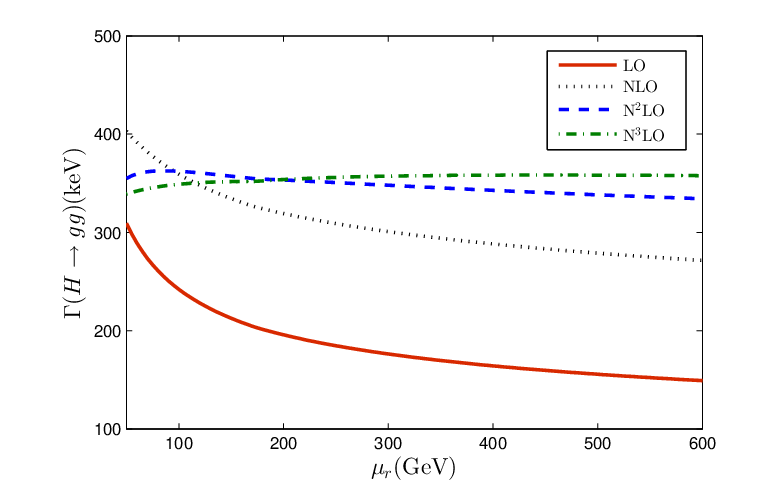
We present the total decay width $\Gamma(H\to gg)$ under the mMOM-scheme versus the initial scale $\mu_{r}$ up to four-loop level before and after the PMC scale-setting in Fig.(2). Fig.(2) shows that under conventional scale-setting, the LO and NLO total decay width $\Gamma(H\to gg)$ depend heavily on $\mu_{r}$, which then becomes weaker-and-weaker when more-and-more loop corrections are taken into consideration; and at the four-loop level, the scale uncertainty of $\Gamma(H\to gg)$ is about $\pm 2\%$ within scale region $\mu_{r}\in[M_{H}/2,4M_{H}]$. This agrees with the conventional wisdom that by finishing a higher-and-higher order calculation, one can get a desirable scale-invariant estimate. However, under conventional scale-setting, by using a single “guessed” scale, the scale ambiguities and scheme-dependence persist at any fixed order: if one uses conventional scale-setting for an $\alpha_{s}^{n}$-order pQCD prediction, the large scale ambiguity exists for any known perturbative terms, as has been shown by the last subsection. On the other hand, it is found that after applying the PMC scale-setting, the total decay width $\Gamma(H\to gg)$ with QCD corrections up to LO, NLO, $\rm N^{2}LO$ and $\rm N^{3}LO$, accordingly, are almost flat versus the scale $\mu_{r}$. Fig.(2) also shows that after the PMC scale-setting, the value of $\Gamma(H\to gg)$ shows a faster steady behavior than the conventional predictions by including higher-and-higher order corrections, e.g. it quickly approaches its steady value with more-and-more loop corrections included.

As shown by Tables 2 and 3, if setting $\mu_{r}=M_{H}/2$ for conventional scale-setting, we get almost the same total decay width as the PMC one. This indicates that for conventional scale-setting, the best choice for $H\to gg$ should be $\sim M_{H}/2$ other than the usually suggested $M_{H}$. Similar choice has been tried for analyzing the gluon-fusion channel $gg\to H$ ggtoh1; ggtoh2; ggtoh3, which has the same topology as the decay $H\to gg$. In Refs.ggtoh1; ggtoh2; ggtoh3, this choice of scale is ‘‘guessed”, and our present derivation provides a reason for this choice ²² 2 A detailed PMC analysis to the important Higgs hadro-production channel, $gg\to H$, is in preparation..

It is helpful to estimate the magnitude of “unknown” higher-order pQCD prediction. We adopt the way suggested by Ref.Wu:2014iba for such an estimation, i.e. for a $n_{\rm th}$-loop pQCD prediction

whose perturbative uncertainty is

which is calculated by varying $\mu_{r}$ within the region of $[M_{H}/2,4M_{H}]$, and the symbol “MAX” stands for the maximum value of $|{\cal C}^{\rm mMOM}_{i}\;a_{\rm mMOM}^{i+1}|$ within this scale region. Under conventional scale-setting, $Q_{i}[\mu_{r}]\equiv\mu_{r}$; under PMC scale-setting, $Q_{i}[\mu_{r}]$ are PMC scales and $\mathcal{C}^{\rm mMOM}_{i}(\mu_{r})\equiv{G_{F}M^{3}_{H}}/{(36\sqrt{2}\pi)}r_{i,0}$ are conformal coefficients. This way of estimating “unknown” higher-order pQCD prediction is natural for PMC, since after the PMC scale-setting, the pQCD convergence is ensured and the only uncertainty is from the last term due to unfixed PMC scale at this particular order.

The fixed-order prediction together with its errors on the total decay width $\Gamma(H\to gg)$ at different pQCD orders before and after the PMC scale-setting are displayed in Fig.(3), in which the “Conv.” stands for the result under conventional scale-setting. In both cases, the predicted error bars from “unknown” higher-order terms show a better agreement with their steady points when more loop-terms are “known”.

To compare with the case of conventional scale-setting, after the PMC scale-setting, the predicted “unknown” higher-order contributions are usually smaller than the conventional ones Wu:2014iba. For the present case, there is one exception that the predicted $\Delta\Gamma^{\rm tot}_{3}$ from a three-loop prediction $\Gamma^{\rm tot}_{3}$ is still large. Numerically it is caused by a smaller NLO PMC scale $Q_{2}$ $(<M_{H})$ and a larger N²LO conformal coefficient $[{G_{F}M^{3}_{H}}/{(36\sqrt{2}\pi)}r_{3,0}]$, which is about two times larger than the N²LO perturbative coefficient $C^{\rm mMOM}_{3}$ ³³ 3 It is noted that a smaller coefficient $C^{\rm mMOM}_{3}$ in comparison to the conformal one is due to the accidentally large cancelation among the conformal and non-conformal terms.. This exception does not indicate the breaking of the general features of the PMC scale-setting, which is consistent with the previous observation that the NLO PMC scale $Q^{2}$ is of large residual uncertainty. In fact, for the present decay channel, the predicted error bars under conventional scale-setting cannot be treated too seriously: the large $\kappa_{i}$ values, as shown by Eqs.(26, 27), indicate that one cannot decide the exact values for all the individual $\Gamma_{i}$ under conventional scale-setting.

References

- (1) G. Aad et al. [ATLAS Collaboration], Phys. Lett. B 716, 1 (2012).
- (2) S. Chatrchyan et al. [CMS Collaboration], Phys. Lett. B 716, 30 (2012).
- (3) T. Inami, T. Kubota and Y. Okada, Z. Phys. C 18, 69 (1983).
- (4) S. Dawson and R. P. Kauffman, Phys. Rev. Lett. 68, 2273 (1992).
- (5) A. Djouadi, M. Spira and P. M. Zerwas, Phys. Lett. B 264, 440 (1991).
- (6) D. Graudenz, M. Spira and P. M. Zerwas, Phys. Rev. Lett. 70, 1372 (1993).
- (7) S. Dawson and R. P. Kauffman, Phys. Rev. D 49, 2298 (1994).
- (8) M. Spira, A. Djouadi, D. Graudenz and P. M. Zerwas, Nucl. Phys. B 453, 17 (1995).
- (9) K. G. Chetyrkin, B. A. Kniehl, and M. Steinhauser, Phys. Rev. Lett. 79, 353 (1997).
- (10) K. G. Chetyrkin, B. A. Kniehl, and M. Steinhauser, Nucl. Phys. B 510, 61 (1998).
- (11) P. A. Baikov and K. G. Chetyrkin, Phys. Rev. Lett. 97, 061803 (2006).
- (12) X. G. Wu, S. J. Brodsky, and M. Mojaza, Prog. Part. Nucl. Phys. 72, 44 (2013).
- (13) S. J. Brodsky and X. G. Wu, Phys. Rev. D 85, 034038 (2012) [Erratum-ibid. D 86, 079903 (2012)].
- (14) S. J. Brodsky and L. Di Giustino, Phys. Rev. D 86, 085026 (2012).
- (15) M. Mojaza, S. J. Brodsky, and X. G. Wu, Phys. Rev. Lett. 110, 192001 (2013).
- (16) S. J. Brodsky, M. Mojaza, and X. G. Wu, Phys. Rev. D 89, 014027 (2014).
- (17) X. G. Wu, Y. Ma, S. Q. Wang, H. B. Fu, H. H. Ma, S. J. Brodsky and M. Mojaza, Rep. Prog. Phys. 78, 126201 (2015).
- (18) S. J. Brodsky and X. G. Wu, Phys. Rev. D 86, 054018 (2012).
- (19) S. J. Brodsky and H. J. Lu, Phys. Rev. D 51, 3652 (1995).
- (20) M. Gell-Mann and F. E. Low, Phys. Rev. 95, 1300 (1954).
- (21) X. G. Wu, S. Q. Wang and S. J. Brodsky, Front. Phys. China 11, 111201 (2016).
- (22) S. Q. Wang, X. G. Wu and S. J. Brodsky, Phys. Rev. D 90, 037503 (2014).
- (23) J. M. Shen, X. G. Wu, H. H. Ma, H. Y. Bi and S. Q. Wang, JHEP 1506, 169 (2015).
- (24) S. Q. Wang, X. G. Wu, X. C. Zheng, J. M. Shen, and Q. L. Zhang, Eur. Phys. J. C 74, 2825 (2014).
- (25) M. Binger and S. J. Brodsky, Phys. Rev. D 74, 054016 (2006).
- (26) W. Celmaster and R. J. Gonsalves, Phys. Rev. Lett. 42, 1435 (1979).
- (27) W. Celmaster and R. J. Gonsalves, Phys. Rev. D 20, 1420 (1979).
- (28) W. Celmaster and R. J. Gonsalves, Phys. Rev. Lett. 44, 560 (1980).
- (29) W. Celmaster and R. J. Gonsalves, Phys. Rev. D 21, 3112 (1980).
- (30) L. von Smekal, K. Maltman, and A. Sternbeck, Phys. Lett. B 681, 336 (2009).
- (31) J. A. Gracey, J. Phys. A: Math. Theor. 46, 225403 (2013).
- (32) S. J. Brodsky, V. S. Fadin, V. T. Kim, L. N. Lipatov, and G. B. Pivovarov, JETP Lett. 70, 155 (1999).
- (33) X. C. Zheng, X. G. Wu, S. Q. Wang, J. M. Shen, and Q. L. Zhang, JHEP 10, 117 (2013).
- (34) M. Hentschinski, A. S. Vera, C. Salas, Phys. Rev. Lett. 110, 041601 (2013).
- (35) F. Caporale, D. Yu. Ivanov, B. Murdaca, and A. Papa, Phys. Rev. D 91, 114009 (2015).
- (36) W. A. Bardeen, A. J. Buras, D. W. Duke and T. Muta, Phys. Rev. D 18, 3998 (1978).
- (37) W. Furmanski and R. Petronzio, Z. Phys. C 11, 293 (1982).
- (38) O. V. Tarasov, A. A. Vladimirov, and A. Yu Zharkov, Phys. Lett. B 93, 429 (1980).
- (39) S. A. Larin and J. A. M. Vermaseren, Phys. Lett. B 303, 334 (1993).
- (40) T. van Bitbergen, J. A. M. Vermaseren, and S. A. Larin, Phys. Lett. B 400, 379 (1997).
- (41) K. G. Chetyrkin, Nucl. Phys. B 710, 499 (2005).
- (42) M. Czakon, Nucl. Phys. B 710, 485 (2005).
- (43) P. M. Stevenson, Phys. Lett. B 100, 61 (1981); Phys. Rev. D 23, 2916 (1981); Nucl. Phys. B 203, 472 (1982); Nucl. Phys. B 231, 65 (1984).
- (44) H. J. Lu and S. J. Brodsky, Phys. Rev. D 48, 3310 (1993).
- (45) O. V. Tarasov, A. A. Vladimirov, and A. Y. Zharkov, Phys. Lett. B 93, 429 (1980).
- (46) A. I. Davydychev, P. Osland, and O. V. Tarasov, Phys. Rev. D 58, 036007 (1998).
- (47) K. G. Chetyrkin and A. Retey, arXiv:hep-ph/0007088.
- (48) ATLAS and CMS Collaborations, ATLAS-CONF-2012-095, CMS-PAS-TOP-12-001.
- (49) K. A. Olive et al. (Particle Data Group), Chin. Phys. C 38, 090001 (2014).
- (50) G.M. Prosperi, M. Raciti, and C. Simolo, Prog. Part. Nucl. Phys. 58, 387 (2007).
- (51) S. J. Brodsky and X. G. Wu, Phys. Rev. Lett. 109, 042002 (2012).
- (52) S. J. Brodsky and X. G. Wu, Phys. Rev. D 85, 114040 (2012).
- (53) S. J. Brodsky and X. G. Wu, Phys. Rev. D 86, 014021 (2012).
- (54) S. Q. Wang, X. G. Wu, Z. G. Si and S. J. Brodsky, Phys. Rev. D 93, 014004 (2016).
- (55) S. Q. Wang, X. G. Wu, Z. G. Si, and S. J. Brodsky, Phys. Rev. D 90, 114034 (2014).
- (56) S. Q. Wang, X. G. Wu, X. C. Zheng, G. Chen, and J. M. Shen, J. Phys. G 41, 075010 (2014).
- (57) S. Q. Wang, X. G. Wu, J. M. Shen, H. Y. Han, and Y. Ma, Phys. Rev. D 89, 116001 (2014).
- (58) C. Anastasiou, K. Melnikov and F. Petriello, Nucl. Phys. B 724, 197 (2005).
- (59) C. Anastasiou, S. Buehler, F. Herzog and A. Lazopoulos, JHEP 12, 058 (2011).
- (60) C. Anastasiou, C. Duhr, F. Dulat, F. Herzog and B. Mistlberger, Phys. Rev. Lett. 114, 212001 (2015).
- (61) G. Aad et al., [The ATLAS and CMS Collaborations], Phys. Rev. Lett. 114, 191803 (2015).