Maps, immersions and permutations

Aix Marseille Université, Université de Toulon, CNRS, CPT, UMR 7332, 13288 Marseille, France
Centre de Physique Théorique (CPT)

and

Sorbonne Universités, UPMC Univ Paris 06, UMR 7589, LPTHE, F-75005, Paris, France
& CNRS, UMR 7589, LPTHE, F-75005, Paris, France

August 24, 2026

We consider the problem of counting and of listing topologically inequivalent “planar” 4-valent maps with a single component and a given number $n$ of vertices. This enables us to count and to tabulate immersions of a circle in a sphere (spherical curves), extending results by Arnold and followers. Different options where the circle and/or the sphere are/is oriented are considered in turn, following Arnold’s classification of the different types of symmetries. We also consider the case of bicolourable and bicoloured maps or immersions, where faces are bicoloured. Our method extends to immersions of a circle in a higher genus Riemann surface. There the bicolourability is no longer automatic and has to be assumed. We thus have two separate countings in non zero genus, that of bicolourable maps and that of general maps.
We use a classical method of encoding maps in terms of permutations, on which the constraints of “one-componentness” and of a given genus may be applied. Depending on the orientation issue and on the bicolourability assumption, permutations for a map with $n$ vertices live in $S_{4n}$ or in $S_{2n}$ .

In a nutshell, our method reduces to the counting (or listing) of orbits of certain subset of $S_{4n}$ (resp. $S_{2n}$ ) under the action of the centralizer of a certain element of $S_{4n}$ (resp. $S_{2n}$ ). This is achieved either by appealing to a formula by Frobenius or by a direct enumeration of these orbits.
Applications to knot theory are briefly mentioned.

Keywords:
Embedded graphs; Knot diagrams; Immersed curves; Closed curves; Topological maps.

Mathematics Subject Classification 2000: 05C10, 05C30, 57M25, 83C47

1 Introduction

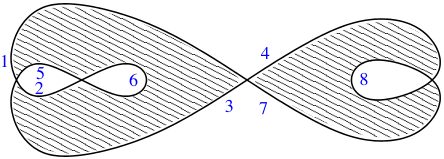
In the present paper we are interested in the problem of enumerating the (equivalence classes of) curves with $n$ double points that one can draw on the sphere or on an orientable surface of genus $g$ . Such curves may be regarded as the images of immersions of a circle in that surface. In the present paper we shall be mainly dealing with immersions in a compact surface. See Fig. 1 for an illustration of the difference between immersions in the plane or in the sphere. The problem is tightly connected with the census of knots and virtual knots but we shall content ourselves with brief comments about knots. Recall that for non zero genus, (virtual) knot diagrams or drawings of curves exhibit virtual crossings in addition to their regular crossings: the former may be regarded as artifacts due to the projection on the plane of the figure, see [1] and the example of Fig. 2.
Since the curves (or the knot diagrams), like the surfaces themselves, can be oriented, the discussion and the results will naturally split into four cases (OO, UO, OU, UU) that we define now: a genus $g$ curve is the image of the circle under an immersion $S^{1}\to\Sigma$ , the latter being an orientable surface of genus $g$ , and, if the curve is not simple (if it crosses itself), the multiple points of the immersion should be double points with distinct tangents (in other words we consider generic closed curves). When $g=0$ , this is called a generic spherical curve. Both the circle and the surface can be oriented. If $S^{1}$ is not oriented, one may consider the sets UU and UO of $\mathrm{Diff}(\Sigma)$ -equivalent and $\mathrm{Diff}^{+}(\Sigma)$ -equivalent unoriented curves. If $S^{1}$ is oriented, one considers the sets OU and OO of $\mathrm{Diff}(\Sigma)$ -equivalent and $\mathrm{Diff}^{+}(\Sigma)$ -equivalent oriented curves. $\mathrm{Diff}^{+}(\Sigma)$ denotes the group of orientation-preserving diffeomorphisms of the oriented surface $\Sigma$ . For spherical curves, these four types of immersions have been considered by previous authors, [2, 3, 4]. Correspondingly, in knot theory one may consider knots up to mirror symmetry, and oriented or unoriented.
Following Carter [5], who coined this adjective in the UU case, one says that two immersed curves are OO, UO, OU or UU geotopic if they are equivalent in the previous sense. Now it is clear that the operation of adding handles to a surface in which a circle is immersed defines immersed curves in higher genus surfaces. It is therefore natural to consider the following definition [5]: two immersed curves are stably geotopic if and only if there is a collection of handles that can be added to either surface, or both, in such a way that the curves become geotopic on the resulting surfaces. In this paper we assume that the studied immersions are cellular, in the sense that the complement of each associated immersed curve is homeomorphic to a collection of open disks, so that the classifications obtained in this paper when $g>0$ for the different kinds of immersions should always be understood up to stable geotopy (although this will not be in general repeated in the text). In other words the genus given in our tables for an immersed curve with a given number of crossings is such that the chosen curve cannot be immersed in a surface of smaller genus. One could then use surgeries to obtain a classification for all generic immersed curves (see [6]).
On top of the question of orientation, we introduce the issue of bicolourability of the curve. By definition a curve is bicolourable if one can assign opposite colors to adjacent faces. While in genus 0, any self intersecting curve may be bicoloured (with adjacent faces of opposite colours), it is no longer true for higher genus, see Fig. 2 for an example. Moreover when a curve is bicoloured, the two possible colourings may be or not (topologically) equivalent, see Fig. 5. This bicolouring is quite natural in the context of knot theory, where it amounts to considering the curve as an alternating knot, see Fig. 9 below; there are two ways of doing that, which may or not lead to equivalent knots. We shall thus append a suffix $c$ , $b$ or no suffix at all to the symbols OO, OU, etc: OOc will refer to (inequivalent) bicolourings of immersions of an oriented circle in an oriented surface, OOb to bicolourable (but not bicoloured) immersions, and OO alone to general, bicolourable or not, immersions. Likewise for immersions of type UO, OU and UU. This results in $3\times 4=12$ different types of immersions, and the reader who is eager to see numbers may jump to Tables 7, 6 to see their cardinals tabulated up to 10 crossings for all genera. The reader who prefers figures to numbers is directed to Fig. 15 and 16-17 for a complete list of indecomposable irreducible spherical curves of UU type, with respectively $n=8$ and 9 crossings.

Figure 1: Immersions of an unoriented circle with two double points. The five immersions in the plane give rise to two distinct immersions on the sphere, for instance the two lying on the left.

Figure 2: The diagram on the left describes a genus 1 immersion and is not bicolourable. The little blue circle encircles a virtual crossing. On the right, the same immersed in a torus.

Figure 3: Two immersions of an unoriented circle with

n=6

double points. Distinct on an oriented sphere, but equivalent on an unoriented sphere.

Figure 4: Immersions of an oriented circle. Left : an

n=3

immersion not equivalent to its reverse; in contrast, the trefoil is equivalent to its reverse.

Refer to caption — Figure 5: Swapping colours : the two diagrams on the top are not equivalent, while the two diagrams on the bottom are (on the sphere, of course). The first two contribute 2 to $|{\rm UUc}|$ and 1 to $|{\rm UUb}|$ , the last two contribute 1 to both.

For $g>0$ immersions they are few explicit results made available in the literature, see however¹¹ 1 The latter reference (that we discovered at a later stage of our work) contains, for the UU case, a table of isomorphism classes of immersions, with given genus and a given number of crossings (up to five), obtained using Gauss diagrams and a method described in [5]. [7] and [8].

We shall regard curves with simple crossings (images of immersions) as 4-valent maps. Our immersions, being cellular, indeed define maps²² 2 They also define cellular embeddings of particular graphs called “simple assembly graphs without endpoints” in [9], see also [10].: recall that a map is a graph embedded in a surface with its 2-cells (aka faces) homeomorphic to open disks. The fact that faces do not contain handles will be used repeatedly in this paper, in particular when using the Euler formula to determine the genus of embedded curves. We should insist on the fact that in this work we consider circle immersions/maps, bicolourable or not: all the curves that we consider have a single connected component (in the language of knot theory, we are interested in knots, not in links).
Matrix integrals in the large size limit which are quite effective for the counting of maps of a given genus fail to distinguish maps with different numbers of components. We thus use an alternative method regarding maps as combinatorial maps, i.e., maps described by pairs of permutations, following an old idea by Walsh and Lehman [12], or some variants. The constraints of “one-componentness” and of fixed genus may be easily enforced in that description. Depending on the orientation issue and on the bicolourability assumption, permutations for a map with $n$ vertices live in $S_{4n}$ or in $S_{2n}$ .
This method, however, yields labelled maps. To obtain unlabelled maps and immersions, a quotient by a relabelling group has to be performed. This is achieved by considering orbits of the combinatorial maps under the action of some subgroup of the permutation group.
The set-up of the paper is as follows. In Sect. 2, we present the simplest version of the previous idea, where the two permutations encoding general immersions live in $S_{4n}$ . The rapid growth of $(4n)!$ limits its practical use beyond $n=6$ . In Sect. 3, we consider bicolourable maps and introduce a better coding by pairs of permutations of $S_{2n}$ . Orbits of these pairs under the action of the hyperoctahedral group yield immersions of type OOc. Sect. 4 is devoted to a study of the various types of bicoloured or bicolourable immersions that may be derived from the OO type. We derive some relations between the numbers of these different types (Theorem 4). In Sect. 5, we remove the assumption of bicolourability and encode the general maps and immersions by another choice for the pair of permutations of $S_{2n}$ . Sect. 6 and 7 gather results, comments on the asymptotia and on the application to knot theory and our conclusions. Appendix A gives some details on the algorithms used for counting orbits, Appendix B contains several tables of interest that will be described later, and Appendix C reviews the connection between maps and Feynman diagrams of matrix or scalar integrals.

A notational comment: in the following, we make use of two notations for the cardinal of a set $X$ , either $|X|$ or $\#X$ .

2 UO immersions, first method using permutations of $S_{4n}$

2.1 The subset $X=[2^{2n}]$ of $S_{4n}$ and its orbits (“X method”)

In the present section, we obtain the number of circle immersions of type UO, with $n$ crossings, by counting the number of orbits of solutions for a particular set of equations written in the group $S_{4n}$ , under the action of a particular subgroup. We shall actually recover part of these results later, with other methods, which are faster (see Sect. 3 and 5), but the technique presented here has an interest of its own.

Method: description of a curve by a permutation belonging to a particular conjugacy class $X$ of $S_{4n}$ .

In a first stage, we consider a labelling of half-edges of the maps. For a 4-valent map with $n$ vertices, there are $4n$ such half-edges, and we consider the symmetric group $S_{4n}$ acting on these labels. We choose $\sigma\in[4^{n}]$ ³³ 3 The notation $[\cdot]$ refers to the conjugacy classes of the permutation group to describe the clockwise linking pattern of half-edges at the vertices, and consider all possible pairings of half-edges (propagators in physicists’ parlance) encoded in permutations $\tau\in[2^{2n}]$ . Note that this method of labelling half-edges is not original, it has been used by Walsh and Lehman [12] and rediscovered later by Drouffe, as quoted in [13].

Example of encoding

See below in Fig. 6 the map encoded by

$\sigma=(1,2,3,4)(5,6,7,8)(9,10,11,12)(13,14,15,16)$

$\tau=(1,13)(2,5)(3,6)(4,16)(7,8)(9,12)(10,15)(11,14)$

in cycle notation.

Orbits of $X=[2^{2n}]$ for the adjoint action of the centralizer of an element of $[4^{n}]$

Theorem 1.

Call $\sigma=(1,2,3,4)(5,6,7,8)\ldots(4n-3,4n-2,4n-1,4n)\in[4^{n}]\subset S_{4n}$ , using cycle notation, and ${\cal C}_{\sigma}=C(S_{4n},\sigma)$ , the centralizer of $\sigma$ in $S_{4n}$ . Let $X=[2^{2n}]$ denote the conjugacy class of $S_{4n}$ whose elements are products of $2n$ transpositions. Then we have :
Circle immersions of type UO, i.e., immersions of the unoriented circle in an orientable and oriented surface of genus $g$ , are in bijection with the orbits of ${\cal C}_{\sigma}$ acting by conjugation on the set of permutations $\tau$ that belong to $X$ and solve the simultaneous equations:

		$\displaystyle\sigma^{2}\tau\in[(2n)^{2}]$	$\displaystyle\qquad\qquad\qquad\,{\rm(I)}\qquad\qquad{\rm one-componentness}$
		$\displaystyle c(\sigma\tau)=n+2-2g$	$\displaystyle\qquad\qquad\qquad{\rm(II)}_{{g}}\qquad\qquad{\rm genus\ condition}$

where $c(x)$ is the function giving the number of cycles (including singletons) of the permutation $x$ .

Proof.

That labelled maps are in one-to-one correspondance with pairs $(\sigma,\tau)$ has been known for long [12]. The sequence of labels as one goes across the crossings is described by the permutation $\sigma^{2}\tau$ , and imposing condition (I) ensures that the curve has a single component (hence also that the graph is connected). Condition (II)_g follows from Euler relation, if one realizes that the number of faces of the map is just the number of cycles $c(\sigma\tau)$ , (another observation made by many previous authors…). A change of labels by $\gamma\in S_{4n}$ acts on $\sigma$ and $\tau$ by conjugation: $(\sigma,\tau)\to(\sigma^{\gamma},\tau^{\gamma})$ , with $\alpha^{\gamma}:=\gamma\alpha\gamma^{-1}$ . The form of $\sigma$ as well as conditions on permutations $\tau$ of the type (I), (II)_g, (I) $\cap$ (II)_g, are invariant under the action of any $\gamma$ in the centralizer ${\cal C}_{\sigma}$ of $\sigma$ , i.e.,

\tau\ {\rm satisfies\ (I)\ and/or\ (II)}_{{g}}\ ,\ \gamma\in{\cal C}_{\sigma}\quad\Longrightarrow\quad\tau^{\gamma}\ {\rm satisfies\ it\ too\,.}

∎

Heuristically, ${\cal C}_{\sigma}$ is the group of reparametrizations (relabellings) of the edges of the diagram that leave the pattern of edges around each vertex unchanged. Quotienting by that group, i.e., considering its orbits for the adjoint action thus enables one to go from labelled maps to unlabelled, topologically distinct maps. Finally note that the definition of $\sigma$ as describing the, say, clockwise linking pattern at vertices has singled out an orientation of the surface, while no information about the orientation of the circuit described by $\sigma^{2}\tau$ is provided: the maps are naturally asssociated with immersions of an unoriented circle in an oriented surface, hence of type UO in our nomenclature.

We shall use the following notations for the relevant subsets of $X=[2^{2n}]$ :

\begin{split}X^{\prime}=&\{\tau\in[2^{2n}]\ |\ \sigma^{2}\,\tau\in[(2n)^{2}]\}\\ X^{\prime}_{g}=&\{\tau\in[2^{2n}]\ |\ \sigma^{2}\,\tau\in[(2n)^{2}]\ \ \text{and}\ \sigma\,\tau\ {\rm has\ }n+2-2g\ {\rm cycles}\}\,.\end{split}

In particular we denote $X^{\prime\prime}=X^{\prime}_{0}$ , corresponding to planar (in fact spherical) maps. The family of sets $X^{\prime}_{g}$ is a partition of $X^{\prime}$ , and the set of orbits of the latter (identified with circle immersions), for the adjoint action of the subgroup ${\cal C}_{\sigma}$ , is also partitioned into orbits corresponding to the various circle immersions of genus $g$ .

Remarks.
(i) In the group $S_{4n}$ , the function $c$ is related to the ( $n$ -independent) length function $\ell$ by $\ell(x)=4n-c(x)$ . Therefore equation (II)_g also reads $\ell(\sigma\tau)=3n-2+2g$ .
(ii) In the wording of the theorem we made a convenient choice for $\sigma$ ; this is actually irrelevant since the choice amounts to labelling the half-edges in a specific way.
(iii) An arbitrary curve has $c(\sigma\tau)=n+2-2g\geq 1$ , therefore the possible values of $g$ are such that $2g\leq n+1$ .

Examples.

Let us choose $n=4$ , then
$\sigma=(1,2,3,4)(5,6,7,8)(9,10,11,12)(13,14,15,16)$ in cycle notation, equivalently
$\sigma=[2,3,4,1,6,7,8,5,10,11,12,9,14,15,16,13]$ in list notation.

First example: $\tau=(1,13)(2,5)(3,6)(4,16)(7,8)(9,12)(10,15)(11,14)$ .
One checks that $\sigma^{2}\tau=(1,15,12,11,16,2,7,6)(3,8,5,4,14,9,10,13)\in[8^{2}]$ , so $\tau$ obeys condition (I) and therefore encodes an immersion (possibly non-spherical). One then evaluates $\sigma\tau=(1,14,12,10,16)(2,6,4,13)(3,7,5)(11,15)$ ; its number of cycles is $6$ (there are two unwritten⁴⁴ 4 Since $n$ is fixed, it is unnecessary to write explicitly the 1-cycles when using the cycle notation, but one should remember that the function $c(x)$ should count the total number of cycles ! singletons: (8) and (9), so that the genus is $0$ , and the immersion is actually spherical. The immersion encoded by permutation $\tau$ is given in Fig. 6. Notice that $1$ -cycles give rise (or come from) kinks, also known as simple loops.

Figure 6: The diagram encoded by

\tau=(1,13)(2,5)(3,6)(4,16)(7,8)(9,12)(10,15)(11,14)

Second example: $\tau=(1,8)(2,3)(4,16)(5,13)(6,12)(7,14)(9,15)(10,11)$ .
One checks that $\sigma^{2}\tau=(1,6,10,9,13,7,16,2)(3,4,14,5,15,11,12,8)\in[8^{2}]$ , but this time $\sigma\tau=(1,5,14,8,2,4,13,6,9,16)(7,15,10,12)$ which has two 1-cycles (3) and (11), and therefore a number of cycles equal to $4$ , so the permutation $\tau$ describes an immersion in a surface of genus 1. The encoding is made explicit in Fig. 7. Notice that this circle immersion has four real crossings, as expected, but also one virtual one.

Figure 7: The diagram encoded by

\tau=(1,8)(2,3)(4,16)(5,13)(6,12)(7,14)(9,15)(10,11)

.
The virtual crossing is indicated by an open circle.

2.1.1 Counting orbits

One would like to count the orbits for the ${\cal C}_{\sigma}$ action on the sets $X$ , $X^{\prime}$ , $X^{\prime}_{g}$ and in particular on $X^{\prime\prime}=X^{\prime}_{0}$ . How to find a priori the number and the lengths of the ${\cal C}_{\sigma}$ orbits ?

Burnside’s lemma

asserts that the number of orbits in, say, $X^{\prime}$ is related to the total number $\sum_{\kappa}|X^{\prime\kappa}|$ of fixed points in the action of $\kappa\in{\cal C}_{\sigma}$ acting in $X^{\prime}$ , i.e., the number of pairs $(\kappa,\xi)$ such that $\kappa\xi=\xi\kappa$ , by

|X^{\prime}/{\cal C}_{\sigma}|=\#\,{\cal C}_{\sigma}\mathrm{-orbits\ in\ }X^{\prime}=\frac{\sum_{\kappa}|X^{\prime\kappa}|}{|{\cal C}_{\sigma}|}\,.

(1)

This implies, however, the computation of $|X^{\prime}|\times|{\cal C}_{\sigma}|$ pairs of products $(\kappa\xi,\xi\kappa)$ , which becomes prohibitively large for $n\geq 6$ .

Orbits, double classes and a formula by Frobenius.

Let us first state a simple but useful theorem (that belongs to the folklore)

Theorem 2.

Let $G$ be a finite group and $H$ be a subgroup of $G$ . Take $x\in G$ and call ${\rm Cl}(x)$ its conjugacy class. Then the orbits for the adjoint action of $H$ on ${\rm Cl}(x)$ are in one-to-one correspondence with double cosets $H\backslash G/K$ where $K=C(G,x)$ is the centralizer of $x$ in $G$ .

Proof.

Let $x\in G$ . Then $y,y^{\prime}\in{\rm Cl}(x)$ belongs to the same $H$ -orbit iff $\exists h\in H$ : $y^{\prime}=hyh^{-1}$ , but $y=gxg^{-1}$ and $y^{\prime}=g^{\prime}xg^{\prime-1}$ , hence $g^{\prime}xg^{\prime-1}=hgxg^{-1}h^{-1}$ or $g^{\prime-1}hgx=xg^{\prime-1}hg$ , from which it follows that $k:=g^{\prime-1}hg\in K:=C(G,x)$ and $g^{\prime}=hgk^{-1}\in HgK$ . ∎

The counting of $H$ -orbits in ${\rm Cl}(x)$ thus amounts to the counting of these double cosets. Frobenius [14] has given a formula for the number of double cosets $H\backslash G/K$ . In essence his method consists in computing in two different ways the number of solutions of equation $hgk=g$ with $g\in G$ , $h\in H$ and $k\in K$ , with the result that

|H\backslash G/K|\,=\,\frac{|G|}{|H|\,|K|}\sum_{\mu}\frac{|H_{\mu}|\,|K_{\mu}|}{|G_{\mu}|}

(2)

where the sum runs over conjugacy classes $G_{\mu}$ of $G$ , $H_{\mu}=H\cap G_{\mu}$ and $K_{\mu}=K\cap G_{\mu}$ .

We are going to make repeated use of this connection between orbits and double classes and of Frobenius’ formula. In the problem at hand, $G=S_{4n}$ , there is a one-to-one correspondence between the orbits of $\tau\in{\rm Cl}=X=[2^{2n}]$ under the action of $H={\cal C}_{\sigma}=C(S_{4n},\sigma)$ and double cosets of $S_{4n}$ of the form ${\cal C}_{\sigma}\backslash S_{4n}/{\cal C}_{\tau}$ with ${\cal C}_{\tau}=C(S_{4n},\tau)$ . In this particular case of permutations, Frobenius’ formula is easy to apply without calculating explicitly the intersections: classes $G_{\mu}$ are indexed by partitions, and $H_{\mu}$ , $K_{\mu}$ can be simply deduced from the knowledge of the cyclic structure of their own conjugacy classes. Note that this method allows one to count the ${\cal C}_{\sigma}$ -orbits in $X$ , but not those in $X^{\prime}$ or in $X^{\prime\prime}$ .

Poor man’s method.

In the latter case, the same group theoretical considerations are not applicable, and we resort to a direct construction of these orbits on a computer. This “brute force” method has the merit of giving not only the number and lengths of orbits, but also an explicit representative of each of them, thus providing a catalogue of the corresponding maps or immersions. In practice, this method may be used up to $n=6$ . For higher values, we resort to alternative methods presented in the next sections.

2.1.2 Orbits lengths

The length of orbits, for the ${\cal C}_{\sigma}$ action on any of the sets $X$ , $X^{\prime}$ or $X^{\prime}_{g}$ , is not constant. For instance, when $n=4$ there are $121$ orbits for the ${\cal C}_{\sigma}$ action on $X^{\prime}$ ( $21$ of genus $0$ , $64$ of genus $1$ , and $36$ of genus $2$ ), but they are not all of the same length: $92$ are of maximal size (namely $6144$ , the order of ${\cal C}_{\sigma}$ ), $23$ are of size $|{\cal C}_{\sigma}|/2$ , and $6$ are of size $|{\cal C}_{\sigma}|/4$ ). This corresponds to the fact that the centralizer $C({\cal C}_{\sigma},\tau)$ , in ${\cal C}_{\sigma}$ , of a permutation $\tau$ describing some specific immersion is not necessarily trivial, and $\#\mathrm{Orb}(\tau)=|{\cal C}_{\sigma}|/|C({\cal C}_{\sigma},\tau)|$ . Existence of “symmetries”, for a specific immersion, is measured, or actually defined, by $C({\cal C}_{\sigma},\tau)$ . The order $\omega$ of this group will not be given in our tables, but it is easy to obtain for every particular case. For large $n$ , almost all orbits have trivial stabilizers [15], and an estimate for the total number of immersions, including all values of $g$ , is asymptotically given by $|X^{\prime}|/|{\cal C}_{\sigma}|$ , equal to $\tfrac{(4n-2)!!}{4^{n}n!}$ , when $n>2$ (see below, Appendix C and Table 1).

2.2 Results

The group ${\cal C}_{\sigma}$ .

Given $\sigma\in[4^{n}]$ , i.e., a product of $n$ cyclic permutations on $n$ disjoint sets of 4 objects, its centralizer ${\cal C}_{\sigma}$ is made of cycles operating on the $n$ same sets of 4 objects, times any permutation of these $n$ cycles. Whence the order

|{\cal C}_{\sigma}|=4^{n}\,n!\,,

i.e. $|{\cal C}_{\sigma}|={4,32,384,6144,122\,880,2\,949\,120\cdots}\quad{\rm for}\ n=1,2,3,4,5,6,$ see Table .

The set $X=[2^{2n}]$ and its ${\cal C}_{\sigma}$ -orbits.

A standard result is that $|X|=(4n-1)!!$ .

How many orbits are there when ${\cal C}_{\sigma}$ acts by conjugation on the class $X=[2^{2n}]$ ? By use of Frobenius’ formula for double cosets (2) we find that for $n=1,2,\cdots,9$ , there are

\#{\cal C}_{\sigma}{\rm-orbits\ in\ }X=2,10,54,491,{6430},119\,475,2\,775\,582,76\,733\,201,2\,439\,149\,685\,.

(3)

One is of length 1 : the orbit of $\sigma^{2}$ .

The set $X^{\prime}$ and its ${\cal C}_{\sigma}$ -orbits.

We prove in Appendices C.2 and C.3, using a simple integral calculation or a purely combinatorial argument, that $|X^{\prime}|=(4n-2)!!$ . Acting on that $X^{\prime}$ , ${\cal C}_{\sigma}$ has a number of orbits given by

\#{\cal C}_{\sigma}{\rm-orbits\ in\ }X^{\prime}=1,3,13,121,1538,28\,010,\cdots

(4)

Taking $n=4$ for example, using the orbit stabilizer theorem and denoting as above by $\omega$ the order of the centralizer $C({\cal C}_{\sigma},\tau)$ , one finds that there are $92$ orbits in $X^{\prime}$ with $\omega=1$ , $23$ orbits with $\omega=2$ and 6 orbits with $\omega=4$ , a total of $121$ . One checks that $92|{\cal C}_{\sigma}|+23|{\cal C}_{\sigma}|/2+6|{\cal C}_{\sigma}|/4=645120=|X^{\prime}|$ , as it should. Moreover $\#({\cal C}_{\sigma}{\backslash}S_{4n}/{\cal C}_{\tau})=491$ corresponding to the ${\cal C}_{\sigma}$ -orbits of $X$ , but only $121$ correspond to orbits of $X^{\prime}$ .

The number of ${\cal C}_{\sigma}$ -orbits in $X^{\prime\prime}$ .

Among the ${\cal C}_{\sigma}$ orbits in $X^{\prime}$ we pick those that are such that $\sigma\tau$ has $n+2$ cycles (condition (II)₀ for genus 0). We find a number of relevant orbits equal to $1,2,6,21,99,588,\cdots$ . As discussed above, those are the numbers of immersions with $n$ double points of an unoriented circle in the oriented sphere, see Fig. 8, [2, 11] and OEIS sequence A008987.

\#\mathrm{UO\ spherical\ immersions}=1,2,6,21,99,588,3829,\cdots

(5)

In fact the number 3829 (for $n=7$ ) and further terms will be obtained below through a different method.

The following Table 1 summarizes, for $n=1,\dots,6$ , most of the results obtained using the above technique. The number of immersions in surfaces of specific genus $g>0$ can be obtained in the same way (only the spherical ones appear in Table 1) but the corresponding values are gathered in Table 7 because we shall later recover and extend the results obtained in the present section. The last line of Table 1 refers to a quantity (free energy) defined in Appendix C.

Table 1: Orbits of

X

subsets.

X=[2^{2n}]

. The numbers in blue give the asymptotic estimate of the number of orbits. The numbers of spherical UO immersions are given by the line

\#\ {\cal C}_{\sigma}

-orbits in

X^{\prime\prime}

. The total numbers of UO immersions (all genera) are given by the line

\#\ {\cal C}_{\sigma}

-orbits in

X^{\prime}

. Last entry

F_{n}^{(0,1)}

of the Table is defined in Appendix C.

$n$	1	2	3	4	5	6
$\|{\cal C}_{\sigma}\|=4^{n}n!$	4	32	384	6144	122 880	2 949 120
$\|X\|=(4n-1)!!$	3	105	10 395	2 027 025	654 729 075	316 234 143 225
$\#$ ${\cal C}_{\sigma}$ -orbits in $X$	2	10	54	491	6430	119 475
$\|X^{\prime}\|=(4n-2)!!$ (I)	2	48	3840	645 120	185 794,560	81 749 606 400
$\#$ ${\cal C}_{\sigma}$ -orbits in $X^{\prime}$	1	3	13	121	1538	28 010
$\|X^{\prime}\|/\|{\cal C}_{\sigma}\|$	$\color[rgb]{0,0,1}\frac{1}{2}$	$\color[rgb]{0,0,1}\frac{3}{2}$	10	105	1512	27 720
$\|X^{\prime\prime}\|$ (I) $\cap$ (II)₀	2	32	1344	99 840	11 034 624	1 646 100 480
$\#$ ${\cal C}_{\sigma}$ -orbits in $X^{\prime\prime}$	1	2	6	21	99	588
$\|X^{\prime\prime}\|/\|{\cal C}_{\sigma}\|$	$\color[rgb]{0,0,1}\frac{1}{2}$	$\color[rgb]{0,0,1}1$	3.5	16.25	89.8	558.17
$F_{n}^{(0,1)}=\frac{\|X^{\prime\prime}\|}{4^{n}n!}$	$\frac{1}{2}$	1	$\frac{7}{2}$	$\frac{65}{4}$	$\frac{449}{5}$	$\frac{3349}{6}$

Figure 8: Immersions of an unoriented circle in the oriented sphere with

n

double points, for

n=1,2,3

3 Bicolourable and bicoloured maps of types UO and OO using $S_{2n}$ .

In a nutshell: here we shall get UOc, the bicoloured immersions of type UO, then, forgetting the colour assignment, we shall get UOb, the bicolourable immersions of type UO, which turns out to be identical to the immersions UO for genus 0 maps (spherical curves). This will be explained below.

3.1 The set $Y=S_{2n}$ , its orbits, and immersions of type UOc (“Y method”)

In the present section, we shall study the orbits of solutions for a particular set of equations written in a set $Y$ defined as the symmetric group $S_{2n}$ itself, under the action of a particular subgroup that turns out to be its hyperoctahedral subgroup.

Method: description of a bicoloured map by a pair of permutations of $Y=S_{2n}$ .

It is a well known fact that planar maps with vertices of even valency may have their faces bicoloured. This applies of course to our 4-valent planar maps. For non planar (i.e., of genus $g>0$ ) maps, this is no longer guaranteed, (as already discussed in the Introduction and examplified in Fig. 2) and we have to assume that the map is bicolourable, see below. We then turn to a more efficient encoding of such bicoloured maps by permutations [16].

For a bicoloured map with $n$ vertices and $2n$ labelled edges, we deal with permutations of $S_{2n}$ , instead of $S_{4n}$ as above. A map is encoded into a pair of permutations $\sigma,\tau\in S_{2n}$ : $\sigma$ describes the sequence of edges as white faces are traveled clockwise, while $\tau$ describes the counterclockwise sequence of edges on shaded faces, see Fig. 9a. When considering the map as (the plane projection of) an alternating knot, one uses the convention for overcrossings/undercrossings shown on Fig. 9b. Define $\rho=\sigma^{-1}\tau$ and $\tilde{\rho}=\sigma\tau^{-1}$ ; it is clear that $\rho$ describes the pairings of edges at overcrossings, and $\tilde{\rho}$ at undercrossings, and they are both a product of $n$ disjoint transpositions, $\rho,\tilde{\rho}\in[2^{n}]$ . The chain of edges as one follows a thread of the knot/link is thus described by $\rho\tilde{\rho}=\sigma^{-1}\tau\sigma\tau^{-1}$ , and white, resp. shaded, faces correspond to cycles of $\sigma$ , resp. $\tau$ .

Just as in Sect. 2.1, the two conditions of one-componentness and genus $g$ amount to imposing

\begin{split}\rho\,\tilde{\rho}=\sigma^{-1}\tau\sigma\tau^{-1}\ {\rm has\ }2\ {\rm equal\ cycles},\ i.e.\ \rho\,\tilde{\rho}\in[n^{2}]\,.\quad\,&{\rm(I^{\prime})}\quad\ {\rm one-componentness}\\ c(\sigma)+c(\tau)=n+2-2g\qquad\qquad&{\rm(II^{\prime})}_{g}\quad\ \ {\rm genus}\ g\end{split}

We want to count all $\sigma$ and $\tau$ subject to the above conditions. Actually, it is convenient to fix $\rho$ in $[2^{n}]$ , defining it for example by $\rho=\rho_{0}$ , $\rho_{0}(2i-1):=2i\,,\ \rho_{0}(2i)=2i-1\,,\ i=1,\cdots n$ (it is only a relabelling of the edges). This choice being made, a map is then described (up to the conjugate action of the centralizer of $\rho$ , see below) by a single permutation $\sigma$ , since $\tau=\sigma\rho$ . Notice that $\tilde{\rho}=\sigma\rho\sigma^{-1}$ . With this choice for $\rho$ , the two conditions (I^′) and (II^′)_g can be written in terms of equations for $\sigma$ (see theorem 3, below).

As in Sect. 2, it is natural to define the subsets $Y^{\prime}$ and $Y^{\prime}_{g}$ of $Y$ , made of those permutations $\sigma$ that respectively obey the conditions (I^′) and (I^′) $\cap$ (II^′)_g. The sets $Y^{\prime}_{g}$ constitute a partition of $Y^{\prime}$ .

Ultimately, in order to count the number of curves, one decomposes the previous subsets $Y^{\prime}_{g}$ , in particular $Y^{\prime\prime}=Y^{\prime}_{0}$ for spherical curves, into orbits for the conjugate action of ${\cal C}_{\rho}$ , the centralizer of $\rho_{0}$ in $S_{2n}$ .

Finally, we observe that the convention that $\sigma$ describes the clockwise sequence of labels on white faces (and $\tau$ the counterclockwise one on shaded faces) assumes that the sphere or the higher genus surface is oriented, while nothing specifies the orientation of the curve. Our orbits, in this section, are thus of type UO.

Bicoloured versus bicolourable curves.

One could think that the orbits of $Y^{\prime}_{g}$ should determine the various UO circle immersions of genus $g$ . This is not so for two reasons, already mentioned in the Introduction. First, the curves obtained in this way correspond to a bicolouring of a curve. For lack of a better name we call “bicoloured immersions” the bicoloured curves associated with the orbits of $Y^{\prime}_{g}$ (recall that in the language of knot theory, they describe alternating knots), and denote their set by UOc. Depending on whether the two alternative colourings (i.e., the two choices of alternating over- and under-crossings) are or not topologically equivalent, they will contribute differently to the counting of ordinary, uncoloured immersions; this will be spelled out in Sect. 4.2. Secondly, for genus $g>0$ , not all curves are bicolourable, see Fig. 2 for an example. We shall call “bicolourable curves” or “bicolourable immersions” (not to be confused with the bicoloured ones previously described) the curves obtained by this technique, after erasing the colours, and denote their set by UOb. Finally we recall that UO refers to immersions studied in the previous section, with no assumption of bicolourability.
In the Tables 7 and 6, the reader can find the cardinals of these various sets of immersions, and check that $|$ UO $|=|$ UOb $|$ in genus 0, while for $g>0$ , $|$ UO $|>|$ UOb $|$ , as expected since bicolourable curves do not exhaust all possible genus $g$ curves.

Example of encoding

See in Fig. 10 the example of the bicoloured diagram described by $\sigma=[3,5,7,1,2,6,4,8]=(1,3,7,4)(2,5)(6)(8)$ and $\tau=[5,3,1,7,6,2,8,4]=(1,5,6,2,3)(4,7,8)$ , hence $\rho=[2,1,4,3,6,5,8,7]$ .

We summarize the above method as follows:

Theorem 3.

Call $\rho=(1,2)(3,4)\ldots(2n-3,2n-2)(2n-1,2n)\in[2^{n}]\subset S_{2n}$ , using cycle notation, and ${\cal C}_{\rho}=C(S_{2n},\rho)$ , the centralizer of $\rho$ in $S_{2n}$ . Bicoloured circle immersions of the unoriented circle in an oriented surface of genus $g$ , or UOc immersions for short, are in bijection with the orbits of ${\cal C}_{\rho}$ acting by conjugacy on $S_{2n}$ whose representatives $\sigma$ solve

		$\displaystyle\rho\,\sigma\,\rho\,\sigma^{-1}\ {\rm has\ }2\ {\rm equal\ cycles},\ i.e.\ \rho\,\tilde{\rho}\in[n^{2}]\,\ {{\rm with\ }\tilde{\rho}=\sigma\,\rho\,\sigma^{-1}}$	$\displaystyle\qquad\qquad\,{\rm(I^{\prime})}$
		$\displaystyle c(\sigma)+c(\sigma\rho)=n+2-2g$	$\displaystyle\qquad\qquad{\rm(II^{\prime})}_{{g}}$

$c(x)$ being the function that gives the number of cycles (including singletons) of the permutation $x$ .

Remarks.
(i) In the wording of this theorem we chose a particular value of $\rho$ in the conjugacy class $[2^{n}]$ , namely $\rho=\rho_{0}$ , because it is simple and convenient, but we could have made any other choice in the same class since this just corresponds to a relabelling of some edge labels. We shall see in Sect. 3.2 how to further restrict the choice of $\sigma$ .
(ii) It is useful to remember that $\rho^{2}=\widetilde{\rho}^{2}=1$ , that $\widetilde{\rho}=\rho^{\sigma}$ since, by definition, $\rho^{\sigma}=\sigma\rho\sigma^{-1}$ , and that $\tau=\sigma\rho=\widetilde{\rho}\sigma$ .
(iii) The set $Y^{\prime}$ defined by condition ${\rm(I^{\prime})}$ alone can also be written $Y^{\prime}=\{\sigma\in S_{2n}\,:\,\sigma^{\rho}\sigma^{-1}\in[n^{2}]\}$ .

Example.

As an example we give in Fig. 10 the diagram of Fig. 6 in this new description.

Structure of the centralizer.

The centralizer ${\cal C}_{\rho}$ of $\rho_{0}$ is generated by transpositions of $(1,2)$ , $(3,4)$ ,… $(2n-1,2n)$ , times a permutation of these $n$ pairs. Its order is thus $2^{n}n!$ . This group is called the hyperoctahedral group $BC_{n}$ , as it is the group of symmetries of the $n$ -cube. It admits several different geometric and algebraic presentations. One construction is as follows (see for example [17]). The symmetric group $S_{2n}$ acts on $\{1,2,...,2n\}$ and therefore also on the set of partitions of the latter consisting of two-element subsets. Fix an element in this set (we shall choose $\{\{1,2\},\{3,4\},\{5,6\},\ldots,\{2n-1,2n\}\}$ ) and denote by ${\cal C}_{\rho}$ its stabilizer. Clearly, ${\cal C}_{\rho}$ permutes the $n$ two-element subsets among themselves and it is equal to the centralizer, in $S_{2n}$ of the permutation $\rho=(1,2)(3,4)\ldots(2n-1,2n)$ , whence the notation. The subgroup ${\cal C}_{\rho}$ of $S_{2n}$ then appears as the semidirect product of $S_{2}\times\ldots\times S_{2}$ ( $n$ times) and $S_{n}$ , the latter acting by permuting the factors of the former (wreath product).

In order to put in perspective what will be done in Sect. 3.2, let us make a few additional remarks. Call $\varpi$ the map $S_{2n}\mapsto S_{2n}$ defined by $\varpi(x)=\rho x\rho^{-1}$ . Clearly $\varpi$ is a group homomorphism and an involution, moreover the subgroup ${\cal C}_{\rho}$ is the set of fixed points of this involution: ${\cal C}_{\rho}=\{x\,:x\in S_{2n}\,|\,\varpi(x)=x\}$ . Define the map (not a group morphism) $\varphi:S_{2n}\mapsto S_{2n}$ by $\varphi(x)=\varpi(x^{-1})x$ . Notice that $\varphi(x^{-1})$ and $\varphi(x)^{-1}$ belong to the same $S_{2n}$ - conjugacy class since they are conjugated in $S_{2n}$ : $\varphi(x)^{-1}=x^{-1}\varphi(x^{-1})x$ . We have also $\varphi(x)^{-1}=\rho x\rho x^{-1}$ , so that $\rho$ being fixed, the condition characterizing the one-componentness of the permutation $x$ encoding a curve reads simply $\varphi(x)\in[n^{2}]$ . The reader will easily notice (see also [18]) that, for any $k$ in ${\cal C}_{\rho}$ , $\varphi(kx)=\varphi(x)$ and $\varphi(xk)=k\varphi(x)k^{-1}$ . Therefore $\varphi$ induces a map from the space of double cosets⁵⁵ 5 A graphical way to encode these double cosets is described in [19], p. 401, see also [18]. ${\cal C}_{\rho}\backslash S_{2n}/{\cal C}_{\rho}$ to the set of conjugacy classes in $S_{2n}$ . Actually, we shall see in Sect. 3.2 that the counter image $Y^{\prime}=\varphi^{-1}([n^{2}])$ , considered as a subset of ${\cal C}_{\rho}\backslash S_{2n}/{\cal C}_{\rho}$ , contains only one element: the double coset ${\cal C}_{\rho}\backslash\beta/{\cal C}_{\rho}$ , where $\beta=(1,2,3,\ldots 2n)$ . As a double coset, $Y^{\prime}$ is then a disjoint union of left cosets $\sigma{\cal C}_{\rho}$ , with $\sigma\in S_{2n}$ (they will be identified with the sets $V(r)$ of Sect. 3.2), parametrized by the homogenous space $R={\cal C}_{\rho}/{\cal C}_{\rho}\cap{\cal C}_{\rho}^{\beta}={\cal C}_{\rho}/D_{n}$ , where $D_{n}$ is the dihedral group. The space $R$ , with $|{\cal C}_{\rho}|/|D|$ elements, will be described in Sect. 3.2 as parametrizing the “gauge condition” (in physicist’s parlance).

Orbits of $Y^{\prime}$ .

One finds $|Y^{\prime}|=2^{2n-1}(n-1)!n!$ , see Appendix C.4 for a proof based on a simple integral. In practice, the orbits of $Y^{\prime}$ are obtained by methods similar to those of Sect. 2, (see also Appendix A).

Orbits of $Y^{\prime\prime}=Y^{\prime}_{0}$ and of $Y^{\prime}_{g}$ .

Once the orbits of $Y^{\prime}$ are known, filtering according to their genus yields the orbits of each $Y^{\prime}_{g}$ , in particular of $Y^{\prime\prime}=Y^{\prime}_{0}$ . For $n=10$ , we had to rely on a random sampling method (see Appendix A), but as we have no a priori knowledge of $|Y^{\prime\prime}|$ , we have no way to check the correctness of the result. The figures entered in red in Table below, for $n=10$ , are thus likely estimates, awaiting an independent confirmation.

Orbit lengths.

Lengths of orbits of $Y^{\prime}$ may be read off the following table, with the notation $k^{\#{\rm orbits\ of\ length\ }|{\cal C}_{\rho}|/k}$

\begin{matrix}n=1&2^{2}\\ n=2&1^{1}&2^{2}\\ n=3&1^{4}&2^{6}&3^{2}&6^{2}\\ n=4&1^{44}&2^{6}&4^{4}\\ n=5&1^{352}&2^{62}&5^{4}&10^{2}\\ n=6&1^{3803}&2^{62}&3^{15}&6^{6}\\ n=7&1^{45696}&2^{766}&7^{6}&14^{2}\\ n=8&1^{644736}&2^{752}&4^{28}&8^{8}\\ n=9&1^{10315716}&2^{12264}&3^{202}&6^{22}&9^{8}&18^{2}\end{matrix}

Results.

The numbers of orbits for $g=0$ are given in Table ; for higher values of $g$ they are gathered in Table 7, under the entry UOc.

3.2 The left coset $U=\beta\,{\cal C}_{\rho}$ and immersions of type UOc and OOc (“U method”)

In a nutshell : we shall see in this section that, in order to determine the number of immersions of type UOc, we can replace the set $Y^{\prime}$ studied in the previous section by a particular subset $U$ (a particular left coset of ${\cal C}_{\rho}$ ) and the adjoint action of ${\cal C}_{\rho}$ by its restriction to the dihedral subgroup $D_{n}$ , which is much smaller. Moreover, by replacing the adjoint action of $D_{n}$ by the adjoint action of $\mathbb{Z}_{n}$ (a particular cyclic subgroup of the latter), one obtains the number of immersions of type OOc. In Sect. 4 we shall see how, from this study, and by introducing several involutions, one can obtain the various types of immersions. As a side result we shall also see how the stratification of $U$ into subsets of genus $g$ allows us to recover (in genus $0$ ) the classification of the so-called “long curves” and to obtain new classifications when $g>0$ .

a. The set $R$ .

With $\rho=(1,2)(3,4)\cdots(2n-1,2n)$ fixed as before, what can be said about the values of $\tilde{\rho}=\sigma\rho\sigma^{-1}$ as $\sigma\in Y^{\prime}$ ? Consider the sets

R:=\{\tilde{\rho}|\tilde{\rho}\rho\in[n^{2}]\}

(6)

and for $r\in R$ ,

V(r):=\{\sigma|\sigma\rho\sigma^{-1}=r\}\,.

(7)

It is readily seen that $V(r)$ is a left coset of ${\cal C}_{\rho}$ , since $\sigma,\sigma^{\prime}\in V(r)\Leftrightarrow\sigma\rho\sigma^{-1}=\sigma^{\prime}\rho\sigma^{\prime-1}\Leftrightarrow\sigma^{\prime-1}\sigma\rho=\rho\sigma^{\prime-1}\sigma$ , hence $\sigma^{\prime-1}\sigma\in{\cal C}_{\rho}$ and $\sigma\in\sigma^{\prime}{\cal C}_{\rho}$ . This property of being a left coset will be used shortly. This implies that $|V(r)|=|{\cal C}_{\rho}|$ and from the fact that $Y^{\prime}$ may be partitioned into $V(r)$ , $Y^{\prime}=\sqcup_{r\in R}V(r)$ , it follows, using the values of $|Y^{\prime}|$ and $|{\cal C}_{\rho}|$ calculated above, that $|R|=|Y^{\prime}|/|{\cal C}_{\rho}|=2^{n-1}(n-1)!$ .

b. Further gauge fixing.

One may now restrict further the set of admissible $\sigma$ by imposing the additional condition (on top of $\rho$ fixed as above)

\tilde{\rho}\rho=\sigma\rho\sigma^{-1}\rho=\alpha\ {\rm fixed\ in\ }R\rho\,,

or equivalently $\sigma\in V(\alpha\rho)$ . For example one may demand that $\sigma\rho\sigma^{-1}\rho$ be the product of the two cycles

\sigma\rho\sigma^{-1}\rho=\alpha_{0}:=(1,3,5,\cdots,2n-1)(2,2n,2n-2,\cdots,4)\,.

(8)

This latter choice $\alpha_{0}$ corresponds to a sequential labelling of edges by $(1,2,3,\cdots 2n)$ as the curve is travelled one way or the other. We call $U$ the set of $\sigma$ such that

U=\{\sigma|\sigma\rho\sigma^{-1}\rho=\alpha_{0}\}=V(\alpha_{0}\rho)\,,

(9)

and we recall that

|U|=|C_{\rho}|=2^{n}n!\,.

Proposition 1.

The general solution of (9) is $\sigma=\beta\xi\,,$ with $\beta$ the cyclic permutation $\beta=(1,2,3,\cdots 2n)$ and $\xi$ arbitrary in ${\cal C}_{\rho}$ . In other words, $U=\beta{\cal C}_{\rho}$ , a particular ${\cal C}_{\rho}$ -left coset, in agreement with the previous argument.

Proof.

It is easy to check that $\beta\rho\beta^{-1}\rho=\alpha_{0}$ , hence upon the change of variable $\sigma=\beta\xi$ , equ. (9) reads $\beta\xi\rho\xi^{-1}\beta^{-1}\rho=\beta\rho\beta^{-1}\rho$ , hence $\xi\rho\xi^{-1}=\rho$ , $\xi\in{\cal C}_{\rho}$ . ∎

The above parametrization of $\sigma$ as an element of the left coset $U$ therefore automatically implies condition (I^′). This is very useful in practice (see a comment at the end of Appendix A).

c. The remaining reparametrization groups.

In this new “gauge”, the remaining labelling freedom on a given $\sigma$ is the choice of the origin (edge number 1), and the direction of travel if one considers unoriented curves. Accordingly the group of reparametrization, ${\cal C}_{\rho}\cap{\cal C}_{\alpha}$ , where ${\cal C}_{\alpha}$ is the centralizer of $\alpha$ in $S_{2n}$ , is the dihedral group $D_{n}$ (of order $2n$ ) if one considers unoriented curves, and the cyclic group $\mathbb{Z}_{n}$ if the curves are oriented. Unlabelled curves are thus in one-to-one correspondance with orbits of the set $U$ under the adjoint action of $D_{n}$ (unoriented curves) or of $\mathbb{Z}_{n}$ (oriented ones).
Remark. This occurrence of the dihedral or cyclic group makes clear that the length of orbits which must be divisors of the orders of these groups, are divisors of $2n$ or $n$ , a “well known” fact.
Warning: $Y^{\prime}$ is stable under the adjoint action of ${\cal C}_{\rho}$ and can be decomposed into the corresponding orbits, but its subset $U$ is not stable under this action, although it intersects all the orbits of $Y^{\prime}$ (not only once, in general); $U$ is however stable under the action of $D_{n}$ . See Appendix A for more details.

d. Back to $|Y^{\prime}|$ and $|R|$ .

The number of left cosets contained in a double coset $K\backslash g/K$ , for $g$ an element of a group $G$ , and $K$ , a subgroup of $G$ , is equal to the index, in $G$ , of the subgroup $K\cap K^{g}$ , where $K^{g}=gKg^{-1}$ . In the present situation, with $G=S_{2n}$ , $K={\cal C}_{\rho}$ , and $g=\beta$ (the above cyclic permutation), we have ${\cal C}_{\rho}\cap{\cal C}_{\rho}^{\beta}=D$ where $D$ is the dihedral subgroup of ${\cal C}_{\rho}$ (see also [19], p. 402). The previous index is therefore $|{\cal C}_{\rho}|/2n$ . Since all ${\cal C}_{\rho}$ left cosets have the same number of elements, the number of permutations contained in the double coset $Y^{\prime}={\cal C}_{\rho}\backslash\beta/{\cal C}_{\rho}$ is equal to $|{\cal C}_{\rho}|\times|{\cal C}_{\rho}|/2n$ : we recover the number of elements of $Y^{\prime}$ . As a double coset, $Y^{\prime}$ is a disjoint union of left cosets $V(r)$ parametrized by the homogenous space $R={\cal C}_{\rho}/{\cal C}_{\rho}\cap{\cal C}_{\rho}^{\beta}={\cal C}_{\rho}/D$ .

e. The set $U_{g}$ of long curves.

The set $U$ just defined may be partitioned into $U_{g}$ according to genus, as was done before for $Y^{\prime}$ , and each $U_{g}$ may be interpreted as the set of rooted maps on an oriented surface $\Sigma$ of genus $g$ , or in other words, of (equivalent classes of) open (and oriented) curves drawn in $\Sigma$ , sometimes dubbed long curves. In genus $g=0$ their number have been computed in [20] up to $n=10$ , and in [21] up to $n=19$ crossings using transfer matrix techniques. (Their asymptotic behavior has also been studied using a method of random sampling [22].)

Proof.

Consider a rooted 4-valent genus $g$ map with $n$ crossings and one component: the marked half-edge that we label by 0 may be regarded as cut open, which transforms the map into a “long curve”. We then label by $1,2,\cdots,2n$ the successive edges encountered along the curve. The curve may then be bicoloured by assigning to the left of the marked edge the colour say white, and then alternating colours as we go from a face to an adjacent one. To completely describe the pattern of crossings of the curve, it remains to give the permutation $\sigma$ satisfying the rules of the previous formalism, namely conditions (8) and genus $g$ . There is a bijection between these rooted maps and elements of the set $U_{g}$ . There is no reparametrization freedom left, hence no orbit to take, once the root has been fixed. Then any such open curve may be closed by identifying edges of labels 0 and $2n$ . Topologically distinct closed curves, i.e., images of immersions, correspond to orbits of the set $U_{g}$ by the reparametrization group, namely the cyclic group $\mathbb{Z}_{n}$ or the dihedral group $D_{2n}$ depending on whether the curve is oriented or not (OOc resp. UOc). ∎

Thus one finds a decomposition of the $2^{n}n!$ curves of $U$ , ( $n=0,1,\cdots,9$ ), according to genus as

{\footnotesize\#{\rm\ open\ curves\ }=\begin{pmatrix}1\\ 2\\ 8\\ 48\\ 384\\ 3840\\ 46\,080\\ 645\,120\\ 10\,321\,920\\ 185\,794\,560\end{pmatrix}=\begin{pmatrix}1\\ 2&\\ 8&\\ 42&6\\ 260&116&8\\ 1796&1700&344\\ 13\,396&22\,528&9700&456\\ 105\,706&284\,284&220\,570&34\,560\\ 870\,772&3\,488\,904&4\,392\,820&1\,506\,576&62\,848\\ 7\,420\,836&42\,074\,568&79\,951\,716&49\,572\,528&6\,774\,912\end{pmatrix}}

(10)

with the first column (genus $g=0$ ) in agreement with [20, 21]. Notice that the sum over all genera is of course equal to $|{\cal C}_{\rho}|=2^{n}n!$ .

f. Orbits of $U$ and UOc and OOc immersions.

The same sort of counting of orbits that was done in the sets $Y^{\prime}$ and $Y^{\prime}_{g}$ may be carried out in the sets $U$ and $U_{g}$ . From the previous discussion it follows that UOc immersions are orbits of $U$ under the action of $D_{n}$ while its $\mathbb{Z}_{n}$ -orbits are what may be called OOc immersions. The numbers of UOc immersions have been computed before, see Table , using the ${\cal C}_{\rho}$ action on $Y^{\prime}$ , but can be recovered in a more economic way, using the $D_{n}$ action on the set $U$ . Here are the numbers of OOc immersions and their distribution according to genus for $n=1,\cdots,9$ .

{\footnotesize\#{\rm\ curves\ of\ type\ OOc\ }=\begin{pmatrix}2\\ 6\\ 20\\ 108\\ 776\\ 7772\\ 92\,172\\ 1\,291\,048\\ 20\,644\,140\end{pmatrix}=\begin{pmatrix}2\\ 6\\ 18&2\\ 74&32&2\\ 364&340&72\\ 2286&3780&1630&76\\ 15\,106&40\,612&31\,510&4944\\ 109\,118&436\,368&549\,334&188\,356&7872\\ 824\,612&4\,675\,012&8\,883\,620&5\,508\,120&752\,776\end{pmatrix}}

(11)

See also Table 7. For even $n$ , the numbers of such orbits are just the double of those of type UOc, while for $g=0$ these numbers are the double of OO immersions, see the proof below in Sect. 4.5, Theorem 4.

4 From orbits to various types of immersions

4.1 Preamble

In this section we examine the effect of three involutive transformations on orbits of bicoloured immersions: the colour swapping or swap in short, denoted by $s$ ; the mirror transformation, $m$ ; and the orientation reversal $r$ . These three involutions commute. Their explicit form depends on the class of orbits on which they act, as we shall see below. Given an orbit $o$ belonging to a set $O$ and an involution $I$ , if $o_{I}$ denotes the transform of $o$ under $I$ , there are two cases: either $o=o_{I}$ , or $o\neq o_{I}$ , a truism !, and we define

r_{I}=\#\{o\in O|o=o_{I}\}\,,\quad s_{I}=\#\{\{o,o_{I}\}|o\neq o_{I}\}\,

(12)

(i.e., , $s_{I}=\#$ unordered pairs of distinct $o,o_{I}$ ). In the case of two commuting involutions $I$ and $J$ , there are five cases:

\begin{split}1)\quad o=o_{I}=o_{J}=o_{IJ}\,,&\qquad 2)\quad o=o_{I}\neq o_{J}=o_{IJ}\,,\\ 3)\quad o=o_{J}\neq o_{I}=o_{IJ}\,,&\qquad 4)\quad o=o_{IJ}\neq o_{I}=o_{J}\,,\\ 5)\quad o,o_{I},o_{J},o_{IJ}\ &{\rm all\ distinct}\,,\end{split}

and we call

$\displaystyle x_{IJ}=x_{JI}$	$\displaystyle=$	$\displaystyle\#\{o\in O\|o=o_{I}=o_{J}=o_{IJ}\}$
$\displaystyle y_{IJ}$	$\displaystyle=$	$\displaystyle\#\{\{o,o_{J}\}\|o=o_{I}\neq o_{J}=o_{IJ}\}$
$\displaystyle z_{IJ}=y_{JI}$	$\displaystyle=$	$\displaystyle\#\{\{o,o_{I}\}\|o=o_{J}\neq o_{I}=o_{IJ}\}$	(13)
$\displaystyle v_{IJ}=v_{JI}$	$\displaystyle=$	$\displaystyle\#\{\{o,o_{I}\}\|o=o_{IJ}\neq o_{I}=o_{J}\}$
$\displaystyle w_{IJ}=w_{JI}$	$\displaystyle=$	$\displaystyle\#\{\{o,o_{I},o_{J},o_{IJ}\}\|o,o_{I},o_{J},o_{IJ}\ {\rm all\ distinct}\}$

For $I$ and $J$ standing for the mirror and the orientation reversal, those are the five cases discussed by Arnold [2]. We note that the relation between (12) and (13) is

r_{I}=x_{IJ}+2y_{IJ}\,,\quad s_{I}=z_{IJ}+v_{IJ}+2w_{IJ}\,.

For three involutions, there would be 15 cases (in general, the number of cases is given by a Bell number) but we shall refrain from listing them here.

4.2 The swap image of a map

We first examine the effect of (colour) swapping (or equivalently, of interchanging all overcrossings and undercrossings in a knot diagram). Consider a bicoloured curve described by some $\sigma\in Y^{\prime}$ and its (colour) swap described by $\sigma_{s}$ . What is the relation between $\sigma$ and $\sigma_{s}$ ? Let $\rho$ be fixed equal to $\rho_{0}$ as above, $\tau=\sigma\rho_{0}$ and $\tilde{\rho}=\sigma\rho_{0}\sigma^{-1}$ . Then swapping colours implies to exchange $\rho$ and $\tilde{\rho}$ , and $\sigma$ and $\tau^{-1}$ , but also to change the labelling of edges in such a way that $\tilde{\rho}$ takes the form $\rho_{0}$ . A permutation $\gamma$ that carries over that change of labelling must satisfy

\tilde{\rho}=\sigma\rho_{0}\sigma^{-1}=\gamma^{-1}\rho_{0}\gamma\,,

the general solution of which is $\gamma=\gamma^{\prime}\sigma^{-1}$ with $\gamma^{\prime}\in{\cal C}_{\rho}$ . Up to ${\cal C}_{\rho}$ -equivalence we may just choose $\gamma=\sigma^{-1}$ . Then after conjugation by $\gamma$ ,

	$\displaystyle\sigma_{s}$	$\displaystyle=$	$\displaystyle\gamma\tau^{-1}\gamma^{-1}=\gamma\rho_{0}\sigma^{-1}\gamma^{-1}=\gamma\sigma^{-1}\gamma^{-1}\,\gamma\sigma\rho_{0}\sigma^{-1}\gamma^{-1}$		(14)
		$\displaystyle=$	$\displaystyle\gamma\sigma^{-1}\gamma^{-1}\,\gamma\tilde{\rho}\gamma^{-1}=\gamma\sigma^{-1}\gamma^{-1}\rho_{0}\,,$		(14)

which for the above choice $\gamma=\sigma^{-1}$ reduces to

\sigma_{s}=\sigma^{-1}\rho_{0}\Longleftrightarrow\ \sigma\sigma_{s}=\rho_{0}\,.

(15)

Hence the coloured curve (or the alternating knot diagram) and its swapped version are described by $\sigma$ and $\sigma_{s}=\sigma^{-1}\rho_{0}$ . We refer to the ${\cal C}_{\rho}$ -orbits of $\sigma$ and $\sigma_{s}$ as swapped orbits $o$ and $o_{s}$ .

If $n$ is odd, the signature of $\rho_{0}$ , a product of an odd number of transpositions, is $-1$ , and $\sigma$ and $\sigma_{s}=\sigma^{-1}\rho_{0}$ cannot be conjugate in $S_{2n}$ , and a fortiori cannot belong to the same orbit under the action of ${\cal C}_{\rho}$ : $\sigma\nsim\sigma_{s}$ , where $\sim$ and its negate $\nsim$ refer to conjugacy with respect to the group ${\cal C}_{\rho}$ . Another argument is that $\sigma\sim\sigma_{s}$ would imply that the numbers of white and shaded faces are equal, hence $\#$ faces is even, in contradiction with Euler formula for $n$ odd.

In general, using the terminology of (12), for given $n$ and genus $g$ , let $r_{s}$ be the number of self-swapped orbits, i.e., such that $o=o_{s}$ , and $s_{s}$ be the number of pairs of non self-swapped orbits $\{o,o_{s}\}$ , i.e., such that $o\neq o_{s}$ . Thus $r_{s}=0$ for $n$ odd and all genera, while for example, in genus 0, we find

$\displaystyle n=2$	$\displaystyle r_{s}=1$	$\displaystyle s_{s}=1$
$\displaystyle n=4$	$\displaystyle r_{s}=5$	$\displaystyle s_{s}=16$
$\displaystyle n=6$	$\displaystyle r_{s}=33$	$\displaystyle s_{s}=555$	(16)
$\displaystyle n=8$	$\displaystyle r_{s}=249$	$\displaystyle s_{s}=27\,155$
$\displaystyle n=10$	$\displaystyle r_{s}={2036}$	$\displaystyle s_{s}=1\,624\,602\,.$

For any genus $g$ , the number of $Y^{\prime}_{g}$ orbits, i.e., of bicoloured UO curves of genus $g$ is thus given by $r_{s}+2s_{s}$ , while those in which we identify the two colours, namely the bicolourable UO curves, have a cardinality equal to $r_{s}+s_{s}$ . As we discussed already, for $g=0$ , bicolourability is not a constraint, and we recover the number of UO curves found in Sect. 2, while for $g>0$ , the UOc bicolourable curves are a subset of the UO curves, see below Sect. 4.4 for a general discussion.

4.3 Mirror image of a map

On maps/orbits of $Y^{\prime}_{g}$ we may also define a mirror transformation. The latter swaps $\sigma$ and $\tau$ , hence, if $\rho=\rho_{0}$ is fixed, changes $\sigma$ into $\sigma\rho_{0}$ . Maps are either “achiral”, if $\sigma$ and $\sigma_{m}:=\sigma\rho_{0}$ belong to the same orbit, and we write $o=o_{m}$ , or appear in chiral pairs $\{\sigma,\sigma_{m}\}$ , when $\sigma_{m}\,\,\nsim\sigma$ , or $o\neq o_{m}$ . Again, for $n$ odd, as $\rho_{0}$ has an odd signature, $\sigma$ and $\sigma_{m}$ cannot belong to the same orbit.

In general, for given $n$ and genus $g$ , let $r_{m}$ be the number of achiral orbits, i.e., such that $o=o_{m}$ , and $s_{m}$ be the number of chiral pairs of orbits $\{o,o_{m}\}$ , $o_{m}\neq o$ . Thus $r_{m}=0$ for $n$ odd and all genera, while for example, in genus 0, we find

$\displaystyle n=2$	$\displaystyle r_{m}=1$	$\displaystyle s_{m}=1$
$\displaystyle n=4$	$\displaystyle r_{m}=5$	$\displaystyle s_{m}=16$
$\displaystyle n=6$	$\displaystyle r_{m}=15$	$\displaystyle s_{m}=564$	(17)
$\displaystyle n=8$	$\displaystyle r_{m}=97$	$\displaystyle s_{m}=27\,231$
$\displaystyle{n=10}$	$\displaystyle r_{m}=592$	$\displaystyle s_{m}=1\,625\,324\,.$

The number of orbits in $Y^{\prime}_{g}$ , i.e., of bicoloured UOc curves of genus $g$ is thus given by $r_{m}+2s_{m}$ , while those in which we identify the two mirror images, i.e., the two orientations of the target surface, dubbed UUc, have a cardinality equal to $r_{m}+s_{m}$ , see below Sect. 4.4 for a general discussion.

4.4 Discrete operations on UOc immersions: from UOc to UOb, UUc and UUb

Following the discussion of Sect. 4.1, we may analyse the interplay between swap and mirror transformations on ${\cal C}_{\rho}$ -orbits of $Y^{\prime}_{g}$ (UOc immersions) by introducing

$\displaystyle x_{sm}$	$\displaystyle=$	$\displaystyle\#\{\text{orbits}\ o\,\|\,o=o_{s}=o_{m}=o_{sm}\}\;,{\rm i.e.,\/}\$
	$\displaystyle=$	$\displaystyle\#\{\text{orbits that are both achiral and self-swapped}\},$
$\displaystyle y_{sm}$	$\displaystyle=$	$\displaystyle\#\{\text{unordered pairs}\ \{o,o_{m}\}\,\|\,o=o_{s}\neq o_{m}=o_{sm}\}\;,{\rm i.e.,\/}\$
	$\displaystyle=$	$\displaystyle\#\{\text{chiral pairs of self-swapped orbits}\},$
$\displaystyle z_{sm}$	$\displaystyle=$	$\displaystyle\#\{\text{unordered pairs}\ \{o,o_{s}\}\,\|\,o=o_{m}\neq o_{s}=o_{sm}\}\;,{\rm i.e.,\/}\$
	$\displaystyle=$	$\displaystyle\#\{\text{{swap\ }pairs of achiral orbits}\},$
$\displaystyle v_{sm}$	$\displaystyle=$	$\displaystyle\#\{\text{unordered pairs}\;\{o,o_{s}\}\;\|\;o\neq o_{s},\;{o=o_{sm}}\;\text{and}\;o_{s}=o_{m}\},$
$\displaystyle w_{sm}$	$\displaystyle=$	$\displaystyle\#\{\text{4-plets of orbits}\;\{o,o_{s},o_{m},o_{sm}\}\;\|o,o_{s},o_{m},o_{sm}\;\text{all distinct}\},$

hence

\begin{array}[]{l c r}r_{s}&=&x_{sm}+2y_{sm}\\ s_{s}&=&z_{sm}+v_{sm}+2w_{sm}\\ r_{m}&=&x_{sm}+2z_{sm}\\ s_{m}&=&y_{sm}+v_{sm}+2w_{sm}\end{array}\,

In particular for $n$ odd, the vanishing of $r_{s}$ and $r_{m}$ implies $x_{sm}=y_{sm}=z_{sm}=~0$ .

The five independent quantities $x_{sm},\,y_{sm},\,z_{sm},\,v_{sm},\,w_{sm}$ must be determined in each $Y^{\prime}_{g}$ , their values are gathered in Appendix B.1. Then counting how many times each class of orbits contributes to each type of immersions, one obtains, for every genus:

$\displaystyle\|\rm{UOc}\|$	$\displaystyle=$	$\displaystyle r_{s}+2s_{s}=r_{m}+2s_{m}=x_{sm}+2y_{sm}+2z_{sm}+2v_{sm}+4w_{sm}$
$\displaystyle\|\rm{UOb}\|$	$\displaystyle=$	$\displaystyle r_{s}+s_{s}=x_{sm}+2y_{sm}+z_{sm}+v_{sm}+2w_{sm}$
$\displaystyle\|\rm{UUc}\|$	$\displaystyle=$	$\displaystyle r_{m}+s_{m}=x_{sm}+y_{sm}+2z_{sm}+v_{sm}+2w_{sm}$	(18)
$\displaystyle\|\rm{UUb}\|$	$\displaystyle=$	$\displaystyle x_{sm}+y_{sm}+z_{sm}+v_{sm}+w_{sm}$

For example in genus 0, and for $n=1,\dots,10$ , we obtain:

\begin{split}&\mathrm{Unoriented\ }S^{1}\mathrm{\ in\ unoriented\ }S^{2}:\\ \#&\mathrm{UU\ immersions\ }={1,2,6,19,76,376,2194,14614,106\,421,{\color[rgb]{1,0,0}{823\,832}}}\end{split}

(19)

thus extending the OEIS sequence A008989 [4] and Valette’s recent results [11].

From the values given in Appendix B.1 we see that $x_{sm}=y_{sm}=z_{sm}=0$ for odd $g$ , an empirical observation for which we have no explanation yet.

4.5 Discrete operations on OOc immersions: from OOc to OOb, UOc, UOb, OUc and OUb

The previous discussion, that was applied to the set $Y^{\prime}$ and its ${\cal C}_{\rho}$ orbits (or, equivalently, to the set $U$ and its $D_{n}$ -orbits) of type UOc may be applied to the set $U$ of Sect. 3.2 and its $\mathbb{Z}_{n}$ -orbits of type OOc.

Proposition 2.

For $\sigma$ belonging to some $\mathbb{Z}_{n}$ -orbit of $U$
(i) $\sigma\mapsto\sigma_{r}:=r\sigma r$ belongs to the reversed orbit, with $r=[2n,2n-1,\cdots,2,1]$ , (remember that $r^{2}=1$ );
(ii) $\sigma\mapsto\sigma_{m}:=\tau=\sigma\rho$ belongs to the mirror image of the orbit.
(iii) $\sigma\mapsto\sigma_{s}:=\beta^{-1}\tau^{-1}\beta=\beta^{-1}\rho\sigma^{-1}\beta$ belongs to the swap orbit, with $\beta$ the cyclic permutation $(1,2,\cdots,2n)$ as above.
(iv) $\sigma\mapsto\sigma_{rm}:=r\tau r=r\sigma r\rho$ belongs to the reversed mirror orbit, and likewise for the other compositions of the commuting involutions $s,r,m$ .

Proof.

In each case, it is clear that the transform of $\sigma$ carries out the required transformation. The important point is that if $\sigma$ belongs to $U$ , i.e., satisfies (8), so do $\sigma_{r},\sigma_{m}$ and $\sigma_{s}$ . This is obvious for $\sigma_{m}$ ; it follows from the identities $r\rho r=\rho$ for $\sigma_{r}$ and $r\alpha_{0}r=\alpha_{0}$ for $\sigma_{r}$ ; and from $\beta^{-1}\rho\beta\rho=\alpha_{0}$ for $\sigma_{s}$ , if one remembers that $\sigma=\beta\xi$ , $\xi\in{\cal C}_{\rho}$ :

\sigma_{s}\rho\sigma_{s}^{-1}\rho=\beta^{-1}\rho\sigma^{-1}\beta\rho\beta^{-1}\sigma\rho\beta\rho=\beta^{-1}\rho\xi^{-1}\rho\xi\rho\beta\rho=\beta^{-1}\rho\beta\rho=\alpha_{0}\,.

∎

Now define once again along the lines of (13)

$\displaystyle x_{sr}$	$\displaystyle=$	$\displaystyle\#\{\mathbb{Z}_{n}{\rm-orbits}\ o\|o=o_{s}=o_{r}=o_{sr}\}$
$\displaystyle y_{sr}$	$\displaystyle=$	$\displaystyle\#\{{\rm pairs}\ \{o,o_{r}\}\|o=o_{s}\neq o_{r}=o_{sr}\}$
$\displaystyle z_{sr}$	$\displaystyle=$	$\displaystyle\#\{{\rm pairs}\ \{o,o_{s}\}\|o=o_{r}\neq o_{s}=o_{sr}\}$	(20)
$\displaystyle v_{sr}$	$\displaystyle=$	$\displaystyle\#\{{\rm pairs}\ \{o,o_{s}\}\|o=o_{sr}\neq o_{s}=o_{r}\}$
$\displaystyle w_{sr}$	$\displaystyle=$	$\displaystyle\#\{{\rm quadruplets}\ (o,o_{sr},o_{r},o_{s}),\rm{\ all\ non\ equal}\}$

Their values are gathered in Appendix B.2.

Then

$\displaystyle\|\rm OOc\|$	$\displaystyle=$	$\displaystyle x_{sr}+2y_{sr}+2z_{sr}+2v_{sr}+4w_{sr}$
$\displaystyle\|\rm OOb\|$	$\displaystyle=$	$\displaystyle x_{sr}+2y_{sr}+z_{sr}+v_{sr}+2w_{sr}$
$\displaystyle\|\rm UOc\|$	$\displaystyle=$	$\displaystyle x_{sr}+y_{sr}+2z_{sr}+v_{sr}+2w_{sr}$	(21)
$\displaystyle\|\rm UOb\|$	$\displaystyle=$	$\displaystyle x_{sr}+y_{sr}+z_{sr}+v_{sr}+w_{sr}$

A similar discussion can be carried out on the action of the involutions $s$ and $m$ on the orbits of OOc, expressing $|{\rm OOc}|$ , $|{\rm OOb}|$ , $|{\rm OUc}|$ and $|{\rm OUb}|$ in terms of new numbers $x_{sm},\,y_{sm},\,z_{sm},\,v_{sm},\,w_{sm}$ ⁶⁶ 6 By “new”, we mean that they are relative to the OOc orbits and that their values differ from those defined and listed below in App. B.1.. The values of these five parameters are gathered in Appendix B.3. Then

$\displaystyle\|\rm OOc\|$	$\displaystyle=$	$\displaystyle x_{sm}+2y_{sm}+2z_{sm}+2v_{sm}+4w_{sm}$
$\displaystyle\|\rm OOb\|$	$\displaystyle=$	$\displaystyle x_{sm}+2y_{sm}+z_{sm}+v_{sm}+2w_{sm}$
$\displaystyle\|\rm OUc\|$	$\displaystyle=$	$\displaystyle x_{sm}+y_{sm}+2z_{sm}+v_{sm}+2w_{sm}$	(22)
$\displaystyle\|\rm OUb\|$	$\displaystyle=$	$\displaystyle x_{sm}+y_{sm}+z_{sm}+v_{sm}+w_{sm}$

From the values given in Appendix B.2 and Appendix B.3, one observes that $x_{sr}$ , $x_{sm}$ , $y_{sr}$ and $y_{sm}$ vanish for all $(n,g)$ , meaning that $\sigma\sim\sigma_{s}$ never occurs. Moreover, for $n$ even, $z_{sr}=v_{sm}=0$ , and for $n$ odd, $z_{sm}=v_{sr}=0$ . Those are general features:

Proposition 3.

If $\sim$ means the equivalence with respect to the adjoint action of $\mathbb{Z}_{n}$ ,
(i) for any $n$ and $g$ , $\#\{\sigma\in U|\sigma\sim\sigma_{s}\}=0$ , hence $x_{sr}=y_{sr}=x_{sm}=y_{sm}=0$ ;
(ii) for any even $n$ and any genus $g$ , $\#\{\sigma\in U|\sigma\sim\sigma_{r}\}=0$ , hence $z_{sr}=0$ ; and $\#\{\sigma\in U|\sigma\sim\sigma_{sm}\}=0$ , hence $v_{sm}=0$ .
(iii) for any odd $n$ and any genus, $\#\{\sigma\in U|\sigma\sim\sigma_{m}\}=0$ , hence $z_{sm}=0$ ; and $\#\{\sigma\in U|\sigma\sim\sigma_{sr}\}=0$ , hence $v_{sr}=0$ .

Proof.

First, one notices that $\sigma\nsim\sigma_{s}$ is certainly true for $n$ odd, see Sect. 4.2. We thus turn to $n$ even. We write $\sigma=\beta\xi$ as in Prop. 1 and note that $\beta^{2}$ is a generator of the $\mathbb{Z}_{n}$ group and that $\rho,\,\beta^{2}$ and $\xi$ are in the centralizer ${\cal C}_{\rho}$ . By the homomorphism $\phi$ introduced in Sect. 3.1, $\rho$ is mapped to the identity permutation of $S_{n}$ and $\beta^{2}$ to the cyclic permutation $(1,2,\cdots,n)$ , which is odd for $n$ even. Then
(i) $\sigma\sim\sigma_{s}=\beta^{-1}\tau^{-1}\beta=\beta^{-1}\rho\,\xi^{-1}$ means $\exists\,p\in\{0,\cdots,n-1\}$ s.t. $\beta^{2p}(\beta\xi)\beta^{-2p}=\beta^{-1}\rho\,\xi^{-1}$ , or $\beta^{2p+2}\xi\beta^{-2p}=\rho\,\xi^{-1}$ . If we take the image of both sides by $\phi$ , the signature of the lhs is minus the signature of $\phi(\xi)$ while the rhs has the signature of $\phi(\xi)$ . There is a contradiction, q.e.d.
(ii) Suppose likewise that $\sigma\sim\sigma_{r}=r\sigma r=\beta^{2p}(\beta\xi)\beta^{-2p}$ . Conjugation of a permutation by $r$ shifts the labels by $-1$ and reverses its cycles; in particular $r\beta r=\beta^{-1}$ . Thus the images of $r\xi r$ and $\xi$ by $\phi$ have the same signature. Notice that $r\sigma r=r\beta\xi r=(r\beta r)(r\xi r)$ , using the fact that $r^{2}=1$ , so that $\sigma_{r}=\beta^{-1}r\xi r$ . Supposing that $\sigma$ and $\sigma_{r}$ are $\mathbb{Z}_{n}$ -conjugates therefore amounts to supposing that $r\xi r$ is conjugate with $\beta^{2p+2}\xi\beta^{-2p}=\beta^{2}\beta^{2p}\xi\beta^{-2p}$ . However the image of $\beta^{2}$ by $\phi$ is odd for $n$ even. This contradiction completes the proof of the first part of (ii). For the second part, $\sigma_{sm}\mathrel{\mathop{\kern 0.0pt\sim}\limits^{?}}\sigma$ , i.e., $\sigma_{sm}=\beta^{-1}\xi^{-1}\mathrel{\mathop{\kern 0.0pt=}\limits^{?}}\beta^{2p+1}\xi\beta^{-2p}$ , it leads to $\xi^{-2}\mathrel{\mathop{\kern 0.0pt=}\limits^{?}}\beta^{2}$ again in contradiction with signatures for $n$ even, q.e.d.
(iii) is again a trivial consequence of the parity of permutations: for $n$ odd, $\sigma\sim\sigma_{m}=\sigma\rho$ , or $\sigma\sim\sigma_{sr}=r\beta^{-1}\rho\sigma^{-1}\beta r^{-1}$ are impossible, since $\rho$ is odd. ∎

Theorem 4.

For any genus $g$ ,

$\displaystyle\|{\rm OOc}\|$	$\displaystyle=$	$\displaystyle 2\|{\rm OOb}\|\ {\rm for\ any\ }n$	(23)
$\displaystyle\|\rm UOc\|$	$\displaystyle=$	$\displaystyle\begin{cases}\|\rm OOb\|&{\rm if}\ $n$\ {\rm even}\\ 2\|\rm UOb\|&{\rm if}\ $n$\ {\rm odd}\end{cases}\,.$	(24)
$\displaystyle\|{\rm OUc}\|$	$\displaystyle=$	$\displaystyle\begin{cases}2\|{\rm OUb}\|&{\rm if}\ $n$\ {\rm even}\\ \|{\rm OOb}\|&{\rm if\ }n\ {\rm odd}\end{cases}\,.$	(25)
$\displaystyle\|\rm UUc\|$	$\displaystyle=$	$\displaystyle\begin{cases}\|\rm OUb\|&{\rm if}\ $n$\ {\rm even}\\ \|\rm UOb\|&{\rm if}\ $n$\ {\rm odd}\end{cases}\,.$	(26)

Proof.

Those are consequences of relations (21) and of Proposition 3: (23) follows from $x_{sr}=y_{sr}=0$ ; (24) follows from $z_{sr}=0$ for $n$ even and from $v_{sr}=0$ for $n$ odd. For (25), we perform a similar analysis relating the sets OOc, OOb, OUc, OUb: one finds that

2|{\rm OUb}|-|{\rm OUc}|=v_{sm}=\#\{{\rm pairs}\ \{o,o_{s}\}|o=o_{sm}\neq o_{s}\}

which vanishes for $n$ even, according to Prop. 3 (ii), and that

|{\rm OUc}|-|{\rm OOb}|=z_{sm}=\#\{{\rm pairs}\ \{o,o_{s}\}|o=o_{m}\neq o_{s}\}

which vanishes for $n$ odd, according to Prop. 3 (iii).
Finally (26) may be derived from the same analysis for the sets OUc, OUb, UUc and UUb: one finds that

|{\rm OUb}|-|{\rm UUc}|=\#\{o\in{\rm OUc}|o=o_{r}\}

which vanishes for $n$ even; for the second relation (26) one may appeal to (18) together with $x_{sm}=y_{sm}=z_{sm}=0$ for $n$ odd. ∎

Note that as a by-product of this discussion, we have obtained now the number of spherical ( $g=0$ ) immersions of types OO and OU,

\!\!\!\!\!\!\!\!\!\begin{split}&\mathrm{Oriented\ }S^{1}\mathrm{\ in\ oriented\ }S^{2}:\\ \#&\mathrm{OO\ immersions\ }=1,3,9,37,182,1143,7553,{54\,559},412\,306,{\color[rgb]{1,0,0}{3\,251\,240}},\cdots\end{split}

(27)

\!\!\!\!\!\!\!\!\!\begin{split}&\mathrm{Oriented\ }S^{1}\mathrm{\ in\ unoriented\ }S^{2}:\\ \#&\mathrm{OU\ immersions\ }=1,2,6,21,97,579,3812,27328,206\,410,{\color[rgb]{1,0,0}{1\,625\,916}},\cdots\end{split}

(28)

thus extending the OEIS sequences A008986, A008988 [4] and Valette’s recent results [11].

5 Immersions of types OO, UO, UO and UU from cyclic permutations of $S_{2n}$

5.1 The subset $Z^{\prime}=[2n]$ of $Z=S_{2n}$ and its orbits for the adjoint action of a particular $S_{n}$ subgroup (“Z method”)

In the present section, we shall count the number of orbits in a particular conjugacy class of $Z=S_{2n}$ , namely the set $Z^{\prime}$ of its cyclic permutations, under the action of a particular subgroup $C^{\prime}_{\rho}$ isomorphic with $S_{n}$ . Our goal is to determine the numbers of immersions of a circle in a Riemann surface of given genus, irrespective of the bicolourability condition that we introduced in the previous section. To achieve this, we first consider an oriented circle and make use of another labelling of maps by permutations of $S_{2n}$ .

The “Z method”.

Consider a map, the edges of which are oriented in a consistent way for our purpose, namely with incoming edges at each vertex next to one another, see Fig. 11. Let us label the edges of such a map by an index $i$ running from 1 to $2n$ . At each vertex, there is an involution $\rho\in[2^{n}]\subset S_{2n}$ which exchanges the labels of the two incoming edges, and a permutation $\pi$ that yields the labels of the outgoing edges, see Fig. 11. The condition that the map has a single component amounts to saying that $\pi$ has a single cycle, $\pi\in[2n]$ . As before, we can fix $\rho$ , for example to be equal to $\rho_{0}=(1,2)(3,4)\cdots(2n-1,2n)$ , a product of $n$ disjoint transpositions. With that convention, the integers $(2a-1,2a)$ , $a=1,\cdots n$ , label the $a$ -th pair of incoming edges, ordered, say, in a clockwise way. Then the number of topologically inequivalent oriented maps equals the number of orbits of $Z^{\prime}=[2n]$ under the conjugate action of a subgroup of $S_{2n}$ , made of permutations that map odd (resp. even) labels onto odd (even) labels and commute with $\rho_{0}$ . As it consists of permutations of the $n$ pairs $(2a-1,2a)$ , $a=1,2,\cdots,n$ , it is isomorphic with $S_{n}$ and has order $n!$ . We shall usually denote it by ${\cal C}^{\prime}_{\rho}$ .

Figure 11: Above, left : labelling oriented edges; right: special choice of

\rho

. Below, defining the new labelling of edges: in red the original labelling from

1

2n

, in blue the new one from

1

4n

In order to study the genus of the corresponding map, we now associate with the permutation $\pi\in S_{2n}$ another permutation $\psi_{\pi}\in S_{4n}$ . The idea is to duplicate the edge labels so as to label separately the left and the right sides of each edge (or in the fat graph picture [28], to label independently each of the double lines): we choose to label the right side of the oriented edge originally labelled by $i\in\{1,2n\}$ by $i$ , and its left side by $i+2n$ , see Fig. 11 bottom for an illustration. The permutation $\psi_{\pi}$ then describes the succession of these labels as each face is travelled clockwise. The transformation $\pi\mapsto\psi_{\pi}$ (not a group homomorphism) is easily implemented, for $1\leq i\leq 2n$ ,

	$\displaystyle\quad\psi_{\pi}(i)$	$\displaystyle=$	$\displaystyle\begin{cases}\pi(i+1)&\mathrm{if}\ i\ \mathrm{is\ odd},\\ i-1+2n&\mathrm{if}\ i\ \mathrm{is\ even}\end{cases}$
	$\displaystyle\quad\psi_{\pi}(i+2n)$	$\displaystyle=$	$\displaystyle\begin{cases}\pi^{-1}(i)+1+2n&\mathrm{if}\ \pi^{-1}(i)\ \mathrm{is\ odd}\\ \pi(\pi^{-1}(i)-1)&\mathrm{if}\ \pi^{-1}(i)\ \mathrm{is\ even}\end{cases}$		(29)

Example of encoding.

As an example, the bottom diagram of Fig. 11 is encoded by permutations

$\displaystyle\pi$	$\displaystyle=$	$\displaystyle[2,7,5,1,6,9,8,3,10,4]=(1,2,7,8,3,5,6,9,10,4)$
$\displaystyle\psi_{\pi}$	$\displaystyle=$	$\displaystyle[7,11,1,13,9,15,3,17,4,19,5,12,8,10,14,16,2,18,6,20]$	(30)
	$\displaystyle=$	$\displaystyle(1,7,3)(2,11,5,9,4,13,8,17)(6,15,14,10,19)(12)(16)(18)(20)\,.$	(30)

The genus of the map is then given by the Euler characteristics,

c(\psi_{\pi})=n+2-2g\,.

(31)

Filtering the set $Z^{\prime}=[2n]$ , resp. its orbits under the action of ${\cal C}^{\prime}_{\rho}$ , with that criterion yields the sets $Z^{\prime}_{g}$ , resp. their orbits; the number of orbits of $Z^{\prime\prime}:=Z^{\prime}_{0}$ is the number of immersions of an oriented circle in the oriented sphere.

Theorem 5.

Call $\rho=(1,2)(3,4)\ldots(2n-3,2n-2)(2n-1,2n)\in[2^{n}]\subset S_{2n}$ , using cycle notation, and ${\cal C}^{\prime}_{\rho}$ , the subgroup of $Z=S_{2n}$ , isomorphic with $S_{n}$ , that commutes with $\rho$ and permutes odd resp. even integers among themselves. Circle immersions of the oriented circle in an oriented surface of genus $g$ , or OO immersions for short, are in bijection with the orbits of ${\cal C}^{\prime}_{\rho}$ acting by conjugacy on the set of permutations $\pi$ that belong to $Z^{\prime}=[2n]$ , the subset of cyclic permutations of $Z$ , and such that the associated permutation $\psi_{\pi}\in S_{4n}$ , defined previously, satisfies the condition

c(\psi_{\pi})=n+2-2g\,,

(32)

$c(x)$ being the function that gives the number of cycles (including singletons) of the permutation $x$ .

Remarks.
The group ${\cal C}^{\prime}_{\rho}$ , isomorphic with $S_{n}$ , is contained in the centralizer ${\cal C}_{\rho}$ of $\rho$ in $S_{2n}$ . It is generated by the pairs of transpositions $(1,3)(2,4)$ , $(1,5)(2,6)$ , $(1,7)(2,8)$ , $\ldots$ , $(1,2n-1)(2,2n)$ . Notice that $C(S_{2n},{\cal C}^{\prime}_{\rho})=\{1,\rho\}$ . One can see that ${\cal C}^{\prime}_{\rho}$ is precisely the subgroup $S_{n}$ of $S_{2n}$ that allows one to build the subgroup ${\cal C}_{\rho}$ used in the previous two sections as a wreath product (see the comments in Sect. 3.1).
As already mentioned in the introduction, the 4-valent maps that we consider also define cellular embeddings of particular graphs called “simple assembly graphs without endpoints” in [9]. In this reference the authors introduce the notion of genus range of a given graph (the set of all possible genera of surfaces in which the graph can be embedded cellularly), a notion that is also studied and generalized in [10]⁷⁷ 7 We thank an anonymous referee for pointing out these two references.. Their work uses the same ribbon (or fat) graph construction as ours, a construction that was described in a quantum field theory context [28], and in [5] as a tool for classification of immersed curves; their encoding of maps use chord diagrams and Gauss codes. In contrast, the methods presented in this section do not use chord diagrams but introduce a way to encode the relevant graphs (and their fat partners) in terms of permutations and relate systems of representatives for different types of immersions to double cosets of appropriate finite groups (see below).

From cyclic permutations on $2n$ elements to simple closed curves with $n$ crossings in Riemann surfaces.

We described how to associate a cyclic permutation to the image of an immersion in an oriented Riemann surface of genus $g$ , more precisely to a closed curve, drawn in the plane, with $n$ regular crossings, and some number of virtual crossings. Conversely, associating a closed simple curve with a given cyclic permutation $\pi$ belonging to $S_{2n}$ is straightforward. One draws $n$ four-valent vertices : four half-edges at each vertex, two ingoing, two outgoing, obeying the usual transversality (crossing) condition. If $j$ is odd, $\pi(j)$ labels an in-going half-edge, $\pi(j)+1$ labels the in-going half-edge at the same vertex and located immediately to the right of the previous half-edge (using a clockwise orientation), $\pi(j+1)$ labels the outgoing half-edge corresponding to $\pi(j)$ , and $\pi(\pi(j)+1)$ the outgoing half-edge corresponding to $\pi(j)+1$ . One starts with $j=1$ and obtains in this way the four half-edges associated with some vertex. One then considers, in turns, $j=3$ , $j=5$ , etc, and the construction terminates since there is a finite number $n$ of vertices. The last operation is to connect the half-edges carrying the same labels. Of course, the obtained closed curve, drawn on a plane, will have usually more that $n$ crossings, but only $n$ of them – those defined by the permutation $\pi$ – should be consider as regular crossings (the others being virtual). The genus is determined by considering the associated fat graph, i.e., the permutation $\psi(\pi)$ , and using the Euler formula. The fact that the obtained curve indeed corresponds to the image of an immersion is taken care of by the necessity of choosing the possibly non-zero genus determined by $\psi(\pi)$ .

5.2 A partition of $Z^{\prime}$

In order to get representatives, for each genus, of the orbits of $Z^{\prime}$ , one may first determine the orbits, and then filter them according to the genus, this is what we shall actually do. However one can also start by partitioning the set $Z^{\prime}$ according to the genus (sets $Z^{\prime}_{g}$ ) and determine the orbits, for each $g$ , in a second step. This latter method is, in practice, slower than the first. It produces as a by-product, and for each positive integer $n$ , a family of numbers $|Z^{\prime}_{g}|$ that add up to $(2n-1)!$ since this is the cardinality of $Z^{\prime}=[2n]$ . The same numbers could also be obtained with the first method, proceeding backwards, by using the orbit-stabilizer theorem for each orbit of $Z^{\prime}_{g}$ . These integers are gathered, for the first values of $n$ , in Table 12. Notice that each member of the above partition can itself be decomposed into strata corresponding to different sizes of the orbits: for instance, taking $n=5$ , one gets $21552$ orbits corresponding to the union of $21480$ and $72$ orbits with respective centralizers of order $1$ and $5$ . We shall not display that information.

	$\displaystyle 1$
	$\displaystyle 4\qquad 2$
	$\displaystyle 42\qquad 66\qquad 12$
	$\displaystyle 780\qquad 2652\qquad 1608$
	$\displaystyle 21552\qquad 132240\qquad 183168\qquad 25920$
	$\displaystyle 803760\qquad 7984320\qquad 20815440\qquad 10313280$
	$\displaystyle\ldots$

Figure 12: Numbers of elements in the sets

Z^{\prime}_{g}

. Each line adds up to an odd factorial.

5.3 Counting orbits and their lengths

In order to obtain the genus decomposition for the various kinds of immersions we are interested in (OO, UO, OU and UU types), one has to use explicit cyclic permutations for these different kinds of immersions, together with the method (filtering by genus) previously described in Sect. 5.1 for OO immersions. We shall see later, in 5.5, how the introduction of discrete transformations (orientation reversal and mirror symmetry) on OO orbits allows us to refine the method and obtain the numbers of immersions for the types OU, UO and UU. The appearance of non-trivial stabilizers complicates the counting of orbits: in practice, one possibility is to select a random permutation $\sigma$ from the given set ( $Z^{\prime}$ ), determine its conjugates, see whether or not one of them has already been selected, take the decision about keeping $\sigma$ , or not, throw away its conjugates, and start again (a similar method amounts to implementing an appropriate variant of the Jeu de Taquin). Initially, this is what the authors did. However, the problem of selecting one representative for each orbit is simply related to a similar problem for double cosets, and one can take advantage of the fact that several computer algebra programs (in particular Magma, see our comments in Appendix A), provide fast algorithms to determine such representatives. This other approach allowed the authors to recover and extend their previous results. The relation between the two problems is summarized in the following proposition:

Proposition 4.

For each type OO, UO, OU, or UU, of immersions of the circle, a system of representatives for the orbits of the subgroup ${\cal C}^{\prime}_{\rho}\simeq S_{n}$ acting by conjugation on the set of cyclic permutations $[2n]$ , is given by the elements of the set⁸⁸ 8 There are two possible conventions for the product of two permutations. In this paper we use the right-to-left product, which is not the convention used in [29] or [30]. Also, $\beta^{y}=y\,\beta\,y^{-1}$ . With the other convention, one should replace $1/x=x^{-1}$ by $x$ in the next formula, or replace the pair $(H,K)$ by $(K,H)$ . $\{\;\beta^{1/x}\;\}$ , with $x\in H\backslash G/K$ , where $\beta=(1,2,3,\ldots,2n)$ , where the subgroups $H$ and $K$ of $G=S_{2n}$ are as indicated below, and where it is understood that we choose one representative element $x$ (a permutation) in each double coset.

•

For OO, one takes $H=Z_{\beta}$ , the centralizer of the cyclic permutation $\beta$ in $G$ , and $K={\cal C}^{\prime}_{\rho}$ .
•

For UO, one takes $H=<\!Z_{\beta},\sigma_{r}\!>$ , the subgroup of $S_{2n}$ generated by $Z_{\beta}$ and the permutation $(2,2n)(3,2n-1)(4,2n-2)\ldots(n,n+2)$ that conjugates $\beta$ and $\beta^{-1}$ in $S_{2n}$ and implements orientation reversal of the source (circle), and $K={\cal C}^{\prime}_{\rho}$ .
•

For OU, one takes $H=Z_{\beta}$ and $K=<\!C^{\prime}_{\rho},\rho\!>$ , the subgroup of $S_{2n}$ generated by $C^{\prime}_{\rho}$ and the permutation $\rho$ which describes mirroring in the target, see Sect. 5.5.
•

For UU, one takes $H=<\!Z_{\beta},\sigma_{r}\!>$ and $K=<\!C^{\prime}_{\rho},\rho\!>$ .

The proof of this proposition, in the OO case, relies on Theorem 2. We already know that the orbits for the adjoint action of $K$ on the conjugacy class of $\beta$ (the cyclic permutations) are in one-to-one correspondence with the double cosets of $H\backslash G/K$ . The above proposition makes this correspondence explicit in the present situation: taking $x$ and $x^{\prime}$ in the same double coset, we write $x^{\prime}=h\,x\,k$ , with $h\in H=Z_{\beta}$ and $k\in K={\cal C}^{\prime}_{\rho}$ and see immediately that $\beta^{1/x^{\prime}}=k^{-1}\,\beta^{1/x}\,k$ , so the two permutations $\beta^{1/x^{\prime}}$ and $\beta^{1/x}$ , which are cyclic since both conjugated of $\beta$ – which is cyclic itself – by an element of $G$ , are also conjugated by $K$ and therefore characterize the same OO orbit. The justification for the choice of the other subgroups, appropriate to handle the immersions of types OU, UO and UU, ultimately relies on a discussion that will be carried out in the next section (discrete transformations).

Notice that if one is interested only in counting the total number of immersions, i.e., summing over all genera for each of the types OO, OU, UO and UU, one does not need to determine double coset representatives since only the total number of double cosets matters. The latter can be computed up to large values of $n$ by using Frobenius’ formula (2) – we remind the reader that it uses only the knowledge of the cyclic structure and size for the usual conjugacy classes: this is both simpler and faster. The results for OO, i.e., the number of orbits in $Z^{\prime}$ are displayed in Table 2, up to $n=20$ . The corresponding results for types OU, UO, UU, can also be determined⁹⁹ 9 They have been added to the OEIS: OO A260296, UU A260912, UO A260847, OU A260887. by using Frobenius’ formula in virtually no time up to $n=20$ , those up to $n=10$ , are given in Table 6.

The drawback of this last method is that it is not constructive, so that one has to rely on the previous approaches (brute force determination of the orbits or use of double coset representatives) to go to the next step: filtering according to the genus. Actually, this last part is the bottleneck of the process as the function $\psi_{\pi}$ defined in the previous section takes its values in $S_{4n}$ .

Table 2: Number of orbits in

Z^{\prime}

(OO case)

1	1	11	1 279 935 820 810
2	4	12	53 970 628 896 500
3	22	13	2 490 952 020 480 012
4	218	14	124 903 451 391 713 412
5	3028	15	6 761 440 164 391 403 896
6	55540	16	393 008 709 559 373 134 184
7	1 235 526	17	24 412 776 311 194 951 680 016
8	32 434 108	18	1 613 955 767 240 361 647 220 648
9	980 179 566	19	113 146 793 787 569 865 523 200 018
10	33 522 177 088	20	8 384 177 419 658 944 198 600 637 096

For $n$ a prime integer, we found an explicit formula for this number of orbits.

Proposition 5.

For $n$ a prime integer,

\#\mathrm{orbits\ in}\ Z^{\prime}=n-1+\frac{(2n-1)!}{n!}\,.

(33)

Proof.

For any $n$ , orbits of $Z^{\prime}$ have length $|{\cal C}^{\prime}_{\rho}|/d$ with $d$ a divisor of $n$ , and we claim there are exactly $n$ orbits of length $|{\cal C}^{\prime}_{\rho}|/n$ . The diagrams of these orbits have cyclic $n$ -fold symmetry. At the possible price of introducing “virtual crossings”, (see Introduction), these diagrams may always be drawn in the plane in such a way that the outmost edges form a convex regular $n$ -gon, travelled in the clockwise or counter-clockwise way, with vertices numbered from 1 to $n$ , and with one pair of oriented edges connecting vertices $i$ and $i+1$ , and the other pair $i$ and $i+k\mod n$ , for $k=0,1,\cdots n-2$ ( $k=n-1$ yields a $n$ -component diagram). ∎

Figure 13: The

n=5

orbits of

Z^{\prime}

with 5-fold symmetry. Only the first three (in red) are spherical, the two others have higher genus (2 here); the last three are equivalent to (i.e., in the same orbit as) their reversed; in the last two, only the outmost vertices are double points, the others are “virtual crossings” as explained in the Introduction.

Figure 14: The

n=7

orbits of

Z^{\prime}

with symmetry of order 7. Only the first three (in red) are spherical, the others have higher genus (3 here).

5.4 From orbits of $Z^{\prime\prime}$ to spherical immersions of type OO

According to Theorem 5, the numbers of spherical immersions of type OO may be determined from the numbers of orbits of $Z^{\prime\prime}=Z^{\prime}_{0}$ and agree with those computed above in (27). They also appear in Table . The numbers in red are still to be double-checked…

5.5 Discrete transformations of OO immersions. Immersions of OU, UO and UU types

We now consider the effect of the discrete transformations $r$ and $m$ on immersions of OO type.

Orientation reversal.

Consider the effect of changing the orientation of the circle: it simply corresponds to $\pi\mapsto\pi^{-1}$ . Orbits of $Z^{\prime}$ (for a given genus, in particular those of $Z^{\prime\prime}$ ) split into two classes: those for which $\pi$ and $\pi^{-1}$ belong to the same orbit may be called reversible immersions; the others form pairs of irreversible immersions.

Mirror symmetry.

If some immersion is described (for $\rho$ fixed as above) by (the orbit of) some $\pi$ , its mirror image is associated with the orbit of $\pi^{\prime}=\rho\pi\rho$ . We call again achiral the immersions such that $\pi$ and $\pi^{\prime}=\rho\pi\rho$ belong to the same orbit, while the other form chiral pairs.

The five types of symmetries.

$o$ being an orbit of $Z^{\prime}$ (of given genus), we call $\bullet$ $o_{r}$ the orientation reversal image of $o$ ,
$\bullet$ $o_{m}$ the chiral image of $o$ ,
$\bullet$ $o_{rm}$ the chiral image of the orientation reversal image of $o$ (or the other way around).

By combining the two previous transformations, we thus find five types of immersions that match Arnold’s classification of symmetries [2]. Following our notations of Sect. 4.1, we call $x_{rm},y_{rm},z_{rm},v_{rm},w_{rm}$ their numbers of elements:

$\displaystyle x_{rm}$	$\displaystyle=$	$\displaystyle\#\{\text{orbits}\,\|\,o=o_{r}=o_{m}=o_{rm}\}$
	$\displaystyle=$	number of orbits that are both achiral and reversible.
$\displaystyle y_{rm}$	$\displaystyle=$	$\displaystyle\#\{\text{orbit\ pairs}\,\{o,o_{m}\}\,\|\,o=o_{r},o_{m}=o_{rm}\}$
	$\displaystyle=$	number of chiral pairs of reversible orbits.
$\displaystyle z_{rm}$	$\displaystyle=$	$\displaystyle\#\{\text{orbit pairs}\,\{o,o_{r}\}\,\|\,o=o_{m},o_{r}=o_{rm}\}$
	$\displaystyle=$	number of irreversible pairs of achiral orbits.
$\displaystyle v_{rm}$	$\displaystyle=$	$\displaystyle\#\{\text{orbit pairs}\;\{o,o_{r}\}\,\|\;o\neq o_{r}\;\text{but such that}\;{o=o_{rm}}\ {\Leftrightarrow}\ o_{r}=o_{m}\}.$
$\displaystyle w_{rm}$	$\displaystyle=$	$\displaystyle\#\{\text{4-plets of orbits}\;\{o,o_{r},o_{m},o_{rm}\},\;$
		where all members of each 4-plet should be distinct.

The values of those five parameters are gathered in Appendix B.4, and one obtains, for every genus:

$\displaystyle\|\text{OO}\|$	$\displaystyle=$	$\displaystyle x_{rm}+2y_{rm}+2z_{rm}+2v_{rm}+4w_{rm}$
$\displaystyle\|\text{UO}\|$	$\displaystyle=$	$\displaystyle x_{rm}+2y_{rm}+z_{rm}+v_{rm}+2w_{rm}$
$\displaystyle\|\text{OU}\|$	$\displaystyle=$	$\displaystyle x_{rm}+y_{rm}+2z_{rm}+v_{rm}+2w_{rm}$	(34)
$\displaystyle\|\text{UU}\|$	$\displaystyle=$	$\displaystyle x_{rm}+y_{rm}+z_{rm}+v_{rm}+w_{rm}\,.$

In that way, we recover the number of immersions for $g=0$ found in Sect. 4, which yields a non-trivial check on both methods.

From Theorem 4 (eq. (26)) one shows that, for $g=0$ and $n$ odd, $v_{sm}=x_{rm}+z_{rm}+v_{rm}$ and $w_{sm}=y_{rm}+w_{rm}$ , the $v_{sm}$ and $w_{sm}$ parameters being those defined in Sect. 4.4 – see also Appendix B1 (not B3 !); remember also that $x_{sm}=y_{sm}=z_{sm}=0$ in that case. For $g=0$ and $n$ even, we notice a one-to-one equality between the same $5$ -plet $(x_{sm},y_{sm},z_{sm},v_{sm},w_{sm})$ and $(x_{rm},y_{rm},z_{rm},v_{rm},w_{rm})$ , but this is only an observation for which we have no explanation, and it suggests a direct correspondence between the corresponding orbit types.

6 Miscellaneous comments

6.1 Asymptotics

The number of points in the three sets $X^{\prime}$ , $Y^{\prime}$ , $U$ or $Z^{\prime}$ are known explicitly and grow factorially

$\displaystyle\|X^{\prime}_{n}\|$	$\displaystyle=$	$\displaystyle(4n-2)!!$
$\displaystyle\|Y^{\prime}_{n}\|$	$\displaystyle=$	$\displaystyle 2^{2n-1}n!(n-1)!$	(35)
$\displaystyle\|U_{n}\|$	$\displaystyle=$	$\displaystyle 2^{n}n!$
$\displaystyle\|Z^{\prime}_{n}\|$	$\displaystyle=$	$\displaystyle(2n-1)!$

Then, using the classical fact that “almost all maps are asymmetric” [15], the asymptotic numbers of orbits in $X^{\prime}$ , $Y^{\prime}$ or $Z^{\prime}$ are given by

$\displaystyle\#{\cal C}_{\sigma}\mathrm{-orbits\ in\ }X^{\prime}_{n}$	$\displaystyle\sim$	$\displaystyle\frac{(4n-2)!!}{4^{n}n!}=\frac{1}{2}\frac{(2n-1)!}{n!}\sim n!\,\frac{2^{2n-1}}{2\pi^{1/2}n^{3/2}}$
$\displaystyle\#{\cal C}_{\rho}\mathrm{-orbits\ \,in\ }\,Y^{\prime}_{n}$	$\displaystyle\sim$	$\displaystyle\#D_{n}\mathrm{-orbits\ in\ }U_{n}\sim 2^{n-1}(n-1)!$	(36)
$\displaystyle\#\mathbb{Z}_{n}\mathrm{-orbits\ in\ }U_{n}$	$\displaystyle\sim$	$\displaystyle 2^{n}(n-1)!$
$\displaystyle\#{\cal C}^{\prime}_{\rho}\mathrm{-orbits\ in\ }\,Z^{\prime}_{n}$	$\displaystyle\sim$	$\displaystyle\frac{(2n-1)!}{n!}\sim 2\,\#{\cal C}_{\sigma}\mathrm{-orbits\ in\ }X^{\prime}_{n}$

Unfortunately we have no similar exact formulae for orbits in $X^{\prime\prime}$ , $Y^{\prime\prime}$ or $Z^{\prime\prime}$ , and we have to appeal to empirical estimates derived by physicists in similar contexts, see for example [25]. For each of the above quantities, one expects an exponential growth of the form

\#_{n}\sim\kappa n^{\gamma-3}a^{n}

(37)

with $a$ , $\gamma$ the “string susceptibility” and $\kappa$ some constant, depending on the problem at hand.
Here, according to Schaeffer and Zinn-Justin[22], $\gamma=-\frac{1+\sqrt{13}}{6}$ , corresponding to a central charge $c=-1$ in KPZ formula

\gamma_{\rm KPZ}(c)=\frac{c-1-\sqrt{(25-c)(1-c)}}{12}

(38)

(see for instance [25], eq. (4.2)).

In genus $g$ , one expects $\gamma$ in asymptotic behavior (37) to be replaced by

\gamma\mapsto\gamma(g)=(1-g)\gamma

(39)

(which makes the “double scaling limit” possible). Unfortunately, the order $n=10$ that we have reached is certainly much too low to enable one to observe the onset of this asymptotic behavior. See [22] for a discussion of the logarithmic corrections to that asymptotic behavior.

6.2 Knot census

Applying the previous counting of maps to the census of (alternating) knots requires eliminating various types of redundancies, kinks aka nugatory crossings, non prime and flype equivalent diagrams, following Sundberg and Thistlethwaite’s procedure [26]. See [27] for a beautiful implementation including virtual knots and links.

7 Results and conclusion

Our results on the numbers of curves of different types and different genera are gathered in Tables 7 (bicolourable and/or bicoloured immersions) and 6 (general immersions). Subtables of Table 7 can all be obtained from the $U$ method, and also from the $Y$ method for cases UOc, UOb, UUc and UUb. Subtables of genus 0 are also obtained from the $X$ method. Subtables of Table 6 are obtained from the $Z$ method. Subtable UO is also obtained from the $X$ method. The reader will verify the various identities stated in Theorem 4 between numbers of different types of immersions.

As the case of immersions of a circle in the sphere is of particular interest, we summarize their numbers in the following tables. Recall that in that case (genus 0), there is no distinction between bicolourable and general immersions. As the vast majority of immersion diagrams contain a “simple loop” (aka “kink”, see for example all the diagrams in Fig. 1), it is suggested to discard them and to count only diagrams without such simple loops. In a next step, one may concentrate on diagrams that are irreducible and indecomposable, i.e., not made disconnected by removal of a vertex, resp. by cutting two distinct lines¹⁰¹⁰ 10 In the knot theory terminology, diagrams with a simple loop or reducible are referred as having a “nugatory” crossing, and indecomposable ones as “prime”..

In the formalism of Sect. 3, no simple loop means that neither $\sigma$ nor $\tau=\sigma\rho$ has a cycle of length $1$ . Imposing indecomposability and irreducibility requires a more detailed analysis, incorporated in a Mathematica code¹¹¹¹ 11 The numbers for OU and UU irreducible and indecomposable immersions (Table 5) have already appeared in the literature, actually up to $n=11$ crossings, see OEIS sequences A089752 and A007756 and [23]. After completion of the first version of the present work, we learnt from Bétréma that he had been able to compute the numbers of OO, OU and UU irreducible and indecomposable immersions up to $n=14$ [36]. .

Table 3: Counting of spherical immersions

$n$	1	2	3	4	5	6	7	8	9	10
OO	1	3	9	37	182	1143	7553	54 559	412 306	3 251 240
UO	1	2	6	21	99	588	3829	27 404	206 543	1 626 638
OU	1	2	6	21	97	579	3812	27 328	206 410	1 625 916
UU	1	2	6	19	76	376	2194	14 614	106 421	823 832
UOc	2	3	12	37	198	1143	7658	54 559	413 086	3 251 240

Table 4: Counting of spherical immersions with no simple loop

$n$	1	2	3	4	5	6	7	8	9	10
OO immersions	0	0	1	1	2	9	29	133	594	2864
UO immersions	0	0	1	1	2	6	19	74	320	1469
OU immersions	0	0	1	1	2	5	18	70	313	1440
UU immersions	0	0	1	1	2	5	16	52	205	863
bicoloured UO immersions	0	0	2	1	4	9	38	133	640	2864

Table 5: Counting of irreducible indecomposable spherical immersions.

$n$	1	2	3	4	5	6	7	8	9	10
OO immersions	0	0	1	1	2	6	17	73	290	1274
UO immersions	0	0	1	1	2	4	12	41	161	658
OU immersions	0	0	1	1	2	3	11	38	156	638
UU immersions	0	0	1	1	2	3	10	27	101	364
bicoloured UO immersions	0	0	2	1	4	6	24	73	322	1274

Table 6: Counting of general immersions of a circle in a surface of arbitrary genus

g

, up to stable geotopy. U = Unoriented, O=Oriented. Figures in red should be confirmed.

$n$	1	2	3	4	5	6	7	8	9	10
OO, total	1	4	22	218	3028	55540	1 235 526	32 434 108	980 179 566	33 522 177 088
OO, $g=0$	1	3	9	37	182	1143	7553	54 559	412 306	3 251 240
OO, $g=1$	0	1	11	113	1102	11 114	112 846	1 160 532	12 038 974
OO, $g=2$	0	0	2	68	1528	28 947	491 767	7 798 139	117 668 914
OO, $g=3$	0	0	0	0	216	14 336	554 096	16 354 210	407 921 820
OO, $g=4$	0	0	0	0	0	0	69 264	7 066 668	397 094 352
OO, $g=5$	0	0	0	0	0	0	0	0	45 043 200
UO, total	1	3	13	121	1538	28 010	618 243	16 223 774	490 103 223	16 761 330 464
UO, $g=0$	1	2	6	21	99	588	3829	27 404	206 543	1 626 638
UO, $g=1$	0	1	6	64	559	5656	56 528	581 511	6 020 787
UO, $g=2$	0	0	1	36	772	14 544	246 092	3 900 698	58 838 383
UO, $g=3$	0	0	0	0	108	7222	277 114	8 180 123	203 964 446
UO, $g=4$	0	0	0	0	0	0	34 680	3 534 038	198 551 464
UO, $g=5$	0	0	0	0	0	0	0	0	22 521 600
OU, total	1	3	14	120	1556	27 974	618 824	16 223 180	490 127 050	16 761 331 644
OU, $g=0$	1	2	6	21	97	579	3812	27 328	206 410	1 625 916
OU, $g=1$	0	1	6	62	559	5614	56 526	580 860	6 020 736
OU, $g=2$	0	0	2	37	788	14 558	246 331	3 900 740	58 842 028
OU, $g=3$	0	0	0	0	112	7223	277 407	8 179 658	203 974 134
OU $g=4$	0	0	0	0	0	0	34 748	3 534 594	198 559 566
OU, $g=5$	0	0	0	0	0	0	0	0	22 524 176
UU, total	1	3	12	86	894	14 715	313 364	8 139 398	245 237 925	8 382 002 270
UU, $g=0$	1	2	6	19	76	376	2194	14 614	106 421	823 832
UU, $g=1$	0	1	5	45	335	3101	29 415	295 859	3 031 458
UU, $g=2$	0	0	1	22	427	7557	124 919	1 961 246	29 479 410
UU, $g=3$	0	0	0	0	56	3681	139 438	4 098 975	102 054 037
UU, $g=4$	0	0	0	0	0	0	17 398	1 768 704	99 304 511
UU, $g=5$	0	0	0	0	0	0	0	0	11 262 088

Table 7: Counting of bicolourable immersions of a circle of arbitrary genus

g

, up to stable geotopy.
U = Unoriented, O=Oriented, Oc=Oriented bicoloured, Ob=Oriented bicolourable, etc.
Figures in red should be confirmed.

$n$	1	2	3	4	5	6	7	8	9	10
OOc total	2	6	20	108	776	7772	92 172	1 291 048	20 644 140
OOc $g=0$	2	6	18	74	364	2286	15 106	109 118	824 612	6 502 480
OOc $g=1$	0	0	2	32	340	3780	40 612	436 368	4 675 012
OOc $g=2$	0	0	0	2	72	1630	31 510	549 334	8 883 620
OOc $g=3$	0	0	0	0	0	76	4944	188 356	5 508 120
OOc $g=4$	0	0	0	0	0	0	0	7872	752 776
OOb total	1	3	10	54	388	3886	46 086	645 524	10 322 070
OOb $g=0$	1	3	9	37	182	1143	7553	54 559	412 306	3 251 240
OOb $g=1$	0	0	1	16	170	1890	20 306	218 184	2 337 506
OOb $g=2$	0	0	0	1	36	815	15 755	274 667	4 441 810
OOb $g=3$	0	0	0	0	0	38	2472	94 178	2 754 060
OOb $g=4$	0	0	0	0	0	0	0	3936	376 388
UOc total	2	3	14	54	420	3886	46 470	645 524	10 328 214
UOc $g=0$	2	3	12	37	198	1143	7658	54 559	413 086	3 251 240
UOc $g=1$	0	0	2	16	186	1890	20 516	218 184	2 340 106
UOc $g=2$	0	0	0	1	36	815	15 812	274 667	4 443 518
UOc $g=3$	0	0	0	0	0	38	2484	94 178	2 754 988
UOc $g=4$	0	0	0	0	0	0	0	3936	376 516
UOb, total	1	2	7	30	210	1973	23 235	323 182	5 164 107
UOb, $g=0$	1	2	6	21	99	588	3829	27 404	206 543	1 626 638
UOb, $g=1$	0	0	1	8	93	945	10 258	109 092	1 170 053
UOb, $g=2$	0	0	0	1	18	421	7906	137 585	2 221 759
UOb, $g=3$	0	0	0	0	0	19	1242	47 089	1 377 494
UOb, $g=4$	0	0	0	0	0	0	0	2012	188 258
OUc total	1	4	10	60	388	3920	46 086	645 928	10 322 070
OUc , $g=0$	1	4	9	42	182	1158	7553	54 656	412 306	3 251 832
OUc , $g=1$	0	0	1	16	170	1890	20 306	218 184	2 337 506
OUc , $g=2$	0	0	0	2	36	834	15 755	274 922	4 441 810
OUc , $g=3$	0	0	0	0	0	38	2472	94 178	2 754 060
OUc , $g=4$	0	0	0	0	0	0	0	3988	376 388
OUb total	1	2	7	30	210	1960	23 276	322 964	5 165 732
OUb , $g=0$	1	2	6	21	97	579	3812	27 328	206 410	1 625 916
OUb , $g=1$	0	0	1	8	93	945	10 256	109 092	1 170 002
OUb , $g=2$	0	0	0	1	20	417	7948	137 461	2 222 562
OUb , $g=3$	0	0	0	0	0	19	1260	47 089	1 378 256
OUb , $g=4$	0	0	0	0	0	0	0	1994	188 502
UUc, total	1	2	7	30	210	1960	23 235	322 964	5 164 107
UUc, $g=0$	1	2	6	21	99	579	3829	27 328	206 543	1 625 916
UUc, $g=1$	0	0	1	8	93	945	10 258	109 092	1 170 053
UUc, $g=2$	0	0	0	1	18	417	7906	137 461	2 221 759
UUc, $g=3$	0	0	0	0	0	19	1242	47 089	1 377 494
UUc, $g=4$	0	0	0	0	0	0	0	1994	188 258
UUb, total	1	2	7	26	152	1168	12 548	165 742	2 605 526
UUb, $g=0$	1	2	6	19	76	376	2194	14 614	106 421	823 832
UUb, $g=1$	0	0	1	6	63	539	5508	56 067	592 457
UUb, $g=2$	0	0	0	1	13	242	4183	70 118	1 119 180
UUb, $g=3$	0	0	0	0	0	11	663	23 907	692 749
UUb, $g=4$	0	0	0	0	0	0	0	1036	94 719

Since our method is constructive and not only enumerative, we have not only the number of orbits or of immersions, but also their list, encoded in the various ways explained in the previous sections (the full listing up to $n=10$ is available on request). This also enables us to draw images of these immersions. See the UU immersions for $n=8$ and $n=9$ in Fig. 15 and 16-17 respectively. These figures have been prepared using DrawPD, a routine to draw planar diagrams, within the Mathematica package “KnotTheory” written by Redelmeier [24] (the distinction between under- and over-crossings is irrelevant in the current discussion).

; ; ;

Figure 15: The 27 indecomposable irreducible immersions of an unoriented circle in an unoriented sphere with

n=8

double points. They may also serve as coloured and/or oriented immersions: the first three are invariant both under swapping (colour swap or undercrossing

\leftrightarrow

overcrossing) and mirror symmetry; the next three are swapping invariant but have a mirror partner; the next 10 have identical swap, mirror and orientation-reversal images ; and the last 11 give rise to four images under swapping and mirror symmetry. In the notations of Sect. 4.4, the values of

x_{sm},y_{sm},z_{sm},v_{sm},w_{sm}

restricted to this set of indecomposable irreducible immersions read

(3,3,0,10,11)

. (For all, the effect of orientation-reversal is the same as swapping.) We thus have 3+3+10+11=27 immersions of type UU ; 3+6+10+22= 41 of type UO; 3+3+10+22=38 of type OU; and 3+6+20+44=73 OO or bicoloured UO immersions.

; ; ; ;

Figure 16: The 101 indecomposable irreducible immersions of an unoriented circle in an unoriented sphere with

n=9

double points: on that figure, the

x_{rm}=14

immersions such that

\sigma\sim\sigma_{m}\sim\sigma_{r}

; the

y_{rm}=9

ones such that

\sigma\sim\sigma_{r}\nsim\sigma_{m}

; the

z_{rm}=4

ones such that

\sigma\sim\sigma_{m}\nsim\sigma_{r}

; the

v_{rm}=23

ones such that

\sigma\sim\sigma_{rm}\nsim\sigma_{r}

; next figure, the

w_{rm}=51

with no symmetry.

; .

Figure 17: The 101 indecomposable irreducible immersions of an unoriented circle in an unoriented sphere with

n=9

double points (cont’d): the 51 immersions with no symmetry.

To summarize what we have achieved in this paper,

$\bullet$ we have emphasized the role of bicolourability and made explicit 12 different types of immersions that may be considered;
$\bullet$ we have extended existing series of numbers of spherical immersions to $n=10$ crossings;
$\bullet$ we have given tables of immersions (given here for $n=8$ and 9 for irreducible indecomposable immersions, see Fig. 15, 16, 17, but they are available on request for the other known cases);
$\bullet$ we have extended to non zero genus the counting of immersions and provided their cardinals up to $n=9$ or 10 crossings;
$\bullet$ we have discovered and proved novel relations between numbers of immersions of different types, see Theorem 4.

Appendix A : Details about the algorithms

All the tables found in the present paper, using the methods and algorithms discussed in the different sections, have been generated using computer programs written both in Mathematica [29] and Magma [30]. Magma implements fast algorithms to determine explicitly the conjugates of a chosen group element with respect to some subgroup of the permutation group, and to test whether two elements are conjugated, this allows one to determine orbit representatives. Magma can also determine very quickly the centralizer of a group element in a given subgroup of a permutation group; this feature is used in many places in our calculations, for instance when we determine the orbit sizes. We implemented in Magma the Frobenius formula (2) that only uses the cardinality of the absolute or relative conjugacy classes (i.e., relative to the whole permutation group, or relative to specific subgroups); as the determination of the size of such conjugacy classes, together with representatives elements for each class, is very fast in Magma, our algorithm turns out to be much faster than the available commands giving the size of double cosets.

In Sect. 2.1, we work in $S_{4n}$ to study immersions with $n$ crossings, and the number of permutations to be handled becomes unfortunately very high, even for modern processors; it becomes time and memory consuming to go beyond $n=6$ by this technique.

In Sect. 3.1, for low values of $n$ (up to 6) a direct enumeration of all elements of $Y^{\prime}$ and an explicit construction of their orbits, together with the different kinds of immersions, was possible both in Mathematica and Magma. Initially, our first method, for larger values of $n$ , up to 9, was to perform, using Mathematica, a random sampling of $Y^{\prime}$ followed by the determination of a typical representative of each orbit of $Y^{\prime}$ , therefore giving a list of orbits. The sampling was continued until the results stabilize and the procedure was finally certified by checking the sum rule $\sum_{{\rm orbits}\,o}\,\ell_{o}=|Y^{\prime}|=2^{2n-1}(n-1)!n!$ , where the length $\ell_{o}$ of each orbit $o$ was determined independently by use of Magma (determination of the order of stabilizers of orbits points).

Replacing the sets $Y$ (actually $Y^{\prime}$ ) by the ${\cal C}_{\rho}$ left coset $U$ , and the adjoint action of ${\cal C}_{\rho}$ by the action of its dihedral subgroup or of the appropriate cyclic subgroup of the latter, allowed us, at a later stage (see Sect. 3.2), to recover all these results, including the determination of representatives for all orbits of all kinds of immersions, up to $n=9$ , by a direct enumeration of all elements of $U$ , using Magma. A comparison between the lengths of orbits obtained for these different group actions will be done below, together with a particular example. For $n=10$ we could not determine representatives for the orbits of $Y^{\prime}$ or $U$ . We used again the same random sampling method for genus 0 until the results stabilize, but, unfortunately as we have no a priori knowledge of $|Y^{\prime\prime}|$ , we had no way to check the correctness of the result by using a sum rule.

Finally the orbits for the adjoint action of (a particular subgroup) $S_{n}$ on the cyclic permutations of $S_{2n}$ , leading to the number of immersions of type OO, OU and UO, with no constraint of bicolourability (the “Z method” of Sect. 5), were obtained both using Mathematica (random sampling) and Magma (full enumeration of orbits), up to $n=9$ for all genera, and $n=10$ in genus $0$ . Remember that representative elements of orbits are needed in order to consider the effects of the five types of symmetries that match Arnold’s classification. The number of orbits in $Z^{\prime}=[2n]$ itself (Table 2), aka the total number of immersions of OO type (summing over all genera), and its variants of types UO, OU, UU, were calculated using both Magma and a Frobenius formula on double cosets, see also our comments in Sect. 5.3. The number of immersions of type OO, OU, UO and UU were then quickly recovered by using double cosets and Prop. 4; this latter method gives however slighly less information than the former (full enumeration of orbits) since it does not determine the five parameters $x_{rm},y_{rm},z_{rm},v_{rm},w_{rm}$ describing symmetries of orbit types.

More on the action of ${\cal C}_{\rho}$ and $D_{n}$ on $U$ .

The restriction of the action of ${\cal C}_{\rho}$ to its subgroup $D_{n}$ defines an action of the latter for which the set $U$ is stable: the points of intersection between $U$ and a given orbit of ${\cal C}_{\rho}$ define an orbit of $D_{n}$ , of length $|D_{n}|/k$ = $2n/k$ , where $x\in U$ and $k=|C(D_{n},x)|$ . On the other hand, the orbit of ${\cal C}_{\rho}$ going through $x$ has length $|{\cal C}_{\rho}|/k^{\prime}$ where $k^{\prime}=|C({\cal C}_{\rho},x)|$ .
We shall prove below that $k^{\prime}=k$ but let us take this property for granted at the moment. As the discussion can be carried out independently for the different genera, let us call $\mu(k)$ , the number of elements of the left coset $U$ , of fixed genus (call $U_{g}$ this subset), whose centralizer in $D_{n}$ has order $k$ . These $\mu(k)$ elements can be gathered into $\mu(k)/(2n/k)$ orbits of $D_{n}$ , but each orbit of $D_{n}$ determines one orbit of ${\cal C}_{\rho}$ , so these $\mu(k)$ elements of $U$ determine $\lambda(k)=\tfrac{k}{2n}\mu(k)$ orbits of ${\cal C}_{\rho}$ , of length $|{\cal C}_{\rho}|/k$ . This discussion is summarized in the following proposition:

Proposition 6.

For any genus $g$ , and for all $x$ in $U_{g}$ , the following two centralizer subgroups are equal: $C({\cal C}_{\rho},x)=C(D_{n},x)$ . Denoting by $k$ their common order, we call $\mu(k)=\#\{x\in U_{g}\;:\;|C(D_{n},x)|=k\}$ . The number of orbits of length $2n/k$ , for the adjoint action of $D_{n}$ on $U_{g}$ , is equal to $\lambda(k)=\tfrac{k}{2n}\,\mu(k)$ . With the notations of the text, $\lambda(k)$ is also the number of orbits of length $|{\cal C}_{\rho}|/k$ , for the adjoint action of ${\cal C}_{\rho}$ on the set $Y^{\prime}_{g}$ .

Proof.

It remains to prove that $C({\cal C}_{\rho},x)=C(D_{n},x)$ for all $x\in U$ , hence $k=k^{\prime}$ as stated previously. One inclusion ( $C(D_{n},x)\subset C({\cal C}_{\rho},x)$ ) is obvious, since $D_{n}\subset{\cal C}_{\rho}$ . Now take $y$ in $C({\cal C}_{\rho},x)$ , so $y\in{\cal C}_{\rho}$ and $yx=xy$ ; since $U=\beta{\cal C}_{\rho}$ , one can write $x=\beta\ z$ for some $z\in{\cal C}_{\rho}$ , and the commutation property reads $y\beta z=\beta zy$ , equivalently $y=\beta(zyz^{-1})\beta^{-1}$ . But $zyz^{-1}\in{\cal C}_{\rho}$ so $y\in{\cal C}_{\rho}^{\beta}$ . The conclusion is that $y\in{\cal C}_{\rho}\cap{\cal C}_{\rho}^{\beta}$ , but the latter subgroup coincides with $D_{n}$ (this way of defining $D_{n}$ was used in Sect. 3.1 and 3.2). So we have also $C({\cal C}_{\rho},x)\subset C(D_{n},x)$ , hence the equality. ∎

Proposition 6 has a practical value: identifying distincts orbits of $Y^{\prime}$ under the adjoint action of ${\cal C}_{\rho}$ is a time-consuming task that is replaced by the calculation of the order of a (small) finite group associated with the elements of a left coset $U$ of that group: this is much faster. The result is illustrated on the following example : With $k$ , the order of the centralizer $C(D_{n},x)$ of $x$ in $U_{0}$ (the subset of the permutations of genus $0$ belonging to the left coset $U$ ), and using the notation $k^{\mu(k)=\#\text{orbits of length}|D_{n}|/k}$ , one obtains, for $n=5$ , the following sizes and numbers of $D_{n}$ orbits: $1^{1640}\ 2^{150}\ 5^{4}\ 10^{2}$ , with $|U_{0}|=1796$ , the number of long (open) spherical curves. The number and sizes of orbits of $Y^{\prime}$ under the adjoint action of the group ${\cal C}_{\rho}$ is given by a similar formula with the “exponent” multiplied by the correcting factor $k/2n$ , so that we get, instead, $1^{164}\ 2^{30}\ 5^{2}\ 10^{2}$ , for a total of $198$ orbits (UOc bicoloured spherical immersions). A similar analysis can be done if we replace the dihedral subgroup $D_{n}$ by its cyclic subgroup $Z_{n}$ , the correcting factor being this time equal to $k/n$ : we have $1^{1790}5^{6}$ $Z_{n}$ -orbits in $U_{0}$ and $1^{358}5^{6}$ $Z_{n}$ -orbits in $Y^{\prime}$ , for a total of $364$ orbits (OOc bicoloured spherical immersions).

Typical CPU time ( $T$ ) and memory ( $M$ )

for calculations done on a MacBookPro 2.8 GHz Intel Core i7, leading to the results given in Table 7 (bicolourable and/or bicoloured immersions) are as follows: $n\leq 4:T<0.4\,s,\;M<32\,\text{MB}$ ; $n=5:T=0.63\,s,\;M<32\,\text{MB}$ ; $n=6:T=4.37\,s,\;M<32\,\text{MB}$ ; $n=7:T=70.64\,s,\;M=116.88\,\text{MB}$ ; $n=8:T=3285\,s,\;M=1316.81\,\text{MB}$ . For $n=9$ , calculations were done genus by genus on a faster machine, with a large amount of available random access memory, but the results for each genus nevertheless required several hours of computer time. For $n=10$ , the enumerative algorithm was traded for a sampling method (see above), implemented in Mathematica, and required several weeks of CPU. With the exception of the total number of immersions (summing over genera) of all types, obtained (up to $n=20$ ) by a fast algorithm using double cosets, calculations leading to Table 6 (general immersions) are significantly slower and use more memory than the previous ones because we use the whole class of cyclic permutation (growing like $(2n-1)!$ for $n$ crossings). They could nevertheless be performed with enumerative methods up to $n=9$ . Typical values are as follows: $n=6:T=12\,s,\;M<32\,\text{MB}$ ; $n=7:T=340\,s,\;M=258\,\text{MB}$ ; $n=8:T=6293\,s,\;M=4934\,\text{MB}$ ; $n=9:T=106893\,s,\;M=124.5\,\text{GB}$ .

Appendix B

B.1 The five parameters $x_{sm},\,y_{sm},\,z_{sm},\,v_{sm},\,w_{sm}$ for the ${\cal C}_{\rho}$ -orbits of $Y^{\prime}$ (or for the $D_{n}$ -orbits of $U$ )

\begin{array}[]{cc}\begin{array}[]{cc}x_{sm},y_{sm},z_{sm},v_{sm},w_{sm}&\\[-10.0pt] \\[3.0pt] \mbox{\footnotesize{\mbox{$\begin{pmatrix}1&0&0&0&0\end{pmatrix}$}}}&n=1\\[-5.0pt] \\[3.0pt] \mbox{\footnotesize{\mbox{$\begin{pmatrix}1&0&0&1&0\end{pmatrix}$}}}&n=2\\[-5.0pt] \\[3.0pt] \mbox{\footnotesize{\mbox{$\begin{pmatrix}0&0&0&6&0\cr 0&0&0&1&0\cr\end{pmatrix}$}}}&n=3\\[-5.0pt] \\[3.0pt] \mbox{\footnotesize{\mbox{$\begin{pmatrix}5&0&0&12&2\cr 0&0&0&4&2\cr 1&0&0&0&0\cr\end{pmatrix}$}}}&n=4\\ \\[3.0pt] \mbox{\footnotesize{\mbox{$\begin{pmatrix}0&0&0&53&23\\ 0&0&0&33&30\\ 0&0&0&8&5\end{pmatrix}$}}}&n=5\\ \end{array}&\qquad\qquad\begin{array}[]{cc}&\\ \mbox{\footnotesize{\mbox{$\begin{pmatrix}9&12&3&152&200\\ 0&0&0&133&406\\ 7&10&6&50&169\\ 0&0&0&3&8\end{pmatrix}$}}}&n=6\\ \\[3.0pt] \mbox{\footnotesize{\mbox{$\begin{pmatrix}0&0&0&559&1635\\ 0&0&0&758&4750\\ 0&0&0&460&3723\\ 0&0&0&84&579\end{pmatrix}$}}}&n=7\\ \\[3.0pt] \mbox{\footnotesize{\mbox{$\begin{pmatrix}39&105&29&1756&12685\\ 0&0&0&3042&53025\\ 47&228&104&2500&67239\\ 0&0&0&725&23182\\ 10&39&21&29&937\end{pmatrix}$}}}&n=8\\ \\[3.0pt] \mbox{\footnotesize{\mbox{$\begin{pmatrix}0&0&0&6299&100122\\ 0&0&0&14861&577596\\ 0&0&0&16601&1102579\\ 0&0&0&8004&684745\\ 0&0&0&1180&93539\end{pmatrix}$}}}&n=9\end{array}\end{array}

where, for each $n$ , successive rows correspond to increasing genus
x $g=0,1\cdots,\lfloor\frac{n}{2}\rfloor$ (for $n>2$ ).

For $n=10$ we have only the genus 0 data :
x $(x_{sm},y_{sm},z_{sm},v_{sm},w_{sm})_{g=0}=\mbox{\footnotesize{\mbox{$\begin{pmatrix}98,969,247,20681,801837\end{pmatrix}$}}}\qquad n=10\,.$

B.2 The five parameters $x_{sr},\,y_{sr},\,z_{sr},\,v_{sr},\,w_{sr}$ for the $Z_{n}$ -orbits of $U$

\begin{array}[]{cc}\begin{array}[]{cc}x_{sr},\,y_{sr},\,z_{sr},\,v_{sr},\,w_{sr}&\\ \\[3.0pt] \mbox{\footnotesize{\mbox{$\begin{pmatrix}0&0&1&0&0\end{pmatrix}$}}}&n=1\\ \\[3.0pt] \mbox{\footnotesize{\mbox{$\begin{pmatrix}0&0&0&1&1\end{pmatrix}$}}}&n=2\\ \\[3.0pt] \mbox{\footnotesize{\mbox{$\begin{pmatrix}0&0&3&0&3\cr 0&0&1&0&0\cr\end{pmatrix}$}}}&n=3\\ \\[3.0pt] \mbox{\footnotesize{\mbox{$\begin{pmatrix}0&0&0&5&16\cr 0&0&0&0&8\cr 0&0&0&1&0\cr\end{pmatrix}$}}}&n=4\\ \\[3.0pt] \mbox{\footnotesize{\mbox{$\begin{pmatrix}0&0&16&0&83\cr 0&0&16&0&77\cr 0&0&0&0&18\cr\end{pmatrix}$}}}&n=5\\ \end{array}&\qquad\qquad\begin{array}[]{cc}&\\ \mbox{\footnotesize{\mbox{$\begin{pmatrix}0&0&0&33&555\cr 0&0&0&0&945\cr 0&0&0&27&394\cr 0&0&0&0&19\cr\end{pmatrix}$}}}&n=6\\ \\[3.0pt] \mbox{\footnotesize{\mbox{$\begin{pmatrix}0&0&105&0&3724\cr 0&0&210&0&10048\cr 0&0&57&0&7849\cr 0&0&12&0&1230\end{pmatrix}$}}}&n=7\\ \\[3.0pt] \mbox{\footnotesize{\mbox{$\begin{pmatrix}0&0&0&249&27155\cr 0&0&0&0&109092\cr 0&0&0&503&137082\cr 0&0&0&0&47089\cr 0&0&0&88&1924\end{pmatrix}$}}}&n=8\\ \\[3.0pt] \mbox{\footnotesize{\mbox{$\begin{pmatrix}0&0&780&0&205763\cr 0&0&2600&0&1167453\cr 0&0&1708&0&2220051\cr 0&0&928&0&1376566\cr 0&0&128&0&188130\end{pmatrix}$}}}&n=9\end{array}\end{array}

B.3 The five parameters¹²¹² 12 They should not be confused with those of Appendix B.1 $x_{sm},\,y_{sm},\,z_{sm},\,v_{sm},\,w_{sm}$ for the $Z_{n}$ -orbits of $U$

\begin{array}[]{cc}\begin{array}[]{cc}x_{sm},\,y_{sm},\,z_{sm},\,v_{sm},\,w_{sm}&\\ \\[3.0pt] \mbox{\footnotesize{\mbox{$\begin{pmatrix}0&0&0&1&0\end{pmatrix}$}}}&n=1\\ \\[3.0pt] \mbox{\footnotesize{\mbox{$\begin{pmatrix}0&0&1&0&1\end{pmatrix}$}}}&n=2\\ \\[3.0pt] \mbox{\footnotesize{\mbox{$\begin{pmatrix}0&0&0&3&3\cr 0&0&0&1&0\cr\end{pmatrix}$}}}&n=3\\ \\[3.0pt] \mbox{\footnotesize{\mbox{$\begin{pmatrix}0&0&5&0&16\cr 0&0&0&0&8\cr 0&0&1&0&0\cr\end{pmatrix}$}}}&n=4\\ \\[3.0pt] \mbox{\footnotesize{\mbox{$\begin{pmatrix}0&0&0&12&85\\ 0&0&0&16&77\\ 0&0&0&4&16\end{pmatrix}$}}}&n=5\end{array}&\qquad\qquad\begin{array}[]{cc}&\\ \mbox{\footnotesize{\mbox{$\begin{pmatrix}0&0&15&0&564\\ 0&0&0&0&945\\ 0&0&19&0&398\\ 0&0&0&0&19\end{pmatrix}$}}}&n=6\\ \\[3.0pt] \mbox{\footnotesize{\mbox{$\begin{pmatrix}0&0&0&71&3741\\ 0&0&0&206&10050\\ 0&0&0&141&7807\\ 0&0&0&48&1212\end{pmatrix}$}}}&n=7\\ \\[3.0pt] \mbox{\footnotesize{\mbox{$\begin{pmatrix}0&0&97&0&27231\\ 0&0&0&0&109092\\ 0&0&255&0&137206\\ 0&0&0&0&47089\\ 0&0&52&0&1942\end{pmatrix}$}}}&n=8\\ \\[3.0pt] \mbox{\footnotesize{\mbox{$\begin{pmatrix}0&0&0&514&205896\\ 0&0&0&2498&1167504\\ 0&0&0&3314&2219248\\ 0&0&0&2452&1375804\\ 0&0&0&616&187886\end{pmatrix}$}}}&n=9\end{array}\end{array}

where, for each $n\!\!\!>\!\!\!2$ , successive rows correspond to increasing genus $g=0,1\cdots,\lfloor\frac{n}{2}\rfloor$ .

B.4 The five parameters $x_{rm},\,y_{rm},\,z_{rm},\,v_{rm},\,w_{rm}$ for the $S_{n}$ -orbits of $Z^{\prime}$

\begin{array}[]{cc}\begin{array}[]{cc}x_{rm},\,y_{rm},\,z_{rm},\,v_{rm},\,w_{rm}&\\[-15.0pt] \\[3.0pt] \mbox{\footnotesize{\mbox{$\begin{pmatrix}1&0&0&0&0\end{pmatrix}$}}}&n=1\\[-8.0pt] \\[3.0pt] \mbox{\footnotesize{\mbox{$\begin{pmatrix}1&0&0&1&0\\ 1&0&0&0&0\end{pmatrix}$}}}&n=2\\[-8.0pt] \\[3.0pt] \mbox{\footnotesize{\mbox{$\begin{pmatrix}3&0&0&3&0\\ 1&0&0&3&1\\ 0&0&1&0&0\end{pmatrix}$}}}&n=3\\[-8.0pt] \\[3.0pt] \mbox{\footnotesize{\mbox{$\begin{pmatrix}5&0&0&12&2\\ 7&4&2&17&15\\ 2&1&2&4&13\end{pmatrix}$}}}&n=4\\[-8.0pt] \\[3.0pt] \mbox{\footnotesize{\mbox{$\begin{pmatrix}10&3&1&42&20\\ 10&3&3&98&221\\ 4&6&22&56&339\\ 0&0&4&0&52\end{pmatrix}$}}}&n=5\end{array}\qquad\qquad\begin{array}[]{cc}&\\ \mbox{\footnotesize{\mbox{$\begin{pmatrix}9&12&3&152&200\\ 34&82&40&472&2473\\ 25&58&72&473&6929\\ 12&48&49&79&3493\end{pmatrix}$}}}&n=6\\ \\[3.0pt] \mbox{\footnotesize{\mbox{$\begin{pmatrix}35&35&18&506&1600\cr 60&75&73&2169&27038\cr 53&182&421&3272&120991\cr 12&60&353&1397&137616\cr 0&48&116&0&17234\end{pmatrix}$}}}&n=7\\ \\[3.0pt] \mbox{\footnotesize{\mbox{$\begin{pmatrix}39&105&29&1756&12685\cr 160&1165&514&9533&284487\cr 199&1529&1571&20024&1937923\cr 194&2921&2456&15177&4078227\cr 36&686&1242&2092&1764648\end{pmatrix}$}}}&n=8\end{array}\end{array}

and in genus 0,

n=9\qquad(x_{rm},y_{rm},z_{rm},v_{rm},w_{rm})=\mbox{\footnotesize{\mbox{$\begin{pmatrix}124&328&195&5980&99794\end{pmatrix}$}}}\,,

n=10\qquad(x_{rm},y_{rm},z_{rm},v_{rm},w_{rm})=\mbox{\footnotesize{\mbox{$\begin{pmatrix}98&969&247&20681&801837\end{pmatrix}$}}}\,.

Appendix C

The following appendix recalls how certain integrals over real, complex or matrix variables enable one, through their Feynman diagram interpretation, to construct generating functions of maps and in some cases, to compute the cardinals of some classes of maps.

C.1 The diagrammatic expansion of matrix integrals

Let us consider the integral over a set of $f$ $N\times N$ Hermitian matrices $M_{a}$ , $a=1,\cdots,f$

Z_{X}=\int\Big(\prod_{a=1}^{f}DM_{a}\Big)\,\exp-N[\frac{1}{2}\sum_{a=1}^{f}{\rm tr}\,(M_{a})^{2}-\frac{\gamma}{4}\sum_{a,b=1}^{f}{\rm tr}\,(M_{a}M_{b})^{2}]

(40)

(initially defined for $\Re\gamma\leq 0$ and implicitly normalized by dividing by the Gaussian integral at $\gamma=0$ ). The measure $DM$ is the natural integration measure over Hermitian matrices, $DM=\prod_{i=1}^{N}{\rm d}M_{ii}\prod_{i<j}{\rm d}\Re M_{ij}\,{\rm d}\Im M_{ij}$ . The integrand and the measure are clearly invariant under orthogonal transformations of the $M$ ’s, $M_{a}\mapsto M^{\prime}_{a}=\sum_{a^{\prime}=1}^{f}O_{aa^{\prime}}M_{a^{\prime}}$ , $O\in{\rm O}(f)$ .

We are mostly interested in the series expansion in powers of $\gamma$ of $F=\log Z_{X}$ , the “free energy” in physicists’ parlance,

F=\sum_{n=1}^{\infty}\gamma^{n}F_{n}\,.

(41)

This expansion may be obtained by diagrammatic rules, in terms of 4-valent connected maps. As is well known since ’t Hooft [28], it is fruitful to represent Feynman diagrams arising from the expansion of $F$ with double lines, associated with the matrix indices of the $M$ ’s; for reviews, see[13, 31, 33]. The resulting diagrams, sometimes called “fat graphs”, are in fact maps in the combinatorial sense; moreover, here, each line across a vertex is decorated with an index $a$ (or $b$ ) running over $f$ values, referred to as “flavor”. This flavor will enable us to identify the number of components when we regard the map as a multi-component curve or an alternating link or knot diagram.

$\ =\ \frac{1}{N}\delta_{ab}\delta_{il}\delta_{jk}$ $\ =\gamma N\delta_{aa^{\prime}}\delta_{bb^{\prime}}\delta_{ii^{\prime}}\delta_{jj^{\prime}}\delta_{kk^{\prime}}\delta_{ll^{\prime}}$ .

Figure 18: Feynman rules

The diagrammatic rules are the following: for a given map, to each vertex, assign a weight $\frac{\gamma}{4}N$ ; to each “component”, assign a weight $f$ (arising from the summation over the running index $a$ ); to each “index loop”, i.e., each face of the map, assign a weight $N$ (arising from the summation over matrix indices $i,j=1,\cdots N$ ); and to each edge, a factor $N^{-1}$ . Each map then carries a power of $N$ equal to the Euler characteristics of the closed compact orientable Riemann surface spanned by its faces, namely $N^{2-2g}$ .

If $F$ in (41) is written as

F=\sum_{g\geq 0}\sum_{c\geq 1}N^{2-2g}f^{c}\,\sum_{n\geq 1}\gamma^{n}F_{n}^{(g,c)}

(42)

then is by the previous rules the product of $\frac{1}{n!}\left(\frac{1}{4}\right)^{n}$ times the number of labelled maps with genus $g$ , $n$ vertices and $c$ components. In other words $F^{(g,c)}(\gamma):=\sum_{n}\gamma^{n}F_{n}^{(g,c)}$ is the exponential generating function of labelled maps of given genus $g$ and number $c$ of components, and with $n$ vertices. In the present paper, we are focusing on one-component diagrams, whose generating function is

F^{[{\rm 1c}]}=f\sum_{n\geq 1}\gamma^{n}\sum_{g\geq 0}N^{2-2g}\,F_{n}^{(g,1)}\,.

(43)

In the formalism of Sect. 2,

F^{(g,1)}(\gamma)=\sum_{n\geq 1}\frac{1}{n!}\left(\frac{\gamma}{4}\right)^{n}\#\{\tau\ {\rm satisfying\ (I)\ and\ (II){}_{g}}\}

(44)

hence

F_{n}^{(g,1)}=\frac{1}{4^{n}n!}|X^{\prime}_{g{n}}|=\sum_{{\cal C}_{\sigma}{\rm-orbits}\ o\atop{\rm of}\ X^{\prime}_{g}}\frac{\ell_{o}}{4^{n}n!}=\sum_{{\rm orbits}\ o\atop{\rm of}\ X^{\prime}_{g}}\frac{1}{d_{o}}

(45)

with now a sum over ${\cal C}_{\sigma}$ -orbits $o$ , i.e., unlabelled maps, of length $\ell_{o}$ . Thus $d_{o}=\frac{4^{n}n!}{\ell_{0}}=\frac{|{\cal C}_{\sigma}|}{\ell_{o}}$ , the “symmetry factor” in Feynman rules, is the order of the stabilizer group of the orbit $o$ . As an independent argument shows, (see for example Sect. 3.2.c), $d_{o}$ turns out to be a divisor of $2n$ .

For genus $g=0$ (planar maps), the first terms of the series expansion (43) read

\begin{split}{\frac{1}{fN^{2}}F^{[{\rm pl,1c}]}}:=\sum_{n}\gamma^{n}F_{n}^{(0,1)}=&\frac{1}{4}{2}\gamma+\frac{1}{4^{2}2!}{32}\gamma^{2}+\frac{1}{4^{3}3!}{1344}\gamma^{3}+\frac{1}{4^{4}4!}{99\,840}\gamma^{4}\\ {}&+\frac{1}{4^{5}5!}{11\,034\,624}\gamma^{5}+\cdots\end{split}

(46)

and more terms appear in Tables 1 and .

Unfortunately, there exists no closed formula for this series, in contrast with the cases $f=1$ for which we have Tutte’s result ([32], see also [34] or equ. (3.9) of [35]).

\lim_{N\to\infty}\frac{1}{N^{2}}F^{[{\rm pl}]}=\sum_{n\geq 1}\gamma^{n}\sum_{c\geq 1}\,F_{n}^{(0,c)}=\sum_{n=1}^{\infty}(3\gamma)^{n}\frac{(2n-1)!}{n!(n+2)!}

(47)

or with the sum over all genera of one-component maps (i.e., the case $N=1$ of (43))

F^{[{\rm 1c}]}\Big|_{N=1}=f\sum_{n=1}^{\infty}\left(\frac{\gamma}{4}\right)^{n}\frac{(4n-2)!!}{n!}\qquad\hbox{see below equ.\ (\ref{F1cb} )}

(48)

Two other matrix integrals.

The reader will convince him/her-self that the case of bicolourable curves or of alternating knots and links is related in the same way to another matrix integral,

Z_{Y}=\int\Big(\prod_{a=1}^{f}D(M_{a},M_{a}^{\dagger})\Big)\,\exp-N[\sum_{a=1}^{f}{\rm tr}\,(M_{a}M_{a}^{\dagger})-\frac{\gamma}{4}\sum_{a,b=1}^{f}{\rm tr}\,(M_{a}M_{b}^{\dagger})^{2}]

(49)

with now an integration over complex $N\times N$ matrices. From the fact that any planar map may be bicoloured in two different ways, it follows that the free energy $\log Z_{Y}$ coincides up to a factor 2 with $F=\log Z_{X}$ considered above. Thus, using the formalism of Sect. 3,

	$\displaystyle F_{n}^{(0,1)}$	$\displaystyle=$	$\displaystyle{\frac{1}{2(2n)!}}\#\{\sigma,\tau\in S_{2n}\,\|\,\rho\in[2^{n}]\cap{\rm(I^{\prime})}\,\cap\,{\rm(II^{\prime})}_{0}\}$		(50)
		$\displaystyle=$	$\displaystyle(2n-1)!!\frac{1}{2(2n)!}\#\{\sigma\in S_{2n}\,\|\,{\rm(I^{\prime})}\,\cap\,{\rm(II^{\prime})}_{0}\ {\rm with}\ \rho=\rho_{0}\,,\ \tau=\sigma\rho\}\,,$		(51)

where in the first line the factor $2(2n)!$ comes from the two possible bicolourations along with a general relabelling of the $2n$ edges, and in the second, the factor $(2n-1)!!$ comes from the possible choices of $\rho$ , (pairings at vertices). The bottom line of Table is that $F_{n}^{(0,1)}=\frac{1}{2^{n+1}n!}\#\{\sigma\cdots\}$ . (Fortunately the results coincide with those of Table 1 !)

Finally the counting of general oriented curves in Sect. 5 is related to the following integral

Z_{Z}=\int\Big(\prod_{a=1}^{f}D(M_{a},M_{a}^{\dagger})\Big)\,\exp-N[\sum_{a=1}^{f}{\rm tr}\,(M_{a}M_{a}^{\dagger})-\frac{\gamma}{4}\sum_{a,b=1}^{f}{\rm tr}\,(M_{a}M_{b}M_{a}^{\dagger}M_{b}^{\dagger})]\,.

(52)

For one-component maps, there are two ways of orienting the corresponding curve, hence the free energy $F_{Z}^{[{\rm 1c}]}=\log Z_{Z}\Big|_{{\rm term}\ f^{1}}$ coincides up to a factor 2 with $F$ considered above, for any genus.

C.2 The cardinal of $X^{\prime}$ through a simple integral

In this section we compute the cardinal of the set $X^{\prime}$ of Sect. 3 through a simple integral. Recall that $X^{\prime}$ gathers maps of all genera. Since we are not concerned by the genus of the graph/map, we may use an integration over real vectors $\phi$ of $\mathbb{R}^{f}$ rather than matrices, i.e., the case $N=1$ of the integral (40). Let

Z=(2\pi)^{-f/2}\int d^{f}\!\phi\,\exp[-\frac{1}{2}\phi^{2}+\frac{\gamma}{4}(\phi^{2})^{2}]

(53)

in which the terms linear in $f$ yield the contribution of one-component graphs. As above, we assume that $\Re\gamma<0$ and we have explicitly normalized $Z$ to be 1 for $\gamma=0$ . Following a standard trick, we rewrite $Z$ as

Z=\int_{\mathbb{R}}\frac{d\alpha}{\sqrt{\pi}}e^{-\alpha^{2}}\,\int_{\mathbb{R}^{f}}\,\frac{d^{f}\!\phi}{(2\pi)^{f/2}}\,\exp[-\frac{1}{2}\phi^{2}(1+2i\sqrt{-\gamma}\alpha)]\,.

(54)

Integrating over the $f$ -dimensional $\phi$ gives

Z=\int_{\mathbb{R}}\frac{d\alpha}{\sqrt{\pi}}e^{-\alpha^{2}}(1+2i\sqrt{-\gamma}\alpha)^{-f/2}\,.

(55)

In the series expansion of the term $(1+2i\sqrt{-\gamma}\alpha)^{-f/2}$ , we keep only the term of order $f^{1}$ , hence

Z\Big|_{f\ {\rm term}}=\frac{f}{2}\sum_{n\geq 1}\frac{(2i\sqrt{-\gamma})^{n}\langle\alpha^{n}\rangle}{n}

(56)

where $\langle\alpha^{m}\rangle$ denote the moments of the Gaussian measure $\frac{d\alpha}{\sqrt{\pi}}e^{-\alpha^{2}}$ . Only even moments are non vanishing and we find

Z\Big|_{f\ {\rm term}}=f\sum_{n=1}\frac{(2\gamma)^{n}}{4n}(2n-1)!!

(57)

which may be recast as

Z\Big|_{f\ {\rm term}}=F^{[{\rm 1c}]}\Big|_{N=1}=f\sum_{n=1}\frac{1}{n!}\left(\frac{\gamma}{4}\right)^{n}(4n-2)!!\,.

(58)

By comparing this calculation with formula (45) one sees that the coefficient $(4n-2)!!$ is nothing else than the number of points in the set $X^{\prime}$ . See also next Appendix for a direct combinatorial argument.

C.3 The set $X^{\prime}\subset[2^{2n}]$

In this section, we reproduce the previous result on $|X^{\prime}|$ by a purely combinatorial argument. The set $X^{\prime}$ of permutations $\tau\in[2^{2n}]$ that satisfy $\sigma^{2}\,\tau\in[(2n)^{2}]$ may be constructed explicitly. We choose $\sigma=(1324)\cdots(4n-3,4n-1,4n-2,4n)$ so that $\sigma^{2}=(12)(34)\cdots(4n-1,4n)$ . We note that $i_{1}:=\tau(1)$ is different from 1 (since $\tau\in[2^{2n}]$ ), and from $2=\sigma^{2}(1)$ , otherwise $\sigma^{2}\,\tau$ would have a 1-cycle. We thus have $4n-2$ possible choices for $i_{1}$ .
By recursion, suppose that after $r<2n$ iterations, we choose $i_{r}:=\tau(\sigma^{2}(i_{r-1}))$ different from $i_{0}:=2,i_{1},\cdots,i_{r-1}:=\tau(\sigma^{2}(i_{r-2}))$ and from their images by $\sigma^{2}$ , with these $2r$ numbers assumed to be all different: we thus have $4n-2r$ choices for $i_{r}$ .
Then for any $0\leq s\leq r-1$ , $\sigma^{2}(i_{r})\neq\sigma^{2}(i_{s})$ since $i_{r}\neq i_{s}$ ; and $\sigma^{2}(i_{r})\neq i_{s}\Leftrightarrow i_{r}\neq\sigma^{2}(i_{s})$ by assumption.
Moreover $i_{r+1}:=\tau\,\sigma^{2}(i_{r})=(\tau\,\sigma^{2})^{r+1}(2)$ must be different from the $2(r+1)$ numbers $i_{0}:=2,i_{1},\cdots,i_{r}$ and their images by $\sigma^{2}$ :

1.

for $0\leq s\leq r-1$ , $i_{r+1}=\tau\,\sigma^{2}(i_{r})\neq\sigma^{2}(i_{s})\Longleftrightarrow\sigma^{2}(i_{r})\neq\tau\sigma^{2}(i_{s})=i_{s+1}\Longleftrightarrow i_{r}\neq\sigma^{2}(i_{s+1})$ by the assumption on $i_{r}$ for $s<r-1$ , and the fact that $\sigma^{2}$ has no fixed point for $s=r-1$ ;
2.

$i_{r+1}=\tau\,\sigma^{2}(i_{r})\neq\sigma^{2}(i_{r})$ since $\tau$ has no fixed point;
3.

for $1\leq s\leq r$ , $i_{r+1}=\tau\,\sigma^{2}(i_{r})\neq i_{s}=\tau(\sigma^{2}(i_{s-1}))$ since $i_{r}\neq i_{s-1}$ ;
4.

finally, $i_{r+1}=\tau\,\sigma^{2}(i_{r})=(\tau\,\sigma^{2})^{r+1}(2)$ may be equal to $i_{0}=2$ iff 2 is a fixed point of $(\tau\,\sigma^{2})^{r+1}$ , which occurs iff $r+1=2n$ (remember that $\tau\,\sigma^{2}\in[(2n)^{2}]$ ).

Hence, for $r<2n-1$ , the recursion assumption is verified, and there are $4n-2(r+1)$ choices for $i_{r+1}$ . At the end of this iterateve procedure we have constructed a $\tau=((1,i_{1}),(\sigma^{2}(i_{1}),i_{2}),\cdots,(\sigma^{2}(i_{2n-1}),i_{2n})$ , and all $\tau\in X^{\prime}$ are obtained that way. This completes the construction of the set $X^{\prime}$ and the proof that $|X^{\prime}|=\prod_{r=0}^{2n-2}(4n-2(r+1))=(4n-2)!!$ .

C.4 The set $Y^{\prime}\subset S_{2n}$

By lack of a direct combinatorial construction of the set $Y^{\prime}$ (as we had for $X^{\prime}$ , see previous appendix), we resort again to a simple integral to compute the cardinality of $Y^{\prime}$ . In the same spirit as in App.C.2, let us consider the integral over vectors of $\mathbb{C}^{f}$

Z=\frac{1}{\pi^{f}}\int d^{f}(z,\bar{z})\exp[-z\cdot\bar{z}+\frac{\gamma}{4}z^{2}\bar{z}^{2}]

(59)

where $z\cdot\bar{z}=\sum_{a=1}^{f}z_{a}\bar{z}_{a}$ , $z^{2}:=\sum_{a=1}^{f}(z_{a})^{2}$ and likewise for $\bar{z}^{2}$ . Note that this may be regarded as the $N=1$ version of integral (49). We take $\gamma<0$ to ensure convergence. Using again the same trick, we rewrite $Z$ , up to a factor, as

Z=\int\frac{d(\alpha,\bar{\alpha})}{\pi}e^{-\alpha\bar{\alpha}}\,\int\frac{d^{f}(z,\bar{z})}{\pi^{f}}\exp[-z\cdot\bar{z}--i\sqrt{\frac{\gamma}{4}}z^{2}\bar{\alpha}-i\sqrt{\frac{\gamma}{4}}\bar{z}^{2}\alpha]

(60)

which upon integration over $z,\bar{z}$ gives

Z=\int\frac{d(\alpha,\bar{\alpha})}{\pi}e^{-\alpha\bar{\alpha}}(1-\gamma\alpha\bar{\alpha})^{-f/2}

(61)

Keeping again the term of order $f^{1}$ in the expansion of $(1-\gamma\alpha\bar{\alpha})^{-f/2}$ gives

Z\Big|_{f\ {\rm term}}=\frac{f}{2}\sum_{n\geq 1}\frac{\langle(\alpha\bar{\alpha})^{n}\rangle}{n}

(62)

where $\langle(\alpha\bar{\alpha})^{n}\rangle=n!$ are the moments of the measure $\frac{d(\alpha,\bar{\alpha})}{\pi}e^{-\alpha\bar{\alpha}}$ , hence

Z\Big|_{f\ {\rm term}}=f\sum_{n=1}\frac{1}{n!}\Big(\frac{\gamma}{4}\Big)^{n}2^{2n-1}n!(n-1)!

(63)

which (in view of the diagrammatic interpretation à la Feynman of this computation) shows that the number of points in the set $Y^{\prime}$ is indeed $2^{2n-1}n!(n-1)!=(2n)!!(2n-2)!!$ .

As a little exercise left to the reader, one may check that the same reasoning applied to integral (52), i.e., consideration of the integral

Z=\int d^{f}(z,\bar{z})\exp[-z\cdot\bar{z}+\frac{\gamma}{4}(z\cdot\bar{z})^{2}]

(64)

and computation of its $f^{1}$ term will reproduce the counting of points in the set $Z^{\prime}$ of Sect. 5, namely $(2n-1)!$ .

Acknowledgements

We acknowledge useful discussions with Alina Vdovina and Paul Zinn-Justin and a very stimulating correspondence with Guy Valette. Partial support from the EPLANET network and from IMPA (Rio de Janeiro) is also acknowledged.

References

[1] L. Kauffman, Virtual knot theory, Europ. J. Combin. 20 (1999) 663-690, http://arxiv.org/abs/math.GT/9811028.
[2] V.I. Arnold, Topological invariants of plane curves and caustics, University Lecture Series vol 5, Amer. Math. Soc., 1991.
[3] V.I. Arnold, Remarks on the enumeration of plane curves, in Kharlamov, V. (ed.) et al., Topology of real algebraic varieties and related topics, dedicated to the memory of D. A. Gudkov. Transl. ed. by A. B. Sossinsky. Providence, RI: American Mathematical Society. Transl., Ser. 2, Amer. Math. Soc. 173 (1996) 17–32.
[4] OEIS web site http://oeis.org/book.html, A008986, A008987, A008988, A008989.
[5] J.S. Carter, Classifying immersed curves, Proc. Amer. Math. Soc. 111 (1991) 281–287.
[6] M. Bourgoin, Cohomology and immersed curves, Topology and its Applications [7], 10, (2008), http://arxiv.org/abs/0807.1311
[7] S. Chmutov and S. Duzhin, Explicit formulas for Arnold’s generic curves invariants, in: Arnold-Gelfand Mathematical Seminars: Geometry and Singularity Theory, Birkhäuser, 1997, p. 123–138.
[8] G.Cairns and D.M. Elton, The planarity problem for signed Gauss word, Journal of Knot Theory and its Ramifications, 2 (1993) 359–367.
[9] D. Buck, E. Dolzhenko, N. Jonoska, M. Saito and K. Valencia, Genus ranges of 4-regular rigid vertex graphs, http://arxiv.org/abs/1211.4939
[10] R. Arredondo, Properties of Graphs Used to Model DNA Recombination, Master of Arts thesis (2014), http://scholarcommons.usf.edu/etd/4979/.
[11] G. Valette, A classification of spherical curves based on Gauss diagrams, preprint June 2015, to appear in Arnold Mathematical Journal, and private communication.
[12] T.R.S. Walsh and A.B. Lehman, Counting Rooted maps by Genus, Journ. of Combinatorial Theory B13 (1972) 192–218.
[13] D. Bessis, C. Itzykson and J.-B. Zuber, Quantum field theory techniques in graphical enumeration, Adv. Appl. Math. 1 (1980) 109–157.
[14] F. G. Frobenius, Über die Congruenz nach einem aus zwei endlichen Gruppen gebildeten Doppelmodul, Journ. f. die reine und angewandte Mathematik 101 (1887) 273–299, reprinted in Gesammelte Abhandlungen, vol. 2, p 304–330, J.-P. Serre edr, Springer 1968.
[15] L.B. Richmond and N.C. Wormald, Almost all maps are asymmetric, J. Combin. Th. Ser. B 63 (1995) 1–7.
[16] P. Zinn-Justin and J.-B. Zuber, Matrix Integrals and the Generation and Counting of Virtual Tangles and Links, JKTR 13 (2004) 325–355; Knot theory and matrix integrals, in The Oxford Handbook of Random Matrix Theory, G. Akemann, J. Baik and P. Di Francesco eds, Oxford Univ. Press 2011.
[17] T. Ceccherini-Silberstein, F. Scarabotti, and F. Tolli, Finite GelÕfand pairs and their applications to probability and statistics, Journal of Mathematical Sciences, 141 , No. 2 (2007) 1182–1229.
[18] K.Aker and M.B. Can, Generators of the Hecke algebra of $(S_{2n},B_{n})$ , Advances in Mathematics 231, (5) (2012) 2465–2483; http://arxiv.org/abs/1009.5373v2
[19] I.G. Macdonald, Symmetric functions and Hall polynomials. Oxford Univ. Press, second edition, 1995.
[20] S.M. Gusein-Zade and F.S. Duzhin, On the number of topological types of plane curves, Uspekhi Math. Nauk. (1998) 53 197–198; (English translation in) Russian Math. Surveys 53 (1998) 626–627.
[21] J. Jacobsen and P. Zinn-Justin, A transfer matrix approach to the enumeration of knots, Journal of Knot Theory and its Ramifications, 10 (2001) 1233–1267.
[22] G. Schaeffer and P. Zinn-Justin, On the asymptotic number of plane curves and alternating knots, Experiment. Math. 13 (4) (2004) 483–493; http://arxiv.org/abs/math-ph/0304034
[23] T.P. Kirkman, The enumeration, description and construction of knots of fewer than ten crossings, Trans. Roy. Soc. Edinburgh 32 (1885), 281–309; The 364 unifilar knots of ten crossings, enumerated and described, Ibid., 32 (1885) 483Ð491.
[24] E. Redelmeier, KnotTheory, a Mathematica package available on http://katlas.org/wiki/KnotTheory
[25] P. Di Francesco, O. Golinelli and E. Guitter, Meanders: exact asymptotics, Nucl.Phys. B570 (2000) 699–712; http://arxiv.org/abs/cond-mat/9910453
[26] W.W. Menasco and M.B. Thistlethwaite, The Tait Flyping Conjecture, Bull. Amer. Math. Soc. 25 (1991) 403–412; The Classification of Alternating Links, Ann. Math. 138 (1993) 113–171.
C. Sundberg and M. Thistlethwaite, The rate of Growth of the Number of Prime Alternating Links and Tangles, Pac. J. Math. 182 (1998) 329–358.
[27] P. Zinn-Justin’s web site, http://www.lpthe.jussieu.fr/~pzinn/virtlinks/
[28] G. ’t Hooft, A Planar Diagram Theory for Strong Interactions, Nucl. Phys. B 72 (1974) 461–473.
[29] Mathematica, Version 10.1, Wolfram Research, http://www.wolfram.com.
[30] W. Bosma, J. Cannon, and C. Playoust, The Magma algebra system. I. The user language, J. Symbolic Comput., 24 (1997), 235,http://magma.maths.usyd.edu.au.
[31] A. Zvonkin, Matrix integrals and map enumeration: an accessible introduction, Math. Comp. Modelling 26 (1997) 281–304.
[32] W.T. Tutte, A census of planar maps, Can. J. Math. 15 (1963) 249-271.
[33] J. Bouttier, Enumeration of Maps, in the Oxford Handbook of Random Matrix Theory, G. Akemann, J. Baik and P. Di Francesco edrs, Oxford University Press 2011; http://arxiv.org/abs/1104.3003.
[34] É. Brézin, C. Itzykson, G. Parisi and J.-B. Zuber, Planar diagrams, Comm. Math. Phys. 59 (1978) 35–51.
[35] P. Zinn-Justin and J.-B. Zuber, Matrix integrals and the counting of tangles and links, Discrete Mathematics 246 (2002) 343–360.
[36] J. Bétréma, private communication and to appear.

1 Introduction

2 UO immersions, first method using permutations of S4​nS_{4n}

2.1 The subset X=[22​n]X=[2^{2n}] of S4​nS_{4n} and its orbits (“X method”)

Method: description of a curve by a permutation belonging to a particular conjugacy class XX of S4​nS_{4n}.

Example of encoding

Orbits of X=[22​n]X=[2^{2n}] for the adjoint action of the centralizer of an element of [4n][4^{n}]

Theorem 1.

Proof.

Examples.

2.1.1 Counting orbits

Burnside’s lemma

Orbits, double classes and a formula by Frobenius.

Theorem 2.

Proof.

Poor man’s method.

2.1.2 Orbits lengths

2.2 Results

The group 𝒞σ{\cal C}_{\sigma}.

The set X=[22​n]X=[2^{2n}] and its 𝒞σ{\cal C}_{\sigma}-orbits.

The set X′X^{\prime} and its 𝒞σ{\cal C}_{\sigma}-orbits.

The number of 𝒞σ{\cal C}_{\sigma}-orbits in X′′X^{\prime\prime}.

3 Bicolourable and bicoloured maps of types UO and OO using S2​nS_{2n}.

3.1 The set Y=S2​nY=S_{2n}, its orbits, and immersions of type UOc (“Y method”)

Method: description of a bicoloured map by a pair of permutations of Y=S2​nY=S_{2n}.

Bicoloured versus bicolourable curves.

Example of encoding

Theorem 3.

Example.

Structure of the centralizer.

Orbits of Y′Y^{\prime}.

Orbits of Y′′=Y0′Y^{\prime\prime}=Y^{\prime}_{0} and of Yg′Y^{\prime}_{g}.

Orbit lengths.

Results.

3.2 The left coset U=β​𝒞ρU=\beta\,{\cal C}_{\rho} and immersions of type UOc and OOc (“U method”)

a. The set RR.

b. Further gauge fixing.

Proposition 1.

Proof.

c. The remaining reparametrization groups.

d. Back to |Y′||Y^{\prime}| and |R||R|.

e. The set UgU_{g} of long curves.

Proof.

f. Orbits of UU and UOc and OOc immersions.

4 From orbits to various types of immersions

4.1 Preamble

4.2 The swap image of a map

4.3 Mirror image of a map

4.4 Discrete operations on UOc immersions: from UOc to UOb, UUc and UUb

4.5 Discrete operations on OOc immersions: from OOc to OOb, UOc, UOb, OUc and OUb

Proposition 2.

Proof.

Proposition 3.

Proof.

Theorem 4.

Proof.

5 Immersions of types OO, UO, UO and UU from cyclic permutations of S2​nS_{2n}

5.1 The subset Z′=[2​n]Z^{\prime}=[2n] of Z=S2​nZ=S_{2n} and its orbits for the adjoint action of a particular SnS_{n} subgroup (“Z method”)

The “Z method”.

Example of encoding.

Theorem 5.

From cyclic permutations on 2​n2n elements to simple closed curves with nn crossings in Riemann surfaces.

5.2 A partition of Z′Z^{\prime}

5.3 Counting orbits and their lengths

Proposition 4.

Proposition 5.

Proof.

5.4 From orbits of Z′′Z^{\prime\prime} to spherical immersions of type OO

5.5 Discrete transformations of OO immersions. Immersions of OU, UO and UU types

Orientation reversal.

Mirror symmetry.

The five types of symmetries.

6 Miscellaneous comments

6.1 Asymptotics

6.2 Knot census

7 Results and conclusion

Appendix A : Details about the algorithms

More on the action of 𝒞ρ{\cal C}_{\rho} and DnD_{n} on UU.

Proposition 6.

Proof.

Typical CPU time (TT) and memory (MM)

2 UO immersions, first method using permutations of $S_{4n}$

2.1 The subset $X=[2^{2n}]$ of $S_{4n}$ and its orbits (“X method”)

Method: description of a curve by a permutation belonging to a particular conjugacy class $X$ of $S_{4n}$ .

Orbits of $X=[2^{2n}]$ for the adjoint action of the centralizer of an element of $[4^{n}]$

The group ${\cal C}_{\sigma}$ .

The set $X=[2^{2n}]$ and its ${\cal C}_{\sigma}$ -orbits.

The set $X^{\prime}$ and its ${\cal C}_{\sigma}$ -orbits.

The number of ${\cal C}_{\sigma}$ -orbits in $X^{\prime\prime}$ .

3 Bicolourable and bicoloured maps of types UO and OO using $S_{2n}$ .

3.1 The set $Y=S_{2n}$ , its orbits, and immersions of type UOc (“Y method”)

Method: description of a bicoloured map by a pair of permutations of $Y=S_{2n}$ .

Orbits of $Y^{\prime}$ .

Orbits of $Y^{\prime\prime}=Y^{\prime}_{0}$ and of $Y^{\prime}_{g}$ .

3.2 The left coset $U=\beta\,{\cal C}_{\rho}$ and immersions of type UOc and OOc (“U method”)

a. The set $R$ .

d. Back to $|Y^{\prime}|$ and $|R|$ .

e. The set $U_{g}$ of long curves.

f. Orbits of $U$ and UOc and OOc immersions.

5 Immersions of types OO, UO, UO and UU from cyclic permutations of $S_{2n}$

5.1 The subset $Z^{\prime}=[2n]$ of $Z=S_{2n}$ and its orbits for the adjoint action of a particular $S_{n}$ subgroup (“Z method”)

From cyclic permutations on $2n$ elements to simple closed curves with $n$ crossings in Riemann surfaces.

5.2 A partition of $Z^{\prime}$

5.4 From orbits of $Z^{\prime\prime}$ to spherical immersions of type OO

More on the action of ${\cal C}_{\rho}$ and $D_{n}$ on $U$ .

Typical CPU time ( $T$ ) and memory ( $M$ )

C.2 The cardinal of $X^{\prime}$ through a simple integral

C.3 The set $X^{\prime}\subset[2^{2n}]$

C.4 The set $Y^{\prime}\subset S_{2n}$