Testing homogeneity in the Sloan Digital Sky Survey Data Release Twelve with Shannon entropy
Abstract
We analyze a set of volume limited samples from SDSS DR12 to quantify the degree of inhomogeneity at different length scales using Shannon entropy. We find that the galaxy distributions exhibit a higher degree of inhomogeneity as compared to a Poisson point process at all length scales. Our analysis indicates that signatures of inhomogeneities in the galaxy distributions persist at least upto a length scale of . The galaxy distributions appear to be homogeneous on a scale of and beyond. Analyzing a set of mock galaxy samples from a semi analytic galaxy catalogue from the Millennium simulation we find a scale of transition to homogeneity at .
Keywords:
methods: numerical - galaxies: statistics - cosmology: theory - large scale structure of the Universe.1 Introduction
Homogeneity and isotropy on sufficiently large scales is an assumption which is fundamental to our current understanding of the Universe. This assumption which is popularly known as the Cosmological principle implies that the properties of the Universe is same for all observers irrespective of their locations and the directions at which they are looking at. The assumption has also an aesthetic appeal of its own as it indirectly asserts us that the same physical laws must apply throughout the Universe given it is homogeneous and isotropic to start with. One can not prove the Cosmological principle in a strictly mathematical sense but fortunately one can test it against the presently available cosmological observations. The existence of the cosmic microwave background radiation and its near uniform temperature over the entire sky provides by far the best conclusive evidence in favour of isotropy (Penzias & Wilson, 1965; Smoot et al., 1992; Fixsen et al., 1996). Other important supporting evidences come from the isotropy in angular distributions of radio sources (Wilson & Penzias, 1967; Blake & Wall, 2002), isotropy in the X-ray background (Peebles, 1993; Wu et al., 1999; Scharf et al., 2000) and the isotropy in the distribution of neutral hydrogen as shown by lyman- transmitted flux (Hazra & Shafieloo, 2015). But mere existence of isotropy around us does not automatically guarantees homogeneity of the Universe. Spatial homogeneity can be asserted from isotropy only when the later is confirmed around each point with the hypothesis that the matter distribution is a smooth function of position (Straumann, 1974; Sylos Labini & Baryshev, 2010).
We see structures in the present Universe starting from planets, stars and galaxies to groups, clusters and superclusters spanning a wide range of length scales. The present Universe looks highly inhomogeneous on small scales and it is important to test if such inhomogeneities continue to persist on large scales. Large scale inhomogeneities have several important implications for cosmology and could pose a serious challenge to the standard cosmological framework. Inhomogeneities, through the backreaction mechanism can provide an alternate explanation of a global cosmic acceleration without requiring any additional dark energy component (Buchert & Ehlers, 1997; Buchert, 2001; Schwarz, 2002; Kolb et al., 2006; Paranjape, 2009; Kolb et al., 2010; Ellis, 2011). A large void can also mimic an apparent acceleration of expansion (Tomita, 2001). Fortunately such models can be constrained with observations such as SNe, CMB, BAO and measurements of angular diameter distance and Hubble parameter (Zibin et al., 2008; Clifton et al., 2008; Biswas et al., 2010; Clarkson, 2012; Larena et al., 2009; Valkenburg et al., 2014). However if our Universe is inhomogeneous on large scales, the currently available inhomogeneous cosmological models suggest that the effects of inhomogeneities on observed quantities are non-negligible and more precise observations will not be properly analyzed unless inhomogeneities are taken into account (Bolejko et al., 2011).
Galaxy surveys map the three dimensional distribution of galaxies in the Universe. If our Universe is homogeneous then the statistical properties of galaxy distributions in a finite volume should be independent of the location of that volume in the Universe. One simple tool to characterize the statistical properties of galaxy distributions is the two point correlation function (Peebles, 1980) which measures the excess probability of finding a pair of points separated by a distance compared with a random Poisson process. The two point correlation function on small scales , is well described by a power law of the form , with correlation length and slope (Hawkins et al., 2003; Zehavi et al., 2005). vanishes at scales which is consistent with large scale homogeneity. However the problem with correlation function analysis is that it assumes a mean density on the scale of survey which is not a defined quantity below the scale of homogeneity. Most of the statistical tests of homogeneity carried out so far are based on the count in spheres method where the number counts within a sphere of radius and its scaling with is used to test the transition scale to homogeneity. If the scaling exponent approaches a value on some scale it marks the transition to homogeneity indicating that the distribution is homogeneous on and above that scale (Hogg et al., 2005; Sylos Labini, 2011a; Scrimgeour et al., 2012). Fractal analysis (Martinez & Jones, 1990; Coleman & Pietronero, 1992; Borgani, 1995; Bharadwaj et al., 1999; Yadav et al., 2010) uses the scaling of different moments of to characterize the scale of homogeneity. Various studies carried out with these methods claim to have found a transition to homogeneity on sufficiently large scales (Martinez & Coles, 1994; Guzzo, 1997; Martinez et al., 1998; Bharadwaj et al., 1999; Pan & Coles, 2000; Kurokawa et al., 2001; Hogg et al., 2005; Yadav et al., 2005; Sarkar et al., 2009; Scrimgeour et al., 2012) whereas there are studies which claim the absence of any such transition out to the scale of the survey (Coleman & Pietronero, 1992; Amendola & Palladino, 1999; Sylos Labini et al., 2007; Sylos Labini et al., 2009a; Sylos Labini et al., 2009b; Sylos Labini, 2011b). The present generation galaxy surveys (SDSS, York et al. 2000; 2dFGRS, Colles et al. 2001) have now mapped the distribution of millions of galaxies across billions of light years providing an unique opportunity to test the assumption of homogeneity on large scales. The Sloan Digital Sky Survey (SDSS) has reached its final stage (Data Release 12) (Alam et al., 2015) now encompassing more than one-third of the entire celestial sphere. This provides us with galaxy distributions in enormous volumes of the Universe for which the statistical properties of galaxy distributions can be analyzed and homogeneity of the Universe can be tested with greater confidence. Pandey (2013) introduce a method based on Shannon entropy (Shannon, 1948) for characterizing inhomogeneities and applied the method on some Monte Carlo simulations of inhomogeneous distributions and N-body simulations which show that the proposed method has great potential for testing the large scale homogeneity in galaxy redshift surveys.
In the present work we employ the method proposed by Pandey (2013) to analyze a set of volume limited samples from the Sloan Digital Sky Survey Data Release Twelve (SDSS DR12). We quantify the inhomogeneities in the galaxy distribution using Shannon entropy and test if there is a scale of transition to homogeneity. We also analyze a set of mock galaxy samples from a semi analytic galaxy catalogue (Guo et al., 2011) derived from the Millennium Run simulation (Springel et al., 2005) to compare theoretical predictions with observations.
A brief outline of the paper follows. We briefly describe our method in Section 2, describe the Monte Carlo simulation, SDSS and Millennium data in Section 3 and present the results and conclusions in Section 4.
We have used a CDM cosmological model with , and throughout.
2 METHOD OF ANALYSIS
Pandey (2013) propose a method based on the Shannon entropy to study inhomogeneities in a 3D distribution of points. Shannon entropy (Shannon, 1948) is originally proposed by Claude Shannon to quantify the information content in strings of text. It gives a measure of the amount of information required to describe a random variable. The Shannon entropy for a discrete random variable with outcomes is a measure of uncertainty denoted by defined as,
| (1) |
where is the probability distribution of the random variable .
Given a set of points distributed in 3D we consider each of the
points as center and determine the number of other
points within a sphere of radius as,
| (2) |
where is the Heaviside step function and and are the radius vector of and points respectively. To avoid any edge effects we discard all the centers which lie within a distance from the survey boundary. The number of available centers will decrease with increasing for any finite volume sample. We define a separate random variable for each radius which has possible outcomes each given by, with the constraint . The Shannon entropy associated with the random variable can be written as,
| (3) | |||||
Where the base of the logarithm is arbitrary and we choose it to be . will have the same value for all the centers when is same for all of them. This is an ideal situation when the spheres of radius around each of the centres contain exactly the same number of points. This maximizes the Shannon entropy to for radius . We define the relative Shannon entropy as the ratio of the entropy of a random variable to the maximum possible entropy associated with it. The relative Shannon entropy at any quantifies the degree of uncertainty in the knowledge of the random variable . The distribution of become completely uniform when is reached.
In the present scenario the random variables are not mutually independent as the measurements around different centers at each radius are carried out on the same finite volume sample and multiple spheres around the centers can overlap. The random variables may have extra correlations if the points are clustered or distributed in an intrinsically inhomogeneous way. These extra correlations increase the mutual information stored in the random variables . The decrease of information in with increasing is evident irrespective of a homogeneous/inhomogeneous distribution but it would diminish differently depending on the nature and the degree of inhomogeneity present in the distribution. When inhomogeneities are present, the relative Shannon entropy would show a departure from the values . Larger departure clearly indicates greater degree of inhomogeneity. When the Shannon entropy attains its maximum value corresponding to that radius this ratio levels up with . This indicates absence of inhomogeneity beyond that scale and may be considered as the scale of transition to homogeneity. But this should be taken with some caution as overlap between spheres around different centres forcibly brings down the inhomogeneities by increasing the relative Shannon entropy at each length scales. Overlapping become progressively more important at larger radii. The number of available centres at a radius gradually decreases with increasing and the centres preferentially migrate towards the centre of the volume analyzed. The available centres are finally confined to a smaller region when the largest spheres are considered. This confinement bias (Pandey, 2013) may finally force the relative Shannon entropy to at some radius when the spheres completely overlap with each other. This corresponds to a situation where the spheres around different centres show a near uniform number count mimicking a real transition to homogeneity. The degree of overlap as well as the confinement bias would depend on the shape of the volume and nature of the distribution to some extent. A large volume ensures spheres upto a larger length scales and hence may help us to detect the scale of homogeneity if the transition occurs before the scale where the confinement bias completely dominates the statistics. For the present analysis one may also consider non-overlapping spheres of different radii. But the statistics becomes too noisy due to very small number of independent spheres at progressively larger radii which consequently prohibits us to address the issue of homogeneity on large scales.
The observed inhomogeneities are the combined outcome of gravitational clustering, Poisson noise and any intrinsic inhomogeneity present in the distribution. Inhomogeneity due to Poisson noise rapidly decreases with . The inhomogeneity due to clustering would also decrease with albeit differently depending on the strength and nature of clustering. Overlap causes a further suppression in the inhomogeneities at all scales. A complete discussion on the various sources of inhomogeneity and the factors affecting the value of the relative Shannon entropy can be found in Pandey (2013).




3 DATA
3.1 MONTE CARLO SIMULATIONS
Application of the method discussed in Section 2. involves analysis of galaxy distributions in finite regions of the Universe. Construction of volume limited samples from galaxy surveys over different redshift and magnitude ranges would result in samples having different volumes and numbers of galaxies. One may also prefer to analyze volume limited galaxy samples having different geometries. Keeping these possibilities in mind we would like to first investigate how the parameters like number density, volume and geometry affect the relative Shannon entropy of a 3D spatial distribution of a point process.
To study the possible systematic effects we generate different sets of Monte Carlo realizations of the homogeneous Poisson point process. We consider the following cases: (i) number density is allowed to vary keeping the volume and geometry fixed, (ii) volume is allowed to vary keeping the number density and geometry fixed and (iii) geometry is allowed to vary keeping both the number density and volume fixed. We simulate 10 Monte Carlo realizations for each density, volume and geometry considered. Table 1, Table 2 and Table 3 summarize the properties of the Monte Carlo simulations generated to test the effects of number density, volume and geometry respectively.
| Sample | Box Length | Volume | No. Density | Number of | Largest Sphere |
|---|---|---|---|---|---|
| name | points | ||||
| density 1 | 200 | 4000 | 95 | ||
| density 2 | 200 | 8000 | 96 | ||
| density 3 | 200 | 16000 | 96 | ||
| density 4 | 200 | 32000 | 97 |
| Sample | Box Length | Volume | No. Density | Number of | Largest Sphere |
|---|---|---|---|---|---|
| name | points | ||||
| volume 1 | 100 | 4999 | 48 | ||
| volume 2 | 125 | 9765 | 60 | ||
| volume 3 | 150 | 16874 | 72 | ||
| volume 4 | 175 | 26796 | 85 |
| Geometry | Boundary | Volume | No. Density | Number of | Largest Sphere |
|---|---|---|---|---|---|
| points | |||||
| Survey like | 11633 | 78 | |||
| Sphere | radius:111.7 | 11633 | 107 | ||
| Cube | side:179.8 | 11633 | 87 |
3.2 SDSS DR12 DATA
The Sloan Digital Sky Survey (SDSS) which started its operations with a m telescope (Gunn et al., 1998; Gunn et al., 2006) in has now reached its final stage after carrying out imaging and spectroscopy over one third of the Celestial sphere. SDSS DR12, the final data release of SDSS (Alam et al., 2015) contains all data taken by all phases of the SDSS through th July, 2014. DR12 incorporate some significant improvements to the spectrophotometric flux calibration. It now contain optical spectroscopy of galaxies and quasars representing a increase in Baryon Oscillation Spectroscopic Survey (BOSS) spectra over the previous data release DR10 (Ahn et al., 2014).
Our present analysis is based on SDSS DR12 data. We have used the Main Galaxy Sample which comprises of galaxies brighter than a limiting r-band Petrosian magnitude . The target selection algorithm of the Main Galaxy Sample is detailed in Strauss et al. (2002). We downloaded the data from the Catalog Archive Server (CAS) of SDSS DR12 using a Structured Query Language (SQL) search. We identify a contiguous region spanning and where and are the equatorial co-ordinates. We construct a set of volume limited samples by restricting the extinction corrected r-band Petrosian apparent magnitude to the range . The r-band absolute magnitude ranges, the corresponding redshift ranges, number of galaxies, total volume, number density, mean inter-particle separation and the size of the largest sphere that can completely fit inside each of the volume limited samples are listed in Table 4.
| Galaxy | Absolute | Redshift | Number of | Volume of | Number | Mean | Largest |
|---|---|---|---|---|---|---|---|
| Sample | magnitude range | range | Galaxies | the region | density | separation | Sphere |
| (N) | |||||||
| sample 1 | |||||||
| sample 2 | |||||||
| sample 3 | |||||||
| sample 4 | |||||||
| sample 5 | |||||||
| sample 6 |
3.3 MILLENNIUM DATA
Semi analytic models (White & Frenk, 1991; Kauffmann, White & Guiderdoni, 1993; Kauffmann & White, 1993; Kauffmann, 1996; Cole et al., 1994; Cole et al., 2000; Somerville & Primack, 1999; Baugh et al., 1998; Benson et al., 2002; Springel et al., 2005; Guo et al., 2011) provide a very powerful tool to study galaxy formation and evolution. Galaxy formation and evolution involve many physical processes such as gas cooling, star formation, supernovae feedback, metal enrichment, merging and morphological evolution. The semi analytic models parametrise the physics involved in terms of simple models following the dark matter merger trees over time. The models provide the statistical predictions of galaxy properties at some epoch and the precision of these predictions are directly related to the accuracy of the input physics. In the present analysis we use a semi-analytic galaxy catalogue generated by Guo et al. (2011) from the Millennium Run simulation(Springel et al., 2005) who updated the previously available galaxy formation models (Springel et al., 2005; Croton et al., 2006; De Lucia & Blaizot, 2007) with improved versions. The spectra and magnitude of the model galaxies were computed using population synthesis models of Bruzual & Charlot (2003). We map the galaxies to redshift space using their peculiar velocities and then identify regions which have the same geometry as our SDSS samples. We then apply the same magnitude cuts as those used for the actual data and extracted the same number of galaxies as in our SDSS samples. For each of the volume limited samples used in our analysis we generate three mock galaxy samples from the semi analytic galaxy catalogue.
4 RESULTS AND CONCLUSIONS
In the top left Figure 2 we show the variations of the relative Shannon entropy with distance for some homogeneous Poisson point processes generated inside a cubic box with different number densities (Table 1). The relative Shannon entropy versus curves show a characteristic behaviour in all cases. At the smallest radius the relative Shannon entropy starts from a value which is very close to . It suddenly drops at a particular length scale and then starts increasing again as the length scale increases. The behaviour of Shannon entropy at the smallest radius and the presence of a characteristic dip in it on a certain length scale can be understood as follows. Any distribution having a finite number density will look nearly uniform below the scale of mean inter-particle separation corresponding to that distribution. As this characteristic length scale is surpassed the irregularities or any deviations from homogeneity can be clearly seen. The dips in the set of curves in all panels of Figure 2 are located at the mean inter-particle separations of the respective samples. While testing the effects of number density we have kept unaltered all the other factors such as volume and the geometry of the samples. As the density of the sample drops the characteristic dip in the relative Shannon entropy shifts towards larger length scales (top left panel of Figure 2) simply resulting from an increase in the mean inter-particle separation. The differences in the amplitudes of the relative Shannon entropy for Poisson samples with different densities result from the discreteness noise or Shot noise due to Poisson fluctuations. As the density of the sample decreases the Poisson noise shoots up at each length scale causing a decrease in the relative Shannon entropy and increase in the degree of inhomogeneity at the corresponding scales. The points are uncorrelated in case of a Poisson point process. The Void Probability function (White, 1979) for a homogeneous Poisson distribution is where is the intensity of the Poisson process and is the volume. It is expected that such a distribution would become homogeneous on a scale , which is a measure of the average size of voids in the distribution. This is closely related to the mean inter-particle separation and one would expect a Poisson distribution to become homogeneous above this length scale. But one can see in the top left panel of Figure 2 that the relative Shannon entropy of all the Poisson point processes continue to show a departure from upto some distance even after this length scale. This is due to the Poisson noise which rapidly decreases with increasing . Further the spheres around different centres overlap with each other which reduces the inhomogeneity increasing the relative Shannon entropy. Overlapping also becomes progressively important at larger length scales in presence of confinement bias. The Poisson noise and overlapping affect the relative Shannon entropy in opposite manner in which the former enhances whereas the later reduces inhomogeneities at each length scales. It may be noted that the Poisson noise dominates at smaller scales whereas overlapping dominates at larger scales. This eventually allows the overlapping to wipe out the inhomogeneities introduced by the Poisson noise. It can be seen in the top left panel of Figure 2 that the relative Shannon entropy eventually level up with for all the Poisson point processes but at different length scales. The lowest density sample having the largest Poisson noise at each length scale become homogeneous on the largest length scale among the samples analyzed. We have used here an extreme variation in density for this test, the highest density samples being times denser than the lowest density samples (see Table 1). We also test the affects of the size of volume occupied by the distribution. We drastically vary the volume of the samples keeping their number density and geometry unchanged (see Table 2). The results are shown in the top right panel of Figure 2. We can see that the relative Shannon entropy are largely unaffected by the change in volume. It shows a very small increase in relative Shannon entropy nearly on all scales, the changes being noticeable only when the volume is increased by a factor of . This small change in Shannon entropy can be attributed to the cosmic variance as the number of centers available at a particular radius increases with the volume. The largest length scale that can be probed with these samples are different as they cover different volumes (Table 2). It is interesting to note that all the samples become homogeneous at nearly the same length scales despite the fact that the samples with different volumes probe upto different length scales and have different number of centers at each radii. Although these samples cover different volumes they have exactly the same number density ensuring the same contribution from Poisson noise at each length scales. This clearly demonstrates that the Poisson noise or discreteness noise governed by the number density of the samples plays an important role in deciding the degree of inhomogeneity and transition to homogeneity. Finally we test the effects of geometry of the volumes on the relative Shannon entropy. We use a survey like region, a cubic box and a spherical region all having the same number density and volume (see Table 3). The results are shown in the lower middle panel of Figure 2. We see that the degree of inhomogeneity and the transition scale to homogeneity both are unaffected by the change in geometry of the samples. The results of these tests clearly indicate that the relative Shannon entropy of a distribution is most sensitive to the number density of the distribution and nearly insensitive to the volume and the geometry of the samples.
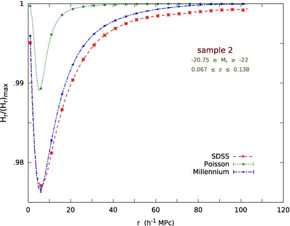
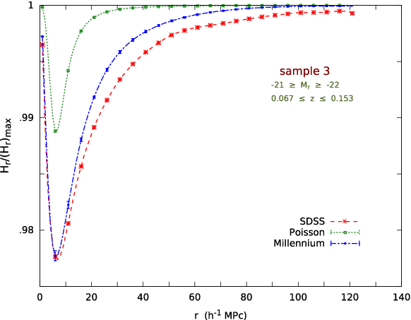
In Figure 3 we show the relative Shannon entropy at different length scales for the first SDSS samples described in Table 4 together with that from their mock counterparts from the Millennium simulation and Poisson point processes. These four different SDSS volume limited samples are constructed by keeping the brighter magnitude limit fixed at while gradually shifting the fainter magnitude limit from to in steps of . This ensures minimal differences in the clustering properties of the resulting samples while allowing us to probe different length scales due to their different volume coverages. The mock samples drawn from the Millennium simulation and Poisson processes have identical number density, volume and geometry as their respective actual SDSS counterparts. We see a characteristic dip in the relative Shannon entropy curve for all the samples at a length scale which corresponds to their mean inter-particle separations (Table 4). Further in all the panels of Figure 3 we see that the galaxy samples from both the SDSS and the Millennium have a higher degree of inhomogeneity as compared to their mock Poisson samples. These differences indicate that the galaxy samples must have extra sources of inhomogeneity other than the Poisson noise resulting purely from the discrete nature of the distributions. It is well known that galaxy distributions exhibit clustering which can be quantified by their correlation functions. Clustering acts as an extra source of inhomogeneity for the galaxy samples. Besides there could be an intrinsic inhomogeneity built in the distribution. The inhomogeneity from clustering and intrinsic inhomogeneous nature if any combine together with that from Poisson noise to produce the total inhomogeneities in the distributions. Irrespective of their nature inhomogeneities are expected to decrease with increasing length scales in presence of overlapping and confinement bias. Consequently these together makes it difficult to distinguish a real transition to homogeneity from an induced one. The transition can be confirmed easily if it takes place at a length scale where confinement bias does not dominate the statistics. For example in Figure 3 the mock Poisson samples corresponding to four SDSS samples show a transition to homogeneity in the range . Although the transitions are affected by Poisson noise on small scales still we can make a decision on the existence of a genuine transition to homogeneity. Galaxy distributions are far from a random Poisson distribution and if a scale of transition to homogeneity exist there it would possibly occur on sufficiently large scales where the confinement bias may overpower the inhomogeneities. Interestingly one can reduce the impact of confinement bias by simply choosing a volume which are less symmetric than a sphere or a cube. Although we have mentioned earlier that the geometry of the analyzed volume does not affect the relative Shannon entropy as shown in Figure 2, it could actually affect the statistics if the distribution is inhomogeneous nearly upto the largest length scale that can be probed with that volume. A volume like a rectangular slab whose two dimensions are significantly larger than the third one would make it sure that the available centres are spread across nearly the entire volume and would therefore never allows a situation where the spheres completely overlap with each other even at the largest radius. Thus if the number counts around different centres differ even slightly the relative Shannon entropy will show a deviation from . The geometry of our SDSS samples are not exactly slab like but definitely has a lesser symmetry than a spherical or cubic volume. This may enable us to detect the signature of any inhomogeneities present at the largest length scales probed by these samples. Although overlapping would be present at each scale, it may not be able to erase the inhomogeneities completely even at the largest scale due to the lesser impact of the confinement bias. Any residual inhomogeneity detected at the largest length scales are less likely to borne out of pure Poisson noise. At the largest length scale the numbers of spheres could be drastically small so we decided to consider only upto the length scales where this number reduces to . In Figure 5 we show how the number of centers vary with length scales for all the six SDSS samples analyzed here. We can see that different samples probe upto different length scales and the scale where the number of available centres reduces to for sample 1, sample 2, sample 3 and sample 4 are , , and respectively. In the top left panel of Figure 3 the relative Shannon entropy for the SDSS sample 1 clearly shows a deviation from unity at signaling some residual inhomogeneities on that scale. The results of the mock Poisson samples shown in Figure 3 indicate that for the galaxy samples having number densities comparable to our SDSS samples the contribution from Poisson noise can be safely neglected beyond . Further sample 1 being the densest of the SDSS samples analyzed here would be least affected by the Poisson noise at all length scales. This indicates that the galaxy distribution is not homogeneous on . The results from SDSS sample 2, sample 3 and sample 4 are shown in the top right, bottom left and bottom right panel of Figure 3 respectively. sample 2, sample 3 and sample 4 are , and times less denser than sample 1 (Table 4) and are expected to have a greater contribution from Poisson noise at all length scales. Interestingly the relative Shannon entropy for sample 1, sample 2, sample 3 and sample 4 are nearly same at . As sample 2, sample 3 and sample 4 probe progressively larger length scales we see that the relative Shannon entropy increases further with increasing length scales. It may appear as if the reduction in inhomogeneity with increasing length scales as revealed by progressively larger samples could result from a greater degree of overlap between the spheres. But the samples probing larger scales have larger volumes and for each of them we restrict our attention only upto a scale where the number of centers reduces to . So the degree of overlap would not vary across the samples given we limit our attention upto this specific length scale. All the four panels of the Figure 3 show that the relative Shannon entropy change very slowly on large scales indicating that the degree of overlap do not change rapidly for our sample geometries possibly due to a less aggressive confinement bias. It may be noted further that the values of relative Shannon entropy for sample 2, sample 3 and sample 4 are nearly same at and they are also same at for sample 3 and sample 4. These together clearly demonstrate the decreasing importance of Poisson noise with increasing length scales and indicate that any residual inhomogeneities at the largest length scale could be safely attributed to the presence of genuine inhomogeneity in the distribution at the corresponding length scale. We identify the transition scale to homogeneity corresponding to which the value of lies within (Pandey, 2013). This criteria is satisfied at for the sample 4. We also test if this result holds for galaxy samples having sizes bigger than sample 4 and therefore probing larger length scales. We construct another two volume limited samples namely sample 5 and sample 6 (see Table 4) which are larger than sample 4. We could not prepare the mock samples for sample 5 and sample 6 from the Millennium simulation due to the limitations arising out of the size of the simulation volume. However we analyze sample 5 and sample 6 and find that regardless of their volumes and number densities the distributions become homogeneous at . This can be clearly seen in Figure 4 where we find that the value of the relative Shannon entropy of sample 4, sample 5 and sample 6 agree within at conforming to homogeneity. Importantly there are centers available at for both sample 5 and sample 6 which reduces to at and respectively. The observed offset between the curves below the scale of may indicate the presence of a sample size dependent finite size effect. To test this we applied the same cut in the upper redshift limit of sample 5 and sample 6 as applied for sample 4 (Table 4). This ensures same volume and geometry for these samples as they have the same lower redshift limit and sky coverage. We reanalyzed the resulting samples and find that the offset between the curves persists with very little changes in the differences and all three curves finally merges at (Figure 6). The offset between the curves primarily originate from the differences in the number density and clustering in the galaxy distributions. sample 5 and sample 6 have brighter magnitude limits and lower number densities than sample 4. Poisson noise induced inhomogeneities resulting from different number densities plays an important role on small scales and become less important as the radius increases (Figure 2). Differences in inhomogeneities due to the differences in clustering may persist upto a large length scale. The fact that all three curves from sample 4, sample 5 and sample 6 reconcile at indicates that the differences in their inhomogeneities cease to exist at this length scale. The length scale where all three curves merge reduces to in this case (Figure 6). This results from the decrease in the available number of centres at all length scales when the sample 5 and sample 6 are trimmed. It may be noted in Figure 5 and Figure 7 that the number of available centers reduces from to at and for sample 5 and sample 6 respectively when they are trimmed to match with the size of sample 4.
It may be interesting to note here that an analysis of filamentarity in the Luminous Red Galaxy (LRG) distribution found that the filaments are statistically significant upto a length scale of (Pandey et al., 2011). Some recent studies (Einasto et al., 2015a; Einasto et al., 2015b) of the distribution of nearby rich galaxy clusters and superclusters in the SDSS find the evidence of shell like structures on . In different panels of Figure 3 we see that the mock galaxy samples from the Millennium simulation also does not become homogeneous at least up to a length scale of and become homogeneous at . We note that all the SDSS samples exhibit a greater degree of inhomogeneity as compared to their mock counterparts from the Millennium simulation. Nevertheless we can not deny that the complex issues of overlapping and confinement bias cast some uncertainty in the interpretations which can be resolved with yet larger samples with a reasonable number density.
In future we plan to carry out analysis with the Luminous Red galaxy distributions (LRG) (Eisenstein et al., 2001) and the Baryon Oscillation Spectroscopic Survey (BOSS) (Dawson et al., 2013) from SDSS which cover enormous volumes providing opportunities to probe much larger scales. Noticeably this would also enable us to perform the analysis with non-overlapping independent spheres even at sufficiently larger length scales. Analysis with non-overlapping spheres would have a remarkable advantage over the overlapping spheres as in the later the inhomogeneities are suppressed at each length scales making it difficult to detect them particularly at larger scales. This would help us to discern any inhomogeneities present even at the largest scales with nearly equal ease and settle the issue of cosmic homogeneity with an unprecedented confidence.
5 ACKNOWLEDGEMENT
Funding for SDSS-III has been provided by the Alfred P. Sloan Foundation, the Participating Institutions, the National Science Foundation, and the U.S. Department of Energy Office of Science. The SDSS-III web site is http://www.sdss3.org/.
SDSS-III is managed by the Astrophysical Research Consortium for the Participating Institutions of the SDSS-III Collaboration including the University of Arizona, the Brazilian Participation Group, Brookhaven National Laboratory, Carnegie Mellon University, University of Florida, the French Participation Group, the German Participation Group, Harvard University, the Instituto de Astrofisica de Canarias, the Michigan State/Notre Dame/JINA Participation Group, Johns Hopkins University, Lawrence Berkeley National Laboratory, Max Planck Institute for Astrophysics, Max Planck Institute for Extraterrestrial Physics, New Mexico State University, New York University, Ohio State University, Pennsylvania State University, University of Portsmouth, Princeton University, the Spanish Participation Group, University of Tokyo, University of Utah, Vanderbilt University, University of Virginia, University of Washington, and Yale University.
References
- Ahn et al. (2014) Ahn, C. P., Alexandroff, R., Allende Prieto, C., et al. 2014, ApJS, 211, 17
- Alam et al. (2015) Alam, S., Albareti, F. D., Allende Prieto, C., et al. 2015, arXiv:1501.00963, Accepted to ApJS
- Amendola & Palladino (1999) Amendola, L., & Palladino, E. 1999, ApJ Letters, 514, L1
- Baugh et al. (1998) Baugh, C.M., Cole, S., Frenk, C.S. & Lacey, C.G. 1998, ApJ, 498, 504
- Benson et al. (2002) Benson, A.J., Lacey, C.G., Baugh, C.M., Cole, S. & Frenk, C.S. 2002, MNRAS, 333, 156
- Biswas et al. (2010) Biswas, T., Notari, A., & Valkenburg, W. 2010, JCAP, 11, 30
- Bharadwaj et al. (1999) Bharadwaj, S., Gupta, A. K., & Seshadri, T. R. 1999, A&A, 351, 405
- Bolejko et al. (2011) Bolejko, K., Célérier,M.-N., & Krasiński, A. 2011, Classical and Quantum Gravity, 28, 164002
- Borgani (1995) Borgani, S. 1995, Physics Reports, 251, 1
- Blake & Wall (2002) Blake, C., & Wall, J. 2002, Nature, 416, 150
- Bruzual & Charlot (2003) Bruzual, G., & Charlot, S. 2003, MNRAS, 344, 1000
- Buchert & Ehlers (1997) Buchert, T., & Ehlers, J. 1997, A&A, 320, 1
- Buchert (2001) Buchert, T. 2001, General Relativity and Gravitation, 33, 1381
- Clarkson (2012) Clarkson, C. 2012, Comptes Rendus Physique, 13, 682
- Clifton et al. (2008) Clifton, T., Ferreira, P. G., & Land, K. 2008, Physical Review Letters, 101, 131302
- Cole et al. (1994) Cole, S., Aragon-Salamanaca, A., Frenk, C.S., Navarro, J.F., Zepf, S.E. 1994, MNRAS, 271, 781
- Cole et al. (2000) Cole, S., Lacey, C.G., Baugh, C.M.& Frenk, C.S. 2000, MNRAS, 319, 168
- Coleman & Pietronero (1992) Coleman, P. H., Pietronero, L. 1992, Physics Reports, 213, 311
- Colles et al. (2001) Colles, M. et al.(for 2dFGRS team) 2001,MNRAS,328,1039
- Croton et al. (2006) Croton, D. J., Springel, V., White, S. D. M., et al. 2006, MNRAS, 365, 11
- Dawson et al. (2013) Dawson, K. S., Schlegel, D. J., Ahn, C. P., et al. 2013, AJ, 145, 10
- De Lucia & Blaizot (2007) De Lucia, G., & Blaizot, J. 2007, MNRAS, 375, 2
- Eisenstein et al. (2001) Eisenstein, D. J., Annis, J., Gunn, J. E., et al. 2001, AJ, 122, 2267
- Ellis (2011) Ellis, G. F. R. 2011, Classical and Quantum Gravity, 28, 164001
- Einasto et al. (2015b) Einasto, M., Heinämäki, P., Liivamägi, L. J., et al. 2015, arXiv:1506.05295
- Einasto et al. (2015a) Einasto, M., Gramann, M., Saar, E., et al. 2015, A&A, 580, A69
- Fixsen et al. (1996) Fixsen, D. J., Cheng, E. S., Gales, J. M., et al. 1996, ApJ, 473, 576
- Gunn et al. (2006) Gunn, J. E., Siegmund, W. A., Mannery, E. J., et al. 2006, AJ, 131, 2332
- Gunn et al. (1998) Gunn, J. E., Carr, M., Rockosi, C., et al. 1998, AJ, 116, 3040
- Guo et al. (2011) Guo, Q., White, S., Boylan-Kolchin, M., et al. 2011, MNRAS, 413, 101
- Guzzo (1997) Guzzo, L. 1997, New Astronomy, 2, 517
- Hawkins et al. (2003) Hawkins, E., Maddox, S., Cole, S., et al. 2003, MNRAS, 346, 78
- Hazra & Shafieloo (2015) Hazra, D. K., & Shafieloo, A. 2015, arXiv:1506.03926
- Hogg et al. (2005) Hogg, D. W., Eisenstein, D. J., Blanton, M. R., Bahcall, N. A., Brinkmann, J., Gunn, J. E., & Schneider, D. P. 2005, ApJ, 624, 54
- Kauffmann, White & Guiderdoni (1993) Kauffmann, G., White, S.D.M. & Guiderdoni, B. 1993, MNRAS, 264, 201
- Kauffmann & White (1993) Kauffmann, G. & White, S.D.M. 1993, MNRAS, 261, 921
- Kauffmann (1996) Kauffmann, G. 1996, MNRAS, 281, 487
- Kolb et al. (2006) Kolb, E. W., Matarrese, S., & Riotto, A. 2006, New Journal of Physics, 8, 322
- Kolb et al. (2010) Kolb, E. W., Marra, V., & Matarrese, S. 2010, General Relativity and Gravitation, 42, 1399
- Kurokawa et al. (2001) Kurokawa, T., Morikawa, M., & Mouri, H. 2001, A&A, 370, 358
- Larena et al. (2009) Larena, J., Alimi, J.-M., Buchert, T., Kunz, M., & Corasaniti, P.-S. 2009, Physical Review D, 79, 083011
- Martinez & Jones (1990) Martinez, V. J., & Jones, B. J. T. 1990, MNRAS, 242, 517
- Martinez & Coles (1994) Martinez, V. J., & Coles, P. 1994, ApJ, 437, 550
- Martinez et al. (1998) Martinez, V. J., Pons-Borderia, M.-J., Moyeed, R. A., & Graham, M. J. 1998, MNRAS, 298, 1212
- Pan & Coles (2000) Pan, J., & Coles, P. 2000, MNRAS, 318, L51
- Pandey (2013) Pandey, B. 2013, MNRAS, 430, 3376
- Pandey et al. (2011) Pandey, B., Kulkarni, G., Bharadwaj, S., & Souradeep, T. 2011, MNRAS, 411, 332
- Paranjape (2009) Paranjape, A. 2009, arXiv:0906.3165
- Penzias & Wilson (1965) Penzias, A. A., & Wilson, R. W. 1965, ApJ, 142, 419
- Peebles (1993) Peebles, P. J. E. 1993, Principles of Physical Cosmology. Princeton, N.J., Princeton University Press, 1993
- Peebles (1980) Peebles, P. J. E. 1980, The large scale structure of the Universe. Princeton, N.J., Princeton University Press, 1980, 435 p.,
- Sarkar et al. (2009) Sarkar, P., Yadav, J., Pandey, B., & Bharadwaj, S. 2009, MNRAS, 399, L128
- Scharf et al. (2000) Scharf, C. A., Jahoda, K., Treyer, M., et al. 2000, ApJ, 544, 49
- Schwarz (2002) Schwarz, D. J. 2002, arXiv:astro-ph/0209584
- Scrimgeour et al. (2012) Scrimgeour, M. I., Davis, T., Blake, C., et al. 2012, MNRAS, 3412
- Shannon (1948) Shannon, C. E. 1948, Bell System Technical Journal, 27, 379-423, 623-656
- Smoot et al. (1992) Smoot, G. F., Bennett, C. L., Kogut, A., et al. 1992, ApJ Letters, 396, L1
- Somerville & Primack (1999) Somerville, R.S. & Primack, J.R. 1999, MNRAS, 310, 1087
- Springel et al. (2005) Springel, V., White, S. D. M., Jenkins, A., et al. 2005, Nature, 435, 629
- Strauss et al. (2002) Strauss, M. A., Weinberg, D. H., Lupton, R. H., et al. 2002, AJ, 124, 1810
- Straumann (1974) Straumann, N. 1974, Helvetica Physica Acta, 47, 379
- Sylos Labini et al. (2007) Sylos Labini, F., Vasilyev, N. L., & Baryshev, Y. V. 2007, A&A, 465, 23
- Sylos Labini et al. (2009a) Sylos Labini, F., Vasilyev, N. L., & Baryshev, Y. V. 2009a, Europhysics Letters, 85, 29002
- Sylos Labini et al. (2009b) Sylos Labini, F., Vasilyev, N. L., Pietronero, L., & Baryshev, Y. V. 2009b, Europhysics Letters, 86, 49001
- Sylos Labini & Baryshev (2010) Sylos Labini, F., & Baryshev, Y. V. 2010, JCAP, 6, 021
- Sylos Labini (2011a) Sylos Labini, F. 2011a, Classical and Quantum Gravity, 28, 164003
- Sylos Labini (2011b) Sylos Labini, F. 2011b, Europhysics Letters, 96, 59001
- Tomita (2001) Tomita, K. 2001, MNRAS, 326, 287
- Valkenburg et al. (2014) Valkenburg, W., Marra, V., & Clarkson, C. 2014, MNRAS, 438, L6
- White (1979) White, S. D. M. 1979, MNRAS, 186, 145
- White & Frenk (1991) White, S. D. M. & Frenk, C. S. 1991, ApJ, 379, 52
- Wilson & Penzias (1967) Wilson, R. W., & Penzias, A. A. 1967, Science, 156, 1100
- Wu et al. (1999) Wu, K. K. S., Lahav, O., & Rees, M. J. 1999, Nature, 397, 225
- Yadav et al. (2005) Yadav, J., Bharadwaj, S., Pandey, B., & Seshadri, T. R. 2005, MNRAS, 364, 601
- Yadav et al. (2010) Yadav, J. K., Bagla, J. S., & Khandai, N. 2010, MNRAS, 405, 2009
- York et al. (2000) York, D. G., et al. 2000, AJ, 120, 1579
- Zehavi et al. (2005) Zehavi, I., Zheng, Z., Weinberg, D. H., et al. 2005, ApJ, 630, 1
- Zibin et al. (2008) Zibin, J. P., Moss, A., & Scott, D. 2008, Physical Review Letters, 101, 251303