Spectral signatures of compact sources in the inverse Compton catastrophe limit
Abstract
The inverse Compton catastrophe is defined as a dramatic rise in the luminosity of inverse Compton scattered photons. It is described by a non-linear loop of radiative processes that sets in for high values of the electron compactness and is responsible for the efficient transfer of energy from electrons to photons, predominantly through inverse Compton scatterings. We search for the conditions that drive a magnetized non-thermal source to the inverse Compton catastrophe regime and study its multi-wavelength (MW) photon spectrum. We develop a generic analytical framework and use numerical calculations as a backup to the analytical predictions. We find that the escaping radiation from a source in the Compton catastrophe regime bears some unique features. The MW photon spectrum is a broken power law with a break at due to the onset of the Klein-Nishina suppression. The spectral index below the break energy depends on the electron and magnetic compactnesses logarithmically, while it is independent of the electron power-law index (). The maximum radiating power emerges typically in the -ray regime, at energies ( ) for (),where is the maximum Lorentz factor of the injected electron distribution. We apply the principles of the inverse Compton catastrophe to blazars and -ray bursts using the analytical framework we developed, and show how these can be used to impose robust constraints on the source parameters.
Keywords:
radiation mechanisms: non-thermal – -rays: general1 Introduction
The inverse Compton catastrophe is a non-linear loop of processes that is closely related to the synchrotron self-Compton (SSC) emission when electron cooling is taken into account (Longair, 2011, e.g.). If a magnetized, non-thermal emitting source, is sufficiently compact, then it is possible that the energy density of the radiated photons dominates over the magnetic one, which causes the electrons to lose energy mainly by inverse Compton scattering rather than synchrotron radiation. In such a case, a runaway process is possible: low energy (e.g. radio) photons produced by synchrotron radiation are scattered to higher energies (e.g. in X-rays) by the same relativistic electron population. As the energy density of these high energy photons is larger than that of synchrotron photons, the electrons suffer even greater energy losses by up-scattering them to even higher energies, e.g. in -rays. In turn, these have greater energy density than the X-ray photons, and so on. This runaway process leads, on the one hand, to an increase of the electron cooling rate and, on the other hand, shifts the radiated photon power from low to high frequencies. In particular, the radiated power is shifted to the -ray regime, up to energies of the order of the maximum electron energy. Pushing this idea to its limits, the non-linear loop of processes can lead to complete and very fast electron cooling and from this, the term inverse Compton catastrophe is coined.
An important concept in the study of the inverse Compton catastrophe are the multiple up-scattered photon generations. One can label the photon generations produced in the source according to how many scatterings they have undergone after production by the synchrotron process. The synchrotron photons are defined as the zeroth order photon generation to be produced in the source, which, in turn, serve as the seed photons for the first inverse Compton scattered photon generation; similarly, photons belonging to the -th generation are the seed photons for the generation. The production of such higher order photon generations can take place even if the source is optically thin to Thomson scattering, and in this case the dominant loss of photons belonging to a certain generation (with ) is the escape from the source within a crossing time (see also Björnsson & Aslaksen 2000; Tsang & Kirk 2007).
The inverse Compton catastrophe has been mainly studied in the context of compact radio sources (Kellermann et al., 1969; Readhead, 1994; Björnsson & Aslaksen, 2000; Tsang & Kirk, 2007, e.g.). It has been initially invoked to explain the observed upper limit in the distribution of brightness temperatures () from powerful extragalactic radio sources (Kellermann et al., 1969). Later it was suggested that the observed cutoff in the distribution was not related to the inverse Compton catastrophe, since the latter sets an upper limit of K, which lies above the observed cutoff (Readhead, 1994). Yet, remains a theoretical upper limit, against which the observed brightness temperatures, e.g. derived from the intra-day variability in radio cores of blazars, are still tested (e.g. Fuhrmann et al. 2008 and references therein).
The efficient cooling of non-thermal electrons due to inverse Compton scatterings has been also studied in a different context, i.e. that of unmagnetized11 1 A first analytical treatment of pair cascade in the synchrotron self-Compton model can be found in Zdziarski & Lightman (1985); the problem of pair cascades in magnetized sources has been studied also numerically, later on, by Coppi (1992). sources with high optical depths for photon-photon absorption and Compton scattering. A large volume of literature (Fabian et al., 1986; Lightman & Zdziarski, 1987; Svensson, 1987; Zdziarski, 1988; Zdziarski et al., 1990; Svensson, 1994, e.g.) deals with the problem of pair (saturated or not) cascades that are (i) initiated by absorption of high-energy photons on a soft (fixed) photon field and (ii) mediated by efficient Compton cooling of the pairs. The main goal of these studies was to determine the properties of the escaping radiation under the modification of non-thermal pair cascades and explain, among others, the universality of the observed spectral index in the X-ray spectra of active galactic nuclei (Bonometto & Rees, 1971; Rothschild et al., 1983; Kazanas, 1984; Zdziarski et al., 1990; Svensson, 1994, e.g.).
Here we consider the production of multiple photon generations due to inverse Compton scattering in magnetized, optically thin to Thomson scattering, sources, and in the regime where pair cascades are negligible. The physical setup is similar to previous studies of the inverse Compton catastrophe (Tsang & Kirk, 2007, e.g.), yet our main goals differ. These are summarized in the following: (i) study in a systematic way the transition from linear synchrotron to non-linear SSC cooling under the presence of higher order up-scattered photon generations; (ii) develop a general analytical framework that is easy to be used and can be applied to different types of sources; (iii) determine analytically the conditions, such as the electron compactness, above which the higher order SSC photon generations dominate the energetic output of the source; (iv) derive an analytical expression for the spectral index in the limit where the multi-wavelength photon spectrum is determined by higher order photon generations; and (v) use numerical calculations to back up our analytical predictions.
This paper is structured as follows. We present our assumptions and our analytical treatment in Sect. 2 and continue in Sect. 3 with a presentation of our numerical results and a comparison against the analytical predictions. In Sect. 4 we present indicative applications of the inverse Compton catastrophe in the context of high-energy emitting astrophysical sources. We conclude in Sect. 5 with a discussion of our results.
2 Analytical results
We adopt a rather abstract framework for the description of the source, according to which, the emission region of the source is assumed to be embedded in an external (fixed) radiation field, to be homogeneous and magnetized, and to contain a population of relativistic electrons, which is constantly being replenished. In this framework, we will derive (under certain simplifying assumptions) analytical expressions for the conditions leading the source in the inverse Compton catastrophe limit. For this purpose, we will take into account not only synchrotron cooling of electrons, but also cooling on synchrotron and higher order inverse Compton-scattered photons. In order to keep the analysis as general as possible, all of our results will be expressed in terms of three basic quantities: the electron, the magnetic and the external photon compactnesses, where the compactness is a dimensionless measure of the respective energy density22 2 The (dimensionless) compactness is traditionally defined as , where and are the luminosity and size of the system (Herterich, 1974). and extensively used in studies of the emission from compact sources (Zdziarski & Lightman, 1985; Svensson, 1987; Lightman & Zdziarski, 1987; Mastichiadis & Kirk, 1995, e.g.).
2.1 Assumptions
We consider a homogeneous spherical region of radius and volume that immersed in a magnetic field of strength , and moves relativistically with Lorentz factor . As the relativistic motion of the emitting region will not become central to our analysis until much later, the only reference frame of interest, at this point, is the rest frame of the emitting region, where all the following calculations will be performed.
For the purposes of the analytical treatment, we assume that mono-energetic relativistic electrons with Lorentz factor are being injected in the emission region with a constant rate , while injection of a more realistic power-law distribution will be considered in the numerical calculations. We further assume that electrons may physically escape from the emission region at the (energy independent) characteristic timescale . This is also equal to the typical timescale for adiabatic losses, at least for a spherical source expanding close to the speed of light. Electrons lose energy through synchrotron radiation and inverse Compton scattering on the internally produced synchrotron photons (SSC) and possibly, on external photons (external Compton or EC). In order to keep the analysis as general as possible, we will not specify the origin of the external radiation until much later (Sects. 2.3 and 4). The only property of the external photon field that is currently important for our analysis is its energy density as measured in the rest frame of the emitting region.
We also approximate the emissivity of synchrotron and inverse Compton scattering by a -function centered at (dimensionless) photon energies and , respectively. Here, is the energy of a photon that has been Compton up-scattered -times, with being the comoving magnetic field strength and G. Finally, in the analytical treatment we consider only optically thin to synchrotron self-absorption (ssa) cases (see Tsang & Kirk 2007, for the role of ssa in Compton catastrophe cases).
2.2 Steady-state solutions of the electron kinetic equation
The evolution of the electron distribution is described by the kinetic equation
| (1) |
where and are the injection and energy loss operators for electrons, respectively. These are defined as
| (2) | |||||
| (3) |
where is the Heaviside function and is the total energy density. This is given by
| (4) |
The last term takes into account the energy density of successive SSC photon generations, starting from the first one () that is the result of the synchrotron photon up-scattering () and terminating at the photon generation. These photons are, in turn, the seeds for the last SSC generation to be produced in the Thomson regime. SSC photons belonging to the -th generation appear in the electron’s rest frame with energy , and thus, their up-scatter will take place in the Klein-Nishina regime, where the cross section for scattering is greatly suppressed. This also explains the absence of from the electron cooling term. The highest order of up-scattered photons in the Thomson regime, , is given by
| (5) |
where the square brackets denote the closest (from below) integer value of the enclosed expression (see Appendix A for the derivation).
In principle, one should also include in the equation of a term related to the repeated inverse Compton scatterings of external photons, similar to the last term of the r.h.s. in eq. (4). It can be shown, however, that for and typical values for the energy of external photons (e.g. 1 eV), even the first inverse Compton scattering of the EC photons takes place deep in the Klein-Nishina regime (see Appendix B). In this case, one can safely ignore the term related to the energy density of EC photons. However, this does not apply if the injected electrons are less energetic, e.g. their Lorentz factor is . Thus, for completeness reasons, we derive in Appendix B similar relations and constraints to these presented in the following paragraphs (Sects. 2.2.1-2.2.2) after including in eq. (4) the energy density of the once EC scattered photons (). The interested readers can compare how the inclusion of alters the results presented in Sect. 2.
At this point, it is useful to introduce the compactness of the magnetic and photon fields that appear in eq. (4). We define the compactness of a field, which is a dimensionless measure of its energy density, as
| (6) |
where the subscript takes the values ‘B’ (magnetic field), ‘ex’ (external photon field), ‘syn’ (synchrotron photons) and ‘ssc,i’ (-th generation of SSC photons). Similarly, one can define the injection compactness of electrons, which is given by
| (7) |
In most astrophysical applications, the total energy density is dominated by the first two or three terms, namely by the energy density of synchrotron photons and that of the magnetic field (or of ambient photon fields). In such cases, analytical time-dependent solutions of eq. (1) can be found (see Kardashev 1962; Zacharias & Schlickeiser 2010; Zacharias & Schlickeiser 2012). However, if becomes comparable33 3 We will quantify this statement in Sects. 2.2.1-2.2.2 to the sum of the first three terms, then even the derivation of steady-state solutions of eq. (1) becomes challenging, as the energy density of each SSC generation depends on itself. In such a case, one can still derive analytical steady-state solutions of eq. (1), but only in two limiting regimes, depending on which is the dominant term in the kinetic equations.
In order to define the aforementioned regimes, we introduce the ratio of the cooling and escape timescales of electrons with Lorentz factor :
| (8) |
where is defined accordingly to eq. (6).
We distinguish between two regimes44 4 We caution the reader that the slow and fast cooling regimes defined here are, strictly speaking, valid only asymptotically, i.e. for and .:
- •
If , then electron cooling is negligible and the steady-state electron distribution is determined by the balance between the escape and injection processes. The steady-state electron distribution is then simply or equivalently . Borrowing the terminology from GRBs, we will refer to this regime as slow cooling regime (see e.g. Sari et al. 1998).
- •
If , then electron cooling becomes important. In this case, the cooling Lorentz factor of electrons, which is defined by , is smaller than the injection one () and the steady-state electron distribution has the well-known power-law distribution (for mono-energetic injection), i.e. , for ; this corresponds to the so-called fast cooling regime (e.g. Piran 2004).
The normalization factors and , whose explicit form is presented in the following paragraphs, depend on the injection rate and on the energy densities of the various fields. In the paragraphs that follow, we will determine the slow and fast cooling regimes, and present the respective analytical expressions for the compactnesses .
2.2.1 Solutions in the slow cooling regime
In the slow cooling regime and for an energy independent escape timescale, the steady-state electron distribution has the same energy dependence as the source function and the normalization depends only on the injection rate as . Using the definition of eq. (7) we may write
| (9) |
The synchrotron and -th generation SSC compactnesses are written as
| (10) | |||||
| (11) |
where we used eqs. (9), (81) and (84) (see Appendix A for more details). The above expressions demonstrate the well-known linear and quadratic dependence of the synchrotron and first SSC components on (e.g. Bloom & Marscher 1996). Since , a cubic relation between the synchrotron and second SSC photon components is expected, which might be of interest for flaring events in high-energy emitting blazars (Aharonian et al., 2007).
For , expressions eqs. (10) and (11) suggest that , and the total compactness of the source, in this case, is . The spectral energy distribution (SED) of the source will be synchrotron dominated if and EC dominated, otherwise.
The compactness of successive SSC photon generations will become progressively higher, namely the source may enter the inverse Compton catastrophe regime, only if . In this case, the following ordering among the compactnesses holds:
| (12) |
The total compactness is, in a good approximation, given by
| (13) |
Depending on the relative ratio of the two terms appearing above, the SED is expected to be dominated either by the EC component or by the highest order SSC generation. Thus, even for an external photon field with high compactness, the production of higher order, and progressively more luminous, SSC photon generations cannot be suppressed for a sufficiently high electron compactness, namely . This will be demonstrated in more detail with numerical results in Sect. 3.
The results we derived so far are valid as long as the assumption of slow cooling is valid, and as such an a posteriori check is necessary. The expressions (9)-(13) are valid as long as or equivalently , where is given by
By combining the above, we find that the slow cooling solutions are valid, if the parameters satisfy the following conditions:
| (18) | |||||
| (19) |
or
| (20) | |||||
| (21) |
where
| (22) |
The quantity characterizes the relative strength of the external photon energy density relative to the magnetic field energy density, and as such the importance of EC relative to synchrotron and SSC emission. It is one of the two parameters that we use to characterize the relevant parameter phase space. Relations (18)-(19) and (20)-(21) can be used to define two distinct regions in the slow cooling parameter space. We will refer to them as and , respectively.
2.2.2 Solutions in the fast cooling regime
In the fast cooling regime the steady-state equation of electrons is written as
| (23) |
An Ansatz for the solution of the above equation is . By substituting it in the above equation we find that and that satisfies the following algebraic equation
| (24) |
where
| (25) |
Given that there is no general formula for the roots of a polynomial with degree higher than four, which corresponds to , explicit solutions of eq. (24) can be found in limiting cases only, which we list below.
- •
Synchrotron and inverse Compton cooling (on synchrotron and external photons)
The main energy loss channels for electrons are synchrotron cooling and inverse Compton scattering on external and synchrotron photons, i.e. . In this case, satisfies a second degree polynomial equation, which has the solution(26) The above expression for simplifies into the one obtained for SSC electron cooling (see also Petropoulou et al. (2013)). Using eqs. (6) and (81), we find the synchrotron photon compactness to be
(27) while the compactness of -th SSC generation is simply
(28) Expressions (27) and (28) demonstrate how the inclusion of electron cooling affects the dependence of the photon compactness of various components on the injected electron luminosity. For example, the synchrotron luminosity does not depend linearly on as in the slow cooling regime (Bloom & Marscher, 1996, e.g.), unless .
We remind the reader that the expression for was derived under the assumption of (see also eq. (24)) that allowed us to drop the sum over the energy densities of higher-order SSC photons. The condition translates into the following constraint
(29) - •
Cooling on higher order SSC photon generations
Here we consider the case where the system is driven in the Compton catastrophe regime and the dominant energy density is . The energy density of external photons may dominate over that of SSC photons, unless(30) In this limit, the solution of eq. (24) is given by
(31) The above expression is valid as long as the condition (30) holds, or equivalently if
(32) where we substituted expression (31) into eq. (30). This is the second constraint that we derive in the fast cooling regime.
Using the same equations from the Appendix A as before, we find that
(33) (34)
Before closing this paragraph we complete the set of constraints for the fast cooling regime. For this, we require the condition or to hold. Using the adequate expression for the total source compactness, i.e.
we find the following constraints:
| (38) |
or
| (39) | |||||
| (40) |
Similar to what we found for the slow cooling regime, the constraints (38) and (39)-(40) divide the fast cooling parameter regime into two sub-regions. We will refer to them as regions and , respectively.
We derived the conditions that result in the dominance of the inverse Compton emission over the synchrotron one, both in the slow and fast cooling regime. All the conditions were expressed, so far, in terms of the various compactnesses that describe the source. The strength of the inverse Compton emission is traditionally expressed also in terms of the Compton parameter (Rybicki & Lightman, 1979). For completeness, we present the relation between the Compton parameter and the various compactnesses in Appendix C. The interested reader can use this relation to express all the analytical expressions derived in Sect. 2 in terms of the parameter.
2.2.3 The parameter space
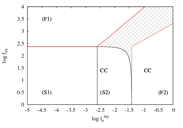
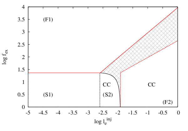
The regimes defined in the previous paragraphs are illustrated in Fig. 1, where we plot against for and two values of the magnetic compactness, i.e. (left panel) and (right panel). For a given , translates into a value of , and thus, from the plot one can read the values of all the basic compactnesses that describe the source. For the source is found to be optically thin to Thomson scatterings, where our analysis is valid (see also Sect. 3.3).
On both plots, there are some regions marked as and , which were respectively defined in Sections 2.2.1 and 2.2.2. To demonstrate the regions of the parameter space where the inverse Compton catastrophe occurs, we used the abbreviation C.C.. The dashed and solid black lines correspond to the slow cooling regime constraints of eqs. (18)-(19) and (20)-(21), respectively. The constraints obtained in the fast cooling regime, which are given by eqs. (38) and eqs. (39)-(40) are shown with solid and dashed red lines, respectively. Finally, the transition region between the two limiting cases in the fast cooling regime (see Sect. 2.2.2), is not tractable by analytical means.
The main conclusions drawn from Fig. 1 are summarized below:
- •
for a fixed , the system may enter the fast cooling regime either for high values of (lower right region) or high external photon compactnesses (upper left and middle regions). In the region , the main channel of electron energy losses is synchrotron radiation and EC scattering. In fact, there is a transition from synchrotron to EC scattering cooling, as one moves towards higher values of within the region.
- •
in the region, electrons lose energy preferentially by the SSC process. Moreover, the energy density of higher order SSC photon generations becomes larger, and as such, it dominates the total energy density which appears in the electron cooling term.
- •
the regions and of the slow cooling regime occupy the lower left and middle part of the parameter space, where both the electron and external photon compactnesses are low/moderate.
- •
the inverse Compton catastrophe may occur either in the slow cooling or in the fast cooling regimes. Higher values of are required in the latter.
- •
- •
an increase of results in a more extended fast cooling regime, as expected (see e.g. regions in the left and right panels of Fig. 1).
- •
the minimum , which is required for the inverse Compton catastrophe to occur while in the fast cooling regime, decreases as .
2.3 Observed luminosities
Having investigated the different regimes of the available parameter space, we proceed with the calculation of observed quantities, and in particular, of the bolometric synchrotron and SSC luminosity. For a spherical region moving relativistically with a Doppler factor , where is the bulk Lorentz factor and is the angle between the beaming direction and the line of sight to the observer, the observed synchrotron and SSC luminosities are easily derived by the respective compactnesses as:
| (41) |
where is given by eqs. (10)-(11) for the slow cooling regime and by eqs. (27)-(28) and (33)-(34) for the fast cooling regime. From this point on, all quantities noted with the subscript ‘obs’ will refer to the observer’s frame, while quantities with an asterisk () will be measured in the rest frame of the central engine/galaxy.

The details about the external source of photons, such as its geometry and spectral energy distribution, were not important for the derivation of the results presented in Sect. 2.2. Before stepping into the calculation of the EC observed luminosity, it is, however, useful to specify the so far arbitrary source of external photons. We consider the case of an isotropic (in the galaxy rest frame), monochromatic photon field with a photon energy and spherical geometry with a radius (see Fig. 2). Its energy density is , where is its luminosity. If the emission region is embedded in the external photon field, the energy density and the characteristic photon energy of this field in the comoving frame of the emission region appear as and , respectively (Dermer & Schlickeiser, 1993; Dermer, 1995). If, however, the emission region is located at a distance and is moving away from it with a Lorentz factor such that (see e.g. Fig. 2), the external energy density will be then significantly (by a factor of ) de-boosted (e.g. Dermer 1995). In this case, the system can be satisfactorily studied by taking into account only the internally produced photons. Finally, for cases where the boosting effect on the energy density and typical photon energies of the external radiation field will be intermediate.
For the observed EC luminosity () we follow the approach by Dermer (1995) – henceforth D95, since the external photon field in the comoving frame of the emission region is not isotropic. For the slow cooling regime, where the stationary electron distribution is mono-energetic, i.e. , we start with eq. (5) of D95 and derive (see Appendix D for more details) the observed flux due to EC scattering
| (42) |
where , is defined as
| (43) |
where and is given by
| (44) |
After integrating eq. (42) over and making the approximations , , and we find
| (45) |
For the fast cooling regime, where the stationary electron distribution is a power-law, we can use directly eq. (7) in D95. After making the substitutions and , where , we integrate eq. (7) over energies up to , and by making the same approximations as before, we derive a similar expression to that of eq. (45):
| (46) |
Thus, depends on the cooling regime only through the factors and .
For the expressions regarding the slow cooling regime we made use of eqs. (9)-(11), (41), and (45), whereas for the fast cooling regime we used eqs. (26)-(28), (33)-(34), (41), and (46). Our results are summarized below.
- -
Slow cooling regime
(47) (48) (49) - -
Fast cooling regime
In Section 2.2.2 we derived explicit expressions for the compactness of various components for two limiting cases:-
Synchrotron and inverse Compton cooling on synchrotron and external photons
(50) (51) (52) -
Cooling on higher order SSC photon generations (CC limit)
(53) (54) (55)
-
We remind the reader that the above expressions are strictly valid in the slow (regions ) and fast (regions ) cooling regimes, and one should use them with caution for parameters falling in the transition regime (e.g. hatched regions in Fig. 1).
2.4 Photon spectrum in the CC limit
Besides the observed luminosity of the various components that build the multi-wavelength spectrum in the Compton catastrophe regime, we are also interested in the spectral shape. As already described in Sect. 1, the inverse Compton catastrophe refers to the case where higher order SSC photon generations are progressively more luminous, i.e. . The ordering of the emitting components in terms of their luminosities, with the synchrotron component being the least luminous, implies that the photon spectrum will be a power-law, defined by the peaks of successive components, which will extend up to an energy MeV (as measured in the comoving frame).
Being equipped with all the necessary analytical expressions, we can turn now to the spectral index, , (approximating the photon spectrum as a power-law, i.e. ) in the Compton catastrophe limit. Assuming that the bolometric luminosity of each component is a good proxy for the peak luminosity, we can estimate through the approximate relation
| (56) |
where . Using eqs. (48) and (54) for the slow and fast cooling regimes, respectively, we find
Equation (2.4) reveals the dependence of the spectral slope on various physical parameters. For example, in the fast cooling regime, a decrease of the magnetic field strength and/or of the size of the emission region, results in lower values, and thus, tends to make the photon spectrum harder (smaller values). Notice that is independent of the magnetic compactness in the slow cooling regime, while higher lead to harder photon spectra in both regimes. In principle, there is no lower limit on . However, very hard photon spectra with would require unphysically large due to the logarithmic dependence on the latter. In any case, our results cannot be extended to , since in this parameter regime other processes, such as photon-photon absorption and pair cascades, become important and they cannot be neglected anymore.
The spectral index given by eq. (2.4) is obtained for parameters drawn from the sub-regions and in the parameter space. This is exemplified in Fig. 3, where we adopted and . In the fast cooling regime, the Compton catastrophe photon spectra tend to be harder than these of the slow cooling regime. Figure 3 demonstrates also that the spectra in the Compton catastrophe limit become harder as increases. However, because of the weak logarithmic dependence on (see color bar), very high values of are required for . Finally, we note that a choice of a lower would not have a strong impact on (see eq. (2.4)), but it might affect the extend of the sub-regions and .

3 Numerical results
The results presented in the previous section were derived by solving the simplest form of the electron kinetic equation (see eq. (1)) and by using a series of approximations. In this section, we present the results of a numerical treatment of the problem, which does not suffer from the simplifying assumptions used in Sect. 2, albeit its own limitations. Our aim is to test whether or not these simplifications have a radical effect on the results regarding the transition to the Compton catastrophe regime, as well as the multi-wavelength spectral properties in this limit.
The numerical treatment of the problem allows us to augment the relativistic electron kinetic equation with more processes, such as pair injection due to photon-photon absorption, and to make use of the full expressions for the synchrotron and Compton emissivities in the relativistic limit. In addition, we write an accompanying equation for photons, which is coupled to the one for electrons. The physical system is then described by
| (61) | |||||
| (62) |
The various terms appearing above describe the following physical processes: (i) Photon-photon pair production, which acts as a source of new particles () and a sink term for photons (); (ii) synchrotron radiation, which acts as an energy loss term for electrons () and a source term for photons (); (iii) synchrotron self-absorption, which acts as a sink term for photons (); and (iv) inverse Compton scattering, which acts as an energy loss term for electrons55 5 Both external and internal photons serve as targets for the inverse Compton scattering process. () and an energy injection term for photons () The escape timescale for electrons is set equal to the crossing time of the source, i.e. . Note that the expressions for the synchrotron and Compton emissivities in the relativistic limit (c.f. eqs. (6.33) and (2.48) in Rybicki & Lightman (1979) and Blumenthal & Gould (1970a), respectively) have been used in eq. (62). For more details about the functional forms of the various rates, see Appendix E.
Synchrotron self-absorption is taken into account only as a sink for photons, while there should be an additional source (heating) term for the electrons. Although this is not, strictly speaking, an energy conserving scheme, in all cases we present the absorbed energy by synchrotron self-absorption is small, and electron heating can be neglected. Equations (61) and (62) could not be applied in their present form in the “synchrotron boiler” case, where (Ghisellini et al., 1988).
As the numerical code makes no distinction between electrons and positrons (both determined by eq. (61)), the treatment of the pair annihilation in the code is approximate (Coppi, 1992, see e.g.). As long as we consider optically thin cases, i.e. (or, equivalently where is the Thomson optical depth and is defined in Appendix C) the pair yield is very low and the annihilation can safely be neglected. The annihilation line starts becoming important for (Lightman & Zdziarski, 1987, e.g.), where our numerical approach becomes invalidated.
In summary, the numerical code used in this paper and presented originally in Mastichiadis & Kirk (1995) is adequate for the description of system containing relativistic electrons () with compactnesses up to . Exploration of a system containing electrons with and/or with very high compactness requires more sophisticated numerical treatment (Coppi, 1992; Stern et al., 1995; Belmont et al., 2008; Vurm & Poutanen, 2009, e.g.); this, however, lies out the scope of the present study.
3.1 Comparison with analytical results
As a first step, we compare the analytically derived values for the observed luminosities (see Sect. 2.3) against the values we obtained by numerically solving eqs. (61) and (62), without including the terms of synchrotron self-absorption and photon-photon absorption. In this way, we ensure that any differences found between the numerical and analytical results will have to be related with the simplifying approximations of the analytical treatment and not with the physical processes themselves.
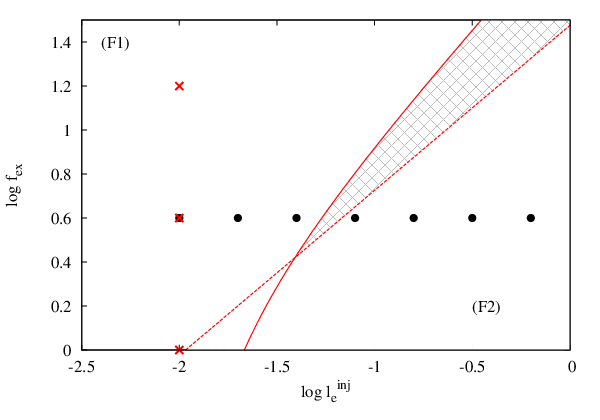
For the comparison we adopted the fiducial parameter set of , , G, cm, . Substitution of the and values in eq. (5) results in . The magnetic compactness is found to be . To test the effect of the external photon field on electron cooling and on the multi-wavelength photon spectra we used three indicative values for its compactness, namely and , which correspond to equally spaced values of . In all cases but , the basic compactnesses are ordered as . For the characteristic energy of external photons, we used the fiducial value eV.
Using the analytical expressions of eqs. (18)-(21) and (38)-(40) we construct the respective parameter space, which is illustrated in Fig. 4. The parameter values adopted for the comparison are shown as red crosses. For all three values of , we analytically predict that the system should lie in the fast cooling regime (sub-region ). We note that even for , the magnetic compactness () is high enough as to make the injected electrons cool efficiently. This is indicated by the absence of the slow cooling regions in Fig. 4. In what follows, we will compare the aforementioned predictions with the respective numerical results.
First, we verified that the steady-state electron distribution is described by as a result of efficient cooling, for all values of . The multi-wavelength photon spectra calculated numerically for the three values of are shown in Fig. 5. Photon spectra obtained for and are plotted with black, red and blue lines, respectively. The synchrotron and inverse Compton components of the total emission (thick line) are plotted with dashed and dotted lines, respectively. For illustration reasons, the external radiation field is not shown. The flux values marked on the right vertical axis correspond to a source placed at redshift .
In agreement with our analysis, we find two SSC photon generations being produced in the Thomson regime. This is evident in the case of pure SSC emission (black lines). The increase of has two effects on the shape of the SED. On the one hand, the synchrotron luminosity decreases, while, on the other hand, there is a transfer of power from the SSC to the EC component (see e.g. red and blue lines in Fig. 5). This reflects the transition from synchrotron cooling to cooling due to EC scattering, which is in agreement with the analytical predictions (see Sect. 2.2.3).
Apart from a qualitative comparison, we can compare the bolometric synchrotron, SSC and EC luminosities as derived numerically and analytically from the appropriate expressions in Sect. 2, namely using eqs. (50)-(52). The results are listed in Table 1. In all cases, the analytically derived values do not differ more than a factor of from those derived numerically. Given the simplifying assumptions we used to derive the analytical expressions in the first place, we argue that the results are in good agreement to each other.

| A(a) | N(b) | A | N | A | N | |
| (erg/s) | ||||||
| (erg/s) | ||||||
| (erg/s) | hidden(c) | hidden | ||||
| (erg/s) | – | – | ||||
- a
- b
Calculated numerically – see also Fig. 5.
- c
The numerical code cannot distinguish between photons with EC and SSC origin, if they are produced at the same energy range. For example, if , the 2nd SSC photon generation will be hidden by the EC one. Thus, we cannot numerically calculate its luminosity.
3.2 Transition to the inverse Compton catastrophe
In this paragraph we demonstrate the modification of the multi-wavelength photon spectra caused by a gradual increase of the electron injection compactness, which eventually leads the source to the Compton catastrophe regime. Same as in previous paragraph, we neglect the effects of additional processes, such as synchrotron self-absorption, which will be discussed separately in a following paragraph.
We use as a starting point, the fiducial parameter set of the previous section with (see Fig. 4). In this case, the external photon energy density is the dominant term in the electron cooling. This is also reflected to the SED shown in Fig. 5, where most of the bolometric photon luminosity is carried by the EC component. We will show next that even in this case, higher order SSC photon generations may have a dominant contribution to the SED and electron cooling, for sufficiently high , as already pointed out in Sect. 2. Since this particular example falls in the fast cooling regime, we can use the expressions for and given by eqs. (54) and (55), respectively, in order to predict the necessary electron compactness for the highest SSC component to be the most luminous. By demanding , we find that , yet .
We initiate the numerical calculations with and keep increasing by a factor of two over its previous value until we reach . The predicted value for the transition to the inverse Compton catastrophe is slightly below the maximum value used in the simulation ( in logarithm). The successive values are shown as black circles in the parameter space of Fig. 4.

The successive photon spectra are shown in Fig. 6 with solid lines, while spectra obtained for the pure SSC case, i.e. with , are shown with dashed lines for comparison reasons. For the particular choice of parameters (see also Fig. 5), we find that the EC emission dominates in the -rays, while the SSC emission is being suppressed, for low enough values of the electron compactness, i.e. . As the electron compactness progressively increases, however, the contribution of the EC component to the high-energy part of the spectrum becomes less significant. We find, in particular, that it is the second SSC emission that actually dominates the multi-wavelength emission for (second spectrum from the top). Note that this value is in good agreement with the analytical estimate derived above. Finally, the spectrum obtained for is a typical example of emission in the Compton catastrophe regime (Björnsson & Aslaksen, 2000, see also Fig. 2 in) and bears several ‘generic’ features:
- 1.
The bulk of the total luminosity is emitted at the high-energy part of the spectrum. For the pure SSC case shown in Fig. 6 (dashed lines), the SED peaks at approximately MeV or Hz. As already mentioned in Sect. 2.2, the succession of higher than SSC photon generations ceases due to the Klein-Nishina effects. The highest energy of the inverse Compton scattered photons should be For the values numerical example of Fig. 6, we find GeV or Hz. Notice the abrupt cutoff of the photon spectra at this frequency.
- 2.
The SED shows smooth spectral breaks at the transition between successive emission components. This effect is evident, if the electron distribution is mono-energetic or spans over a narrow range of energies. However, for a power-law electron distribution with index , the spectral breaks are smoothened out (see next section).
- 3.
For even higher compactnesses, namely , we verified that the spectrum tends to be a power-law with spectral index . This is in agreement with the analytical estimate of eq. (2.4), but it will become more clear with the numerical examples that follow (Sect. 3.2.1).
We have shown that there is a general agreement between the analytical and numerical results regarding the electron cooling regimes, the luminosities of the various components, the transition of the system to the Compton catastrophe regime, and the respective spectral shape in the Compton catastrophe limit. There are, however, several factors that might affect the spectral index , such as the distribution of electrons at injection (mono-energetic versus power-law) and photon-photon absorption, which redistributes the energy from the high-energy part of the spectrum to lower energies through an electromagnetic cascade. As the analytical treatment has its limitations, in what follows, we investigate the role of these factors numerically for a pure SSC case ().
3.2.1 Effects of the electron power-law index
So far, we have presented multi-wavelength spectra obtained for mono-energetic injection of electrons. However, the spectral index may depend on the power-law shape of the electron distribution at injection. To test this hypothesis, we consider here the case of a power-law injection of electrons (with ) i.e. , with , . We use three indicative values for the power-law index () that correspond to electron energy spectra ranging from soft to hard. For each case, we calculated the spectral for five values of the injection compactness starting with , and increasing over its previous value by in logarithm. Other parameters used are: G, cm, leading to . In order to isolate the effects that a different power-law index has on the photon spectra, we artificially switched off the terms related to photon-photon absorption and synchrotron self-absorption from eqs. (61) and (62).


The results for and 1 are presented in the top, middle and bottom panels of Fig. 7. In all cases, we show the total (synchrotron and inverse Compton) emission in terms of photon compactness. Different types of lines correspond to different marked on the plot. In all cases the steady-state electron distribution has cooled efficiently down to .
For low enough electron compactnesses, we recover the well known result (Blumenthal & Gould, 1970b, e.g.) that the spectral shape of the SED depends on the power-law index of the electron distribution (see e.g. spectra for in all panels of Fig. 7). However, as the system is pushed in the Compton catastrophe regime (), the SEDs obtain a broken power-law shape with a break at as measured in the comoving frame. The spectral index below the break energy is universal, in the sense that, it is no more related to the power-law index of electrons at injection, but depends only on and (for a discussion on the characteristic Lorentz factor in the case of power-law injection, see Björnsson & Aslaksen (2000)). However, the photon spectra for (comoving energies) are steep and their spectral index is related to the power-law index of electrons at injection. The broken power-law shape and the steepening of the spectrum above the break energy are both results of the Klein-Nishina cutoff effect (for a relevant discussion, see Zdziarski & Lamb (1986)). We note that the spectra above the high-energy break should appear even steeper, had the photon-photon absorption be taken into account, while would be marginally affected by the development of pair cascades (see Sect. 3.3).
The numerically derived values of , whenever they can be defined, are marked on the plot, and are in relative agreement with the value derived by eq. (2.4). Moreover, we find that the photon spectra in the Compton catastrophe regime become harder as the electron compactness increases. In particular, a one order of magnitude increase in leads to a larger by 0.12 units. The weak dependence of on is in full agreement with the analytical prediction (see eq. (2.4)). On the contrary, a one order of magnitude change in , before the source enters the Compton catastrophe regime, results in significant changes of the photon spectral shape (see Fig. 7). The sensitivity of the multi-wavelength photon spectra on , before and after the transition to the Compton catastrophe regime, is also reflected by the different density of curves in the panels of Fig. 7 as increases.
It is noteworthy that the photon spectra we obtain in the Compton catastrophe regime are not as hard as those predicted by Zdziarski & Lamb (1986), which have a spectral index for even lower values of the electron compactness. After excluding a numerical error as the reason of this discrepancy (see Appendix F), we argue that the hardness of the photon spectra in the Compton catastrophe regime depends also on the nature of the seed photons used in the scatterings. Here, we study the effects of repeated inverse Compton scatterings of the synchrotron photons by relativistic electrons, whereas Zdziarski & Lamb (1986) considered a fixed black-body photon field.

3.3 Effects of additional processes
We turn now to discuss additional processes that were not included so far and can influence the system.
- 1.
Synchrotron self-absorption: for the parameter regime we are interested in, this process acts as a loss term for low-energy photons (see eq. (62)) and reduces the number density of synchrotron photons, which are the targets for the first SSC photon generation. It may, therefore, affect the spectral slope in the Compton catastrophe regime. In order to test this, we calculated numerically the steady-state photon spectra for the same cases shown in Fig. 7; the case of is exemplified in Fig. 8. In general, inclusion of synchrotron self-absorption makes the multiple SSC components more pronounced for low , while in the Compton catastrophe regime the spectrum is characterized by smaller . Qualitatively speaking, this is expected, since synchrotron self-absorption removes low-energy photons that would be, otherwise, multiply up-scattered and contribute to the high-energy emission of the source. Quantitatively though, the effect is not significant, since in all cases changed no more by a factor of 0.1-0.2. For example, for and (Fig. 8) we obtain instead of 0.9 after the inclusion of synchrotron self-absorption.
- 2.
Photon-photon absorption: inclusion of this process, makes the high energy part of the spectrum, i.e. at , steeper. This is exemplified in Fig. 9, where we show the photon spectra for and calculated with (dashed lines) and without (solid lines) photon-photon absorption. For each value of , we plot the spectra for and 1 are (from bottom to top). Only for and starts photon-photon absorption to have a significant impact on the high-energy part of the spectrum. Note, however, that the injected secondary pairs do not modify the spectrum below the break. This becomes important only for (Svensson, 1994, see e.g. Fig. 2 in). In short, for the parameter regime where our analysis is valid the effects of photon-photon absorption are minimal.
Finally, other processes that might be important in optically thick plasmas such as photon down-scattering on electrons, electron-positron annihilation, Coulomb collisions and bremsstrahlung turn out to be negligible as the Thomson optical depth in all our cases is always much less than unity.
4 Relevance to astrophysical sources
We have shown that the multi-wavelength photon spectra in the Compton catastrophe regime obtain a universal power-law shape that peaks at observed energies , where most of the power is emitted. In contrast to the photon spectra obtained for low values of the electron compactness, where one can link the observed spectral index with the power-law index of the electron distribution, in the Compton catastrophe regime this connection can no more be established. The same applies for the EC emission, which for high enough is hidden below the higher order SSC components. These properties make the photon emission in the Compton catastrophe unique.
For the derivation of the analytical relations presented in Sect. 2, we adopted the most general framework as possible, i.e. we did not attempt to specify the astrophysical source. The results regarding the observed bolometric luminosities of the various spectral components are obtained for an emitting region that is relativistically moving towards the observer and is embedded in a spherical and isotropic (in the rest frame of the galaxy) external photon field. These analytical relations are valid as long as the relations and hold. In this section, we apply the analytical results of Sect. 2 to the high-energy emitting region of either a blazar jet or a GRB jet.
4.1 Blazar emission
Assuming that the blazar multi-wavelength emission (from the infrared (IR) wavelengths up to -ray energies) arises from one region, then the observed spectrum cannot be reconciled with that expected in the inverse Compton catastrophe limit. One example is the absence of an excessively high X-ray flux from radio-loud blazars, whose radio cores exhibit extreme apparent brightness temperatures. This may exclude the possibility of a source being in the inverse Compton catastrophe limit (e.g. Ostorero et al. 2006; Agudo et al. 2006). If, however, the one-zone assumption proves to be wrong, i.e. the IR-optical and -ray emission are produced in different locations, then it is still possible to explain the high-energy emission in terms of a non-thermal pair cascade (Stern & Poutanen, 2006; Stern & Poutanen, 2008, e.g.).
In the following, we adopt the one-zone framework for the blazar emission, and, as an indicative example, we focus on blazars whose -ray emission is dominated by the EC component. Thus, what follows may be of relevance for flat spectrum radio quasars (FSRQs) and low-frequency peaked BL Lacs (e.g. 3C 273 and BL Lacertae). In the fiducial example of Fig. 6 we showed that, for sufficiently high , the emission from the highest order SSC photon generation may dominate that of EC component. Thus, in the case of EC dominated blazar emission, it is interesting to search for the conditions that suppress the emission from highest order SSC photon generation, and derive information about the properties, e.g. size and luminosity, of the external radiation field.
We present the results for the fast cooling case, since it is the regime that ensures high radiative efficiency. The luminosity ratio between the high- and low-energy components of the blazar SED is usually referred as the Compton dominance of the source. In cases where the EC component dominates the emission in high-energies (X-rays up to -rays) the ratio is defined as (e.g. Sikora et al. 2009) or . The condition results in
| (63) |
where we used eqs. (54) and (55). Using the constraint of eq. (40) we find that
| (64) |
which when combined with the relation (63) results in with given by
| (65) |
where is the Lorentz factor of the emission region. In the above, we introduced the notation in csg units, unless stated otherwise. We also assumed that the source of the external radiation is the reflected blazar’s disk luminosity () at the broad line region (BLR). The latter, for the purposes of this study, was taken to be spherical with radius (see also Fig. 2). In the derivation of (65) we, thus, assumed and used and erg/s as typical values (see e.g. Böttcher et al. 2013; Nalewajko et al. 2014).
Relation (65) shows that the inverse Compton catastrophe may be avoided, if the external source of radiation, the BLR in our case, has a sub-pc scale size ( pc)66 6 Interestingly, the BLR radius is typically found to be pc (see Nalewajko et al. 2014, and references therein).. For a given , a pc-scale BLR on the other hand, is dilute enough as to favour the SSC emission and even lead the source to the Compton catastrophe limit for sufficiently high . In general, the upper limit we derived for becomes even more stringent for lower reflection efficiencies and less luminous disks. Although a larger emission region and/or the injection of electrons with higher Lorentz factors, push the upper limit close to the pc-scale, the dependence of on both parameters is relatively weak ().
The aforementioned results suggest that the inverse Compton catastrophe does not typically occur in these sources. Before closing this paragraph we note that higher order SSC photon generations () may become relevant for -ray emitting radio galaxies, such as Cen A and M 87, even if the sources are not in the extreme regime of the Compton catastrophe. In the particular case of Cen A, Petropoulou et al. (2014) studied in detail the role of the second SSC photon generation on the high-energy emission detected from the core of Cen A.
4.2 GRB emission
Amongst the various proposed mechanisms for the GeV emission of GRBs77 7 Although the GRB GeV emission became a topic of interest after the Fermi-LAT detections (Ackermann et al., 2013), it has been already observed with CGRO/EGRET (Hurley et al., 1994; González et al., 2003). , the inverse Compton scattering has been discussed in several studies (Dermer et al., 2000; Guetta & Granot, 2003; Granot & Guetta, 2003; Pe’er & Waxman, 2004; Beloborodov, 2005; Fan & Piran, 2006; Gupta & Zhang, 2007; Ando et al., 2008; Fan et al., 2008, e.g.). External inverse Compton from various photon sources has been also considered by many authors (Shaviv, 1995; Shaviv & Dar, 1995; Giannios, 2008, e.g.) beginning with Shemi (1994), while some of its implications when applied as an up-scattering process of the hot cocoon radiation have been addressed by Toma et al. (2009) and Kumar & Smoot (2014).
Regarding the (sub)MeV GRB emission, the volume of literature is huge (Piran, 2004; Pe’er et al., 2006; Beloborodov, 2010; Vurm et al., 2011; Giannios, 2012, e.g.), with each study reproducing at a certain degree the basic observed properties. Here, we test the alternative hypothesis of an external Compton origin, since it offers a physical setup for illustrating the principles of the inverse Compton catastrophe and the generality of the analytical framework we developed in Sect. 2. In what follows, we will show how the inverse Compton catastrophe alone, can be used to reject this hypothesis.
We begin with a short description of the GRB jet model that we will use to accordingly define quantities, such and , that appear in the analytical expressions of Sect. 2. Let us consider a GRB flow of kinetic (isotropic equivalent) luminosity and bulk Lorentz factor . When the jet reaches a distance a substantial fraction of its luminosity is dissipated internally leading to acceleration of electrons. A fraction of the dissipated energy results in the prompt GRB emission. We assume that the GRB emission takes place in the optically thin to Thomson scatterings part of the GRB jet (e.g. Piran 1999; Mészáros & Rees 2000; Giannios 2012), namely
| (66) |
where is measured in the galaxy rest frame. The size of the emission region, as measured in the respective rest frame, is then parameterized as cm. An estimate of the magnetic field in the emission region is given by
| (67) |
where denotes the ratio of the Poynting luminosity to the jet kinetic luminosity. The magnetic compactness of the emission region is written as
| (68) |
The external radiation field, which will be up-scattered by the electrons in the emission region of the GRB jet, is left undefined, apart from the fact that is assumed to be spherically symmetric and isotropic in the rest frame of the explosion. We also assume that the emission region is embedded in it:
| (69) |
This can be considered as the most efficient case of a more general scenario where , since the energy density of external photons is higher in the comoving frame by a factor of . In the limit where , the energy density of external photons will appear in the comoving frame of the ejecta de-boosted (Dermer & Schlickeiser, 1993).
Two are the observational constraints that we will use in our analysis:
- 1.
The peak energy of the GRB spectrum MeV (Gruber et al., 2014),which can be used to express the energy of the external photons as
(70) Because the energy of external photons appears boosted in the comoving frame by a factor of , the above relation sets a strong constraint on the product , at least in the regime of where our analysis is applicable.
- 2.
The GRB energy flux in the energy range 10 keV-1 MeV is erg cm-2 s-1 (Gruber et al., 2014).
In the scenario of an EC origin of the prompt GRB emission, we thus require erg/s, for Gpc (). In what follows, we normalize with respect to erg/s.
These observational constraints in addition to the principles of the inverse Compton catastrophe can be used to exclude an EC origin of the (sub)MeV GRB emission. We demonstrate this in detail for the slow cooling regime even though one expects the emitting region to be fast cooling. The expressions are less complicated in this regime and similar conclusions can be reached for the fast cooling regime, although a lengthier derivation is required88 8 In the fast cooling regime, the inverse Compton origin of the MeV GRB emission is also challenged on a more general ground: the up-scattering of a black-body seed photon field by cooled electrons () results in much softer -ray spectra than typically observed (e.g. Preece et al. 1998; Preece et al. 2000).. Solving eq. (70) with respect to and substitution into eq. (49) results in
| (71) |
where we made also use of eq. (69).
Relations (69), (70) and (71) describe an external source of photons with the following properties: , eV for and , where cm and erg/s stand for the solar radius and luminosity, respectively. We discuss each of the requirements below.
The typical seed photon energy lies in the optical energy range for mildly relativistic electrons, while the injection of relativistic electrons with would push the typical energy below the far-IR regime. Such low energy photons are not, however, common in GRB environments. For example, in the collapsar model for GRBs (Woosley, 1993), the burst is related to the core-collapse of a massive star, typically that of a Wolf-Rayet star (e.g. GRB 980425 Galama et al. (1998); GRB 030329 Hjorth et al. (2003)), whose emission usually peaks in the far-UV/soft X-ray regime. A companion star would typically be of similar size and hence its emission is also expected to be dominated by this energy band.
The fact that suggests that the seed photons for EC scattering cannot be directly provided by the progenitor star. A spatially extended source is, therefore, more plausible. One possibility is that photons from the collapsar are reflected at the strong wind of the massive star. In this case, the energy density of the reflected photons would still appear boosted by a factor of in the comoving frame of the emitting region. However, for typical values for the mass loss rate and the wind velocity of the progenitor (Chevalier & Li, 2000), the Thomson optical depth for scattering is given by
| (72) |
which makes this scenario less efficient. Even if there were parameters that led to , the required luminosity of the external photon field would still be many orders of magnitude larger than typical luminosities of massive stars. The cocoon’s emission is stronger and even with such a small optical depth enough energy might be reflected back to serve as seed for external inverse Compton. However, the typical energy of the cocoon’s photons is keV, which is much too high to serve as a seed for scattering to the sub-MeV -rays.
The luminosity constraint is relaxed, if we assume that . In principle, this is a viable assumption, but pushes the source into the Compton catastrophe limit. Roughly speaking, we showed that for , the luminosity of the -th SSC generation becomes larger than preceding one (see Figs. 1 and 3), and eventually leads to . Since, the peak energies of the two components differ, the final -ray emission will be radically different from the Band-like GRB observed spectrum (Band et al., 1993). More specifically, the electron compactness that leads to should be higher than
| (73) |
where we used eqs. (48), (49) and (67). The above relation may also be written as
| (74) | |||||
where we made use of eq. (70) and relation (71). Even if , the numerical factor at the right hand side of the relation (74) is of order unity. Thus, if we try to relax the luminosity constrain by using , we find that the source is driven into the Compton catastrophe regime and at the same time .
We demonstrate the onset of the inverse Compton catastrophe through an indicative example, where we used the following parameters: , erg/s, , , cm, cm, and . We considered a fiducial photon field with eV, , and erg/s. The magnetic and external photon compactnesses for these values are and . For the electron compactness, we adopted three values ranging from up to 1; given the other parameters, the maximum value of results in erg/s (see eq. (49)). The high-energy spectra, which correspond to one GRB pulse with duration s, are shown in Fig. 10. For , the EC component dominates the -ray emission, at the cost, however, of low luminosity. Increase of transfers the -ray power from the EC to the highest SSC component. Thus, although the power is erg/s for , it is emitted at MeV energies. Notice that we have already used a high fiducial value for .

Concluding, we have shown, using simple arguments, that there are no reasonable physical parameters that lead to erg/s and at the same time suppress the Compton catastrophe effect.
5 Discussion
The inverse Compton catastrophe is essentially a runaway that transfers radiative power from low energy to high energy photons. It is applicable to leptonic plasmas where relativistic electrons radiate seed photons by synchrotron and/or inverse Compton scattering, followed by further inverse Compton scatterings. If the source is compact enough in relativistic electrons, one can find parameter regimes, where the energy density of synchrotron photons becomes larger than the magnetic one. This sets a threshold condition above which each successive generation of radiated photons due to the inverse Compton process becomes more important to electron losses than its previous one. This is a non-linear process, since it depends on internally produced photons, and could lead into an exponentiation of electron losses, hence the term ‘inverse Compton catastrophe’.
The aim of this paper is to examine the physical requirements for an optically thin to Thomson scatterings source to enter the inverse Compton catastrophe regime and to calculate the expected radiative signatures in such a case. We have considered a one-zone model, where relativistic electrons are injected at a constant rate into a magnetized spherical source that is immersed inside an external photon bath. We calculated, using standard expressions for the energy losses and radiative processes in the relativistic regime, the evolution of the system until it reaches a steady state. Because of the intrinsic non-linearity of problem, we restrict our analytical investigation to asymptotic regimes. The results of this analysis are, however, enlightening, and in rough agreement with our numerical ones, which are based on the simultaneous solution of the coupled kinetic equations for electrons and photons. This allows us to treat in detail the non-linear effects, which become central during the transition to the inverse Compton catastrophe regime.
There are various source parameters that play an important role for the onset of inverse Compton catastrophe. As can be deduced from the analytical treatment presented in Sect. 2, the key role belongs to the compactness of the injected electrons. An inspection of eq. (4) reveals that as long as this is smaller than the magnetic compactness or the external photon one, then the system is linear and its solution leads to the standard expressions for the electron and photon distributions in the ‘fast’ or ‘slow’ cooling regimes. On the other hand, if the electron compactness increase, an increasing part of the losses is shifted to the internally produced synchrotron and inverse Compton photons. We have set the threshold for the inverse Compton catastrophe to be that value of the electron compactness that makes the electron losses due to external agents (magnetic and external photon fields) to be equal to the internal ones (synchrotron and Compton). Above that value the system becomes non-linear.
A more sublime parameter for the onset of the inverse Compton catastrophe is the characteristic injection energy of the electrons (), under the assumption that these are mono-energetic. This is related to the fact that the inverse Compton catastrophe enters its full modus operandi only when in the Thomson regime. The exponential photon growth in the source is naturally suppressed by the Klein-Nishina effects. Thus, as eq. (5) reveals, only small values of can produce several Compton generations before the Klein-Nishina cutoff is reached.
As we have shown in Sect. 2, one can find parameters, albeit limited, that make the system enter the inverse Compton catastrophe limit, while the electrons do not cool efficiently (slow cooling regime). This is in contrast to the standard notion, according to which, the inverse Compton catastrophe is alway associated with efficient electron cooling. So, at least according to our definition, the inverse Compton catastrophe is a misnomer because it does not necessarily imply catastrophic electron losses.
An interesting feature of a source that is deep in the non-linear regime, i.e. when the electron injection compactness dominates over all the other compactnesses, is its multi-wavelength photon emission. In Sect. 3 we have shown that the photon spectra obtain an almost universal broken power-law shape, and it extend up to the maximum electron energy – see Fig. 7. The break occurs at in the rest frame of the source and is related to the Klein-Nishina suppression. The spectral index below the break energy does not depend on the power-law index of the injected electron distribution, as is the case in the linear regime (both in the slow and fast cooling limits). In Sect. 2 and 3 we have shown that the spectral index in the Compton catastrophe regime depends on the electron and magnetic compactness, but only logarithmically. Strictly speaking, the photon spectra in the Compton catastrophe regime do not saturate. Yet, they are largely independent of the specifics of the external photons, while their dependence on the electron and magnetic compactnesses is very weak. Thus, one can draw some analogies to the thermal Comptonization process, where the photon spectrum saturates into a specific power-law up to the maximum possible energy.
The multi-wavelength spectra from astrophysical sources, such as blazars and GRBs, do not generally resemble these expected in the Compton catastrophe regime, which as we have shown bear some unique features. Assuming that the multi-wavelength emission of compact non-thermal sources originates from one region one can then apply the principles of the inverse Compton catastrophe to constrain their parameter space. The need of large luminosities when combined with the inferred small radii push the compactnesses of these sources to high values, and in order for the Compton catastrophe to be avoided, special conditions are required. We present two indicative applications in Sect. 4. For the case of blazars we set an upper limit to the size of the BLR region. In the GRB case, we have shown how one can use the Compton catastrophe to make a rather robust argument about ruling out an external Compton origin of the prompt (sub) MeV emission.
We have studied the radiative signatures of compact sources in the inverse Compton catastrophe regime in a time-independent way by focusing on the steady-state photon spectra. These obtain a power-law shape that is the combined result of multiple inverse Compton scattered photon generations. As the flux of each underlying photon generation depends on the various parameters in a different way, time variations in one or more parameters, such as the luminosity of injected electrons, will have a different impact on their respective emission. The end result of the escaping photon spectrum in such cases is non-trivial and requires a time-dependent approach that will be the subject of a future study.
Acknowledgments
We would like to thank Dr. S. Dimitrakoudis for contributing the illustration in Figure 2 and Dr. Rodolfo Barniol Duran for comments on the manuscript. We would also like to thank the anonymous referee for comments and suggestions that helped clarify the manuscript. Support for this work was provided by NASA through Einstein Postdoctoral Fellowship grant number PF3 140113 awarded by the Chandra X-ray Center, which is operated by the Smithsonian Astrophysical Observatory for NASA under contract NAS8-03060 (MP) and by an ERC advanced grant “GRBs”, by the I-CORE Program of the Planning and Budgeting Committee and The Israel Science Foundation grant No 1829/12 and by ISA grant 3-10417 (TP).
Appendix A Energy density of higher order SSC photon generations
We calculate the energy density of the -th SSC photon generation () under the assumption of inverse Compton scattering in the Thomson regime. A rough estimate of the number () of the SSC photon generations that will be produced in the Thomson regime can be found by
| (75) |
where is defined as
| (76) |
where we inserted . Thus,
| (77) |
where the brackets denote the integer value of the enclosed expression. Assuming G and we find , whereas for more energetic electrons, e.g. , this reduces to .
Under the -function approximation for the synchrotron emissivity (see e.g. Mastichiadis & Kirk 1995), the number density of synchrotron photons is given by
| (78) |
where is the photon energy in units. Using the same approximation, the inverse Compton emissivity of a single electron is written as
| (79) |
and energy density of the -th SSC photon generation is then given by
| (80) |
The stationary electron distribution is written as and for , in the limiting cases of slow and fast cooling, respectively. The energy density of synchrotron photons and successive SSC generations is then given by
| (81) | |||||
| (82) | |||||
| (83) | |||||
| (84) |
where
Equations (81)-(84) are similar in both cooling regimes. All the information about the evolution of the electron distribution to a steady-state under the influence of escape, injection and cooling enters only through and , which are themselves functions of the basic compactnesses that describe the physical system.
Appendix B Inclusion of the EC energy density in electron cooling
The average energy of once inverse Compton scattered external photons, as measured in the rest frame of the emission region, is , where is the electron Lorentz factor, is the bulk Lorentz factor of the emission region, and is the characteristic energy of the external photons as measured in the rest frame of the galaxy. From this point on, we use unprimed and starred quantities, when these are measured in the rest frame of the emission region and the galaxy, respectively. In the above, we assumed that boosting of the external photon energy by a factor of because of the relativistic motion of the emission region with respect to the external source of photons. The inverse Compton scattering of the EC photons by electrons with Lorentz factor takes place in the Klein-Nishina regime, since
| (88) |
and one can safely neglect it from the electron cooling term (see eq. (4)). However, for lower Lorentz factors, e.g. , the above relation becomes ; the first inverse Compton scattering of EC photons would occur in the Thomson regime, while the second scattering would marginally fall in the Klein-Nishina regime. We can therefore include only the first generation of EC photons in the electron cooling term. In what follows, we will perform a similar analysis to the one presented in Sects. 2.2.1-2.2.2, but with the addition of the energy density of EC photons () to the total one.
Under the -function approximation for the inverse Compton emissivity (see Appendix A), the energy density of the EC photons is given by
| (89) |
where is defined in eq. (A). The similiraty to the energy density of synchrotron photons is evident, with the external photon source playing, in this case, the role of the magnetic field (eq. 81). Finally, one can define the respective photon compactness as
| (90) |
B.1 Slow cooling regime
The steady-state electron distribution is not determined by energy loss processes in this regime. Thus, the inclusion of in the electron cooling term should not alter the solution for , which is written as with given by eq. (9).
The total compactness of the source, in this case, is written as:
| (91) |
where we made use of eqs. (10), (11) and (90). Similar to what we have shown in Sect. 2.2.1, we may approximate the total compactness of the source as
where for the latter, we assumed that . For , the total compactness of the source is larger than the respective one in eq. (2.2.1), as expected. The slow cooling condition, i.e. or , is satisfied if
| (95) | |||||
| (96) |
or
| (97) | |||||
| (98) |
where is defined in eq. (22). We note that the above constraints are identical to these of Sect. 2.2.1 apart from the last one (see eqs. (21) and (98). Inclusion of the makes the upper limit on more stringent than before. Thus, for the same and , the external photon source should be less compact, i.e. the ratio should be smaller, in order to suppress electron cooling.
B.2 Fast cooling regime
In the fast cooling regime, the steady-state equation of electrons may be written as
| (99) |
where is defined in eq. (25). In the above, we have also inserted the compactness term related to the EC photons, i.e. . Same as in Sect. 2.2.2, eq. (99) can be studied in two regimes according to the value of :
- •
for , the main energy loss channels for electrons are synchrotron radiation and inverse Compton scattering on external photons, synchrotron and EC photons. The total compactness can be approximated as
(100) The steady-state equation (99) then simplifies into a second order polynomial equation with the following solution:
(101) This is valid as long as or equivalently if
(102) Equations (101) and (102) should be compared to eqs. (26) and (29), respectively. Taking also into account the fast cooling condition, i.e. , we find
(103) Conditions (102) and (103) set a lower limit on , which is written as
(104) This is only slightly different than the one derived in Sect. 2.2.2 (see eq. (38)).
- •
for , electrons may cool on the EC photons as well as on higher SSC photon generations. We are interested in the case where the . In this asymptotic limit, the multi-wavelength photon spectrum will be dominated by the highest SSC photon generation. Thus, the features of the Compton catastrophe will not be hidden by a strong EC component. We may then write
(105) In this limit, the energy density of EC scattered photons should not have an obvious effect on the electron steady-state distribution. We find, indeed, that the solution to the steady-state eq. (99) is identical to eq. (31), namely
(106) The conditions or, equivalently, and translate into the following two constraints on and :
(107) (108) where the upper limit on is slightly more stringent than before the inclusion of .
Summarizing, we showed in detail that the inclusion of the energy density of EC scattered photons in the electron kinetic equation has an effect on the steady-state solutions derived only in the fast cooling regime and on the respective constraints. This is not unexpected, since electron cooling becomes important, by definition, in the fast cooling regime. Quantitatively speaking though, these effects are not important.
Appendix C The Compton parameter
In Sect. 2, we derived the conditions, in terms of the various compactnesses, that result in the dominance of the inverse Compton emission over the synchrotron one. However, the strength of the inverse Compton emission is traditionally expressed in terms of the Compton parameter.
In the relativistic limit, the Compton parameter is defined as (Rybicki & Lightman, 1979)
| (109) |
where is the average energy gain per scattering and is the optical depth for Thomson scattering, which is given by
| (110) |
In the above equation, and is the only quantity entering in the definition of that depends on and . In the slow and fast cooling regimes, we find, respectively, that and . Here, and are given by eqs. (9), (26) and (31), respectively. The Thomson optical depth can be, thus, written as
If (or, in practice, ) our analysis is not valid, since other physical processes that we do not take into account, such as photon-photon absorption, become important. It is interesting though, that even for , there are parameters that drive the system to inverse Compton catastrophe. For simplicity, let us consider the slow cooling case. In this case, higher order SSC photon generations become more luminous for (see Sect. 2), which translates into . Thus, in the slow cooling regime and for the system may be driven to the Compton catastrophe regime, while being still optically thin to scatterings.
For the parameter regime that does not lead to the inverse Compton catastrophe and for , the parameter is written as
Note that both expressions can be derived by (see eqs. (11), (10), (28) and (27)); the approximation breaks down in the Compton catastrophe regime. In the absence of external radiation fiels (), the parameter in the fast cooling regime reduces to
By identifying as and as , the above expressions are equivalent to these commonly used in GRB literature (e.g. Sari et al. 1996; Sari & Esin 2001) when the scatterings take place in the Thomson regime (for the expression of in the presence of Klein-Nishina effects, see Nakar et al. 2009).
Appendix D Observed EC flux for mono-energetic electrons
In the slow cooling regime, the electron distribution is defined by the balance between the injection and escape terms. As long as the escape term is independent from energy, the stationary electron distribution has the same energy dependence as the injection term. In our analysis we focus on mono-energetic injection.
Assuming that the electron distribution in the comoving frame is also isotropic we may write , where primed quantities are measured in the blob’s frame, while quantities with the subscript “obs” are measured in the observer’s frame. By inserting the above expression into eq. (5) in D95 we find the EC emissivity in the comoving frame:
| (125) |
where we used the property with being the roots of , and
| (126) |
Substitution of into eq. (1) in D95 results in
| (127) |
where we made use of the relation
| (128) |
and
| (129) | |||||
| (130) |
Appendix E Expressions for the loss and injection operators used in the numerical calculations
The numerical results presented in Sect. 3 were obtained using a numerical code that solves the coupled partial differential equations that govern the evolution of photons and relativistic electrons99 9 We do not distinguish between electrons and positrons. We treat them as one particle population and we commonly refer to both as electrons. in both energy and time (Mastichiadis & Kirk, 1995). It is more convenient to rewrite eqs. (61) and (62) in dimensionless form, where time is in units of the crossing time (), the photon and electron energy is in units of and the particle number densities are normalized as
| (131) | |||||
| (132) |
where is the Thomson cross section.
In what follows, we present the expressions of the loss and source operators that appear in eqs. (61)-(62), after
transforming them into a dimensionless form.
•Synchrotron radiation
| (133) | |||||
| (134) |
where the single particle synchrotron emissivity is
| (135) | |||||
| (136) |
where is defined in eq. (6.31c) of Rybicki & Lightman (1979), is the pitch angle between the magnetic field line
and the particle’s velocity, and .
•Synchrotron self-absorption
We treat synchrotron self-absorption only as a sink term for photons, while we neglect the respective energy gain term in the electron
equation. The loss term in the photon equation is written as
| (137) |
In the above equation is the synchrotron self-absorption coefficient (c.f. eq. (6.50) from Rybicki & Lightman (1979))
| (138) |
where is defined in eq. (135).
•Inverse Compton scattering
The energy injection term for photons is given by
| (139) |
where
| (140) |
In the above, function is given by eq. (2.48) in Blumenthal & Gould (1970b):
| (141) |
where
| (142) | |||||
| (143) | |||||
| (144) |
The electron energy loss term is split into two parts, . For collisions taking place in the Thomson regime the loss term is given by
| (145) | |||||
| (146) |
while for scatterings occuring in the Klein-Nishina regime we may write
| (147) |
where we made use of eq. (2.57) in Blumenthal & Gould (1970b). The above expression
for the inverse Compton losses is based on the assumption that
the electron losses all its energy in one collision while in the Klein-Nishina regime.
•Photon-photon pair production
The sink term for photons is written as
| (148) |
where for the reaction rate we use the approximate expression (4.7) of Coppi & Blandford (1990)
| (149) |
where and is the usual Heaviside function. Assuming that the energy of the absorbed photon is shared between the electon and positron, the respective source term for pairs becomes
| (150) |
Appendix F Repeated scatterings of a fixed black-body photon field
We showed that, in the pure SSC case, the photon spectrum in the inverse Compton catastrophe limit can be described by a broken power-law, with the spectral index below the break () depending on , among other parameters. We found that typically , while only for unphysically high , the photon spectra become harder. This is in contrast with one of the findings in Zdziarski & Lamb (1986) – hereafter, ZL86, where photon spectra with were obtained for values lower than these adopted in this study.
To test if there is a physical reason for this discrepancy we calculate the photon spectra using the same parameter values as in Fig. 1 in ZL86: , cm, , , . Our definition for the electron compactness has an extra factor in the denominator (see eq. (7)). Thus, , for . Moreover, the seed photon field is assumed to be a black-body with K and compactness , where .
The comparison between the spectra is shown in Fig. 11. The result of ZL86 is plotted with a black line, while our numerical results are shown with red and blue lines. The red curves are obtained using a simplified expression for the Compton scattering rate (eq. (44) in Mastichiadis & Kirk 1995), which is more close to the one used by ZL86. We also neglected scatterings taking place in the Klein-Nishina regime. The blue curves are obtained using the full expression (in the relativistic limit) for the Compton scattering rate (see eq. (139)). Finally, to demonstrate the effect of photon-photon () absorption on the spectra, we artificially deleted the respective terms from the electron-photon equations (dashed lines). A few remarks follow:
- •
for , all spectra have similar spectral index ().
- •
the discontinuity found at by ZL86 is a numerical artifact, that does not appear in our results.
- •
for , our spectra (with absorption included) are steeper than the one in ZL86. We note that ZL86 used a more crude expression for the cross section than ours (see eq. (149)).
- •
a comparison of the dashed lines and the black solid line shows that for the red curves are more close to the result by ZL86, since they are obtained using a similar expression for the Compton scattering rate.
Concluding, there are some differences at the high-energy part of the spectrum (), which can be understood in terms of differences in the cross section and in the Compton scattering rate. Yet, there is good agreement at the low-energy part of the spectrum (). This is harder than the spectrum we typically obtain in the Compton catastrophe regime, whenever the synchrotron photons serve as the seed photons for scattering.

References
- Ackermann et al. (2013) Ackermann M. et al., 2013, Astrophysical Journal Suppl. Ser., 209, 11
- Agudo et al. (2006) Agudo I. et al., 2006, Astronomy & Astrophysics, 456, 117
- Aharonian et al. (2007) Aharonian F. et al., 2007, Astrophysical Journal Letters, 664, L71
- Ando et al. (2008) Ando S., Nakar E., Sari R., 2008, Astrophysical Journal, 689, 1150
- Band et al. (1993) Band D. et al., 1993, Astrophysical Journal, 413, 281
- Belmont et al. (2008) Belmont R., Malzac J., Marcowith A., 2008, Astronomy & Astrophysics, 491, 617
- Beloborodov (2005) Beloborodov A. M., 2005, Astrophysical Journal Letters, 618, L13
- Beloborodov (2010) Beloborodov A. M., 2010, Monthly Notices of the Royal Astronomical Society, 407, 1033
- Björnsson & Aslaksen (2000) Björnsson C.-I., Aslaksen T., 2000, Astrophysical Journal, 533, 787
- Bloom & Marscher (1996) Bloom S. D., Marscher A. P., 1996, Astrophysical Journal, 461, 657
- Blumenthal & Gould (1970a) Blumenthal G. R., Gould R. J., 1970a, Reviews of Modern Physics, 42, 237
- Blumenthal & Gould (1970b) Blumenthal G. R., Gould R. J., 1970b, Reviews of Modern Physics, 42, 237
- Bonometto & Rees (1971) Bonometto S., Rees M. J., 1971, Monthly Notices of the Royal Astronomical Society, 152, 21
- Böttcher et al. (2013) Böttcher M., Reimer A., Sweeney K., Prakash A., 2013, Astrophysical Journal, 768, 54
- Chevalier & Li (2000) Chevalier R. A., Li Z.-Y., 2000, Astrophysical Journal, 536, 195
- Coppi (1992) Coppi P. S., 1992, Monthly Notices of the Royal Astronomical Society, 258, 657
- Coppi & Blandford (1990) Coppi P. S., Blandford R. D., 1990, Monthly Notices of the Royal Astronomical Society, 245, 453
- Dermer (1995) Dermer C. D., 1995, Astrophysical Journal Letters, 446, L63
- Dermer et al. (2000) Dermer C. D., Chiang J., Mitman K. E., 2000, Astrophysical Journal, 537, 785
- Dermer & Schlickeiser (1993) Dermer C. D., Schlickeiser R., 1993, Astrophysical Journal, 416, 458
- Fabian et al. (1986) Fabian A. C., Guilbert P. W., Blandford R. D., Phinney E. S., Cuellar L., 1986, Monthly Notices of the Royal Astronomical Society, 221, 931
- Fan & Piran (2006) Fan Y., Piran T., 2006, Monthly Notices of the Royal Astronomical Society, 370, L24
- Fan et al. (2008) Fan Y.-Z., Piran T., Narayan R., Wei D.-M., 2008, Monthly Notices of the Royal Astronomical Society, 384, 1483
- Fuhrmann et al. (2008) Fuhrmann L. et al., 2008, Astronomy & Astrophysics, 490, 1019
- Galama et al. (1998) Galama T. J. et al., 1998, Nature, 395, 670
- Ghisellini et al. (1988) Ghisellini G., Guilbert P. W., Svensson R., 1988, Astrophysical Journal Letters, 334, L5
- Giannios (2008) Giannios D., 2008, Astronomy & Astrophysics, 488, L55
- Giannios (2012) Giannios D., 2012, Monthly Notices of the Royal Astronomical Society, 422, 3092
- González et al. (2003) González M. M., Dingus B. L., Kaneko Y., Preece R. D., Dermer C. D., Briggs M. S., 2003, Nature, 424, 749
- Granot & Guetta (2003) Granot J., Guetta D., 2003, Astrophysical Journal Letters, 598, L11
- Gruber et al. (2014) Gruber D. et al., 2014, Astrophysical Journal Suppl. Ser., 211, 12
- Guetta & Granot (2003) Guetta D., Granot J., 2003, Astrophysical Journal, 585, 885
- Gupta & Zhang (2007) Gupta N., Zhang B., 2007, Monthly Notices of the Royal Astronomical Society, 380, 78
- Herterich (1974) Herterich K., 1974, Nature, 250, 311
- Hjorth et al. (2003) Hjorth J. et al., 2003, Nature, 423, 847
- Hurley et al. (1994) Hurley K. et al., 1994, Nature, 372, 652
- Kardashev (1962) Kardashev N. S., 1962, Soviet Astronomy, 6, 317
- Kazanas (1984) Kazanas D., 1984, Astrophysical Journal, 287, 112
- Kellermann et al. (1969) Kellermann K. I., Pauliny-Toth I. I. K., Williams P. J. S., 1969, Astrophysical Journal, 157, 1
- Kumar & Smoot (2014) Kumar P., Smoot G. F., 2014, Monthly Notices of the Royal Astronomical Society, 445, 528
- Lightman & Zdziarski (1987) Lightman A. P., Zdziarski A. A., 1987, Astrophysical Journal, 319, 643
- Longair (2011) Longair M. S., 2011, High Energy Astrophysics
- Mastichiadis & Kirk (1995) Mastichiadis A., Kirk J. G., 1995, Astronomy & Astrophysics, 295, 613
- Mészáros & Rees (2000) Mészáros P., Rees M. J., 2000, Astrophysical Journal, 530, 292
- Nakar et al. (2009) Nakar E., Ando S., Sari R., 2009, Astrophysical Journal, 703, 675
- Nalewajko et al. (2014) Nalewajko K., Begelman M. C., Sikora M., 2014, Astrophysical Journal, 789, 161
- Ostorero et al. (2006) Ostorero L. et al., 2006, Astronomy & Astrophysics, 451, 797
- Pe’er et al. (2006) Pe’er A., Mészáros P., Rees M. J., 2006, Astrophysical Journal, 642, 995
- Pe’er & Waxman (2004) Pe’er A., Waxman E., 2004, Astrophysical Journal Letters, 603, L1
- Petropoulou et al. (2013) Petropoulou M., Lefa E., Dimitrakoudis S., Mastichiadis A., 2013, ArXiv e-prints
- Petropoulou et al. (2014) Petropoulou M., Lefa E., Dimitrakoudis S., Mastichiadis A., 2014, Astronomy & Astrophysics, 562, A12
- Piran (1999) Piran T., 1999, Physics Reports, 314, 575
- Piran (2004) Piran T., 2004, Reviews of Modern Physics, 76, 1143
- Preece et al. (1998) Preece R. D., Briggs M. S., Mallozzi R. S., Pendleton G. N., Paciesas W. S., Band D. L., 1998, Astrophysical Journal Letters, 506, L23
- Preece et al. (2000) Preece R. D., Briggs M. S., Mallozzi R. S., Pendleton G. N., Paciesas W. S., Band D. L., 2000, Astrophysical Journal Suppl. Ser., 126, 19
- Readhead (1994) Readhead A. C. S., 1994, Astrophysical Journal, 426, 51
- Rothschild et al. (1983) Rothschild R. E., Baity W. A., Gruber D. E., Matteson J. L., Peterson L. E., Mushotzky R. F., 1983, Astrophysical Journal, 269, 423
- Rybicki & Lightman (1979) Rybicki G. B., Lightman A. P., 1979, Radiative processes in astrophysics
- Sari & Esin (2001) Sari R., Esin A. A., 2001, Astrophysical Journal, 548, 787
- Sari et al. (1996) Sari R., Narayan R., Piran T., 1996, Astrophysical Journal, 473, 204
- Sari et al. (1998) Sari R., Piran T., Narayan R., 1998, Astrophysical Journal Letters, 497, L17
- Shaviv (1995) Shaviv N. J., 1995, Astrophysics and Space Science, 231, 445
- Shaviv & Dar (1995) Shaviv N. J., Dar A., 1995, Astrophysical Journal, 447, 863
- Shemi (1994) Shemi A., 1994, Monthly Notices of the Royal Astronomical Society, 269, 1112
- Sikora et al. (2009) Sikora M., Stawarz Ł., Moderski R., Nalewajko K., Madejski G. M., 2009, Astrophysical Journal, 704, 38
- Stern et al. (1995) Stern B. E., Begelman M. C., Sikora M., Svensson R., 1995, Monthly Notices of the Royal Astronomical Society, 272, 291
- Stern & Poutanen (2006) Stern B. E., Poutanen J., 2006, Monthly Notices of the Royal Astronomical Society, 372, 1217
- Stern & Poutanen (2008) Stern B. E., Poutanen J., 2008, Monthly Notices of the Royal Astronomical Society, 383, 1695
- Svensson (1987) Svensson R., 1987, Monthly Notices of the Royal Astronomical Society, 227, 403
- Svensson (1994) Svensson R., 1994, Astrophysical Journal Suppl. Ser., 92, 585
- Toma et al. (2009) Toma K., Wu X.-F., Mészáros P., 2009, Astrophysical Journal, 707, 1404
- Tsang & Kirk (2007) Tsang O., Kirk J. G., 2007, Astronomy & Astrophysics, 463, 145
- Vurm et al. (2011) Vurm I., Beloborodov A. M., Poutanen J., 2011, Astrophysical Journal, 738, 77
- Vurm & Poutanen (2009) Vurm I., Poutanen J., 2009, Astrophysical Journal, 698, 293
- Woosley (1993) Woosley S. E., 1993, Astrophysical Journal, 405, 273
- Zacharias & Schlickeiser (2010) Zacharias M., Schlickeiser R., 2010, Astronomy & Astrophysics, 524, A31
- Zacharias & Schlickeiser (2012) Zacharias M., Schlickeiser R., 2012, Astrophysical Journal, 761, 110
- Zdziarski (1988) Zdziarski A. A., 1988, Astrophysical Journal, 335, 786
- Zdziarski et al. (1990) Zdziarski A. A., Ghisellini G., George I. M., Fabian A. C., Svensson R., Done C., 1990, Astrophysical Journal Letters, 363, L1
- Zdziarski & Lamb (1986) Zdziarski A. A., Lamb D. Q., 1986, Astrophysical Journal Letters, 309, L79
- Zdziarski & Lightman (1985) Zdziarski A. A., Lightman A. P., 1985, Astrophysical Journal Letters, 294, L79