Resonant absorption of kink magnetohydrodynamic waves by a magnetic twist in coronal loops

The first identification of transverse oscillations of coronal loops was reported by Aschwanden et al. (1999) and Nakariakov et al. (1999) using the Transition Region and Coronal Explorer (TRACE) observations of 14 July 1998 in the 171 Å Fe IX emission lines. Nakariakov et al. (1999) for a loop with length of $(130\pm 6)\times 10^{3}$ km and width of $(2.0\pm 0.36)\times 10^{3}$ km reported a spatial oscillation with period of $4.27\pm 0.13$ min and decay time of $14.5\pm 2.7$ min. They suggested resonance of the global mode as the cause of such fast damping. On 17 April 2002, the vertical polarization of coronal loops oscillations with period of 3.9 min and decay time of 11.9 min were identified by Wang & Solanki (2004) using the TRACE observations in the 195 Å Fe XII emission line. According to Roberts et al. (1984), the goal of coronal seismology is to deduce the properties of the solar corona using observed parameters of oscillations and waves. For instance, Nakariakov & Ofman (2001) applied a new method for determination of the local magnetic field strength base on the observed length, density and frequency of an oscillating coronal loop. For reviews on coronal seismology, see e.g. De Moortel (2005), De Moortel & Nakariakov (2012), Andries et al. (2009) and Ruderman & Erdélyi (2009).

The theory of resonant absorption of MHD waves was first established by Ionson (1978) as a conceivable mechanism for heating of the solar corona. Since then, many theoretical works have been done to develop this theory (see e.g. Davila 1987; Sakurai et al. 1991a,b; Goossens et al. 1992; Steinolfson & Davila 1993). In this mechanism, energy of the global mode oscillations is transferred to the local Alfvén perturbations within a resonance layer inside the loop. The necessary condition for this process is a gradient of Alfvén frequency in this layer which varies between the interior and exterior Alfvén frequencies of the loop. For a good review on the resonant absorption see also Goossens et al. (2011).

Heating of the coronal loops by the resonant absorption of MHD waves was studied by Erdélyi & Goossens (1995). Solving the visco-resistive MHD equations of motion, they concluded that under coronal conditions both viscus and ohmic dissipation mechanisms are important. Erdélyi & Goossens (1996) showed that the equilibrium plasma flow in coronal flux tubes affects the resonant absorption rate due to driving waves.

Ruderman & Roberts (2002) investigated the resonant absorption of kink mode oscillations in a coronal loop with radial density inhomogeneity in the zero-beta approximation. They concluded that the oscillations of coronal loops are coherent only in the presence of small scale inhomogeneities in density. Goossens et al. (2002) showed that the damped quasi-modes give an accurate description of rapid damping of the observed coronal loop oscillations if the length scale of inhomogeneity changes from loop to loop. Also damping of quasi-modes is completely consistent with large estimates of the Reynolds numbers in the corona ($10^{14}$).

Van Doorselaere et al. (2004) investigated the oscillations of kink modes in coronal loops by the LEDA numerical code (van der Holst et al. 1999). Taking into account the large inhomogeneity length scales, Van Doorselaere et al. (2004) showed that the rapid damping of oscillating coronal loops can be justified by resonant absorption without resorting to the Reynolds numbers smaller than the classical values. They concluded that the numerical results of damping rates can deviate from the analytical ones obtained in thin boundary approximation, by up to $25\%$ .

Terradas et al. (2006a) investigated the temporal evolution of resonant absorption in a one-dimensional cylindrical coronal loop. They found that when the coronal loop is excited by the external perturbation, the first stage of the loop oscillation has the leaky behavior. After that, the loop oscillates like the kink mode and then it is dissipated by the mechanism of resonant absorption. Terradas et al. (2006b) developed their previous work and found that considering the curvature of coronal loops enhances the efficiency of resonant absorption slightly. They showed that there are two kink modes with polarizations mostly in the horizontal/vertical directions with respect to the photosphere. These modes show both resonant and leaky behavior at a same time.

The effect of longitudinal density stratification on the resonant absorption of MHD waves in coronal loops with radial density gradients has also been studied in the literature (see e.g. Andries et al. 2005; Karami et al. 2009). Karami et al. (2009) showed that in the zero-beta approximation, when the stratification parameter increases, both the period and damping time of the kink and fluting modes decrease but the stratification does not affect the ratio of frequencies to damping rates. They further showed that the ratio of fundamental period to first overtone one decreases from its canonical value $P_{1}/P_{2}=2$ when the stratification parameter increases.

Besides the above considerations, there are observational evidences for twisted magnetic fields in coronal loops. Chae et al. (2000) reported the traces of rotational motions in coronal loops and suggested that the existence of an azimuthal magnetic field component that encircles the axis may be required to guide the rotational motions. Chae & Moon (2005) considered a model of twisted flux tube in which the force of pressure gradient is balanced by the tension force of the azimuthal magnetic field component. They suggested that the constriction of plasma can be used to determine the magnetic twist in coronal loops. Kwon & Chae (2008) measured the magnetic twist of 14 coronal loops. The magnetic twist value $\phi_{\rm twist}$ of the loops was in the range $[0.22\pi,1.73\pi]$.

Many theoretical works have also been done on the effect of twisted magnetic fields on the MHD waves in coronal loops (see e.g. Bennett et al. 1999; Erdélyi & Carter 2006; Erdélyi & Fedun 2006, 2007, 2010; Carter & Erdélyi 2007, 2008; Ruderman 2007, 2015; Karami & Barin 2009; Karami & Bahari 2010, 2012; Terradas & Goossens 2012). Ruderman (2007) considered a straight flux tube in the zero-beta approximation with a magnetic twist inside the loop proportional to the distance from the tube axis. Using the asymptotic analysis in the limit of small twists, Ruderman obtained an analytical solution for perturbations inside the loop and showed that the magnetic twist does not affect the standing kink modes. Karami & Bahari (2012) extended the work of Ruderman (2007) to a magnetically twisted flux tube containing both core and annulus regions. They showed that the frequencies and the period ratio $P_{1}/P_{2}$ of the fundamental and first overtone nonaxisymmetric kink and fluting modes are affected by the twist parameter of the annulus. Terradas & Goossens (2012) studied the effect of magnetic twist on the kink oscillations of coronal loops with a piecewise parabolic twist profile. They solved the MHD equations using the PDE2D (Sewell 2005) code. Terradas & Goossens (2012) in the limit of small twists showed that the magnetic twist changes the polarization of the transverse motions of standing kink oscillation along the flux tube but does not affect its frequency. Ruderman (2015) investigated the effect of a continues twisted magnetic field on the propagating kink modes in the thin tube approximation. He showed that there are two propagating kink waves with the same longitudinal wave numbers but opposite propagation directions, which have different frequencies. Ruderman (2015) called these waves “accelerated” and “decelerated” kink waves which have larger and smaller frequencies with respect to the well known kink frequency, respectively.

Karami & Bahari (2010) studied the effect of twisted magnetic field on the resonant absorption of MHD waves due to the radial density structuring in coronal loops. They showed that by increasing the twist parameter, the frequency, the damping rate and their ratio for both the kink and fluting modes increase. Also the magnetic twist causes the ratio of fundamental period to first overtone one for kink and fluting modes to be smaller than 2.

The main goal of the present work is to study the resonant absorption of kink MHD waves by magnetic twist to explain the rapid damping of oscillating coronal loops and departure of the period ratios $P_{1}/P_{2}$ and $P_{1}/P_{3}$ from their canonical values reported by observations. To this aim, in section 2 we introduce the coronal loop model and find the solutions of the equations of motion. In section 3, we investigate a number of possible instabilities that may arise in our model. In section 4, we use the appropriate connection formulae to obtain the dispersion relation. In section 5, we solve the dispersion relation, analytically. Section 6 gives the summary and conclusions.

As a simplified model for a coronal loop, we consider a straight cylindrical flux tube with length $L$ and radius $R$. The background density profile is assumed to be

$\displaystyle\rho(r)=\left\{\begin{array}[]{lll}\rho_{{\rm i}},&0<r\leq R,&\\ \rho_{{\rm e}},&r>R,&\\ \end{array}\right.$

where $\rho_{\rm i}$ and $\rho_{\rm e}$ are the constant densities of the interior and exterior regions of the flux tube, respectively. We define the density ratio $\zeta\equiv\rho_{\rm i}/\rho_{\rm e}$ in the rest of the paper.

We further assume that the background magnetic field to have a small twist in a thin layer and to be constant and aligned with the loop axis everywhere else, i.e.

$\displaystyle\mathbf{B}=\left\{\begin{array}[]{lll}B_{{\rm 0}}\hat{z},&0<r<a,&\\ B_{{\varphi}}(r)\hat{\varphi}+B_{0}\hat{z},&a\leq r\leq R,&\\ B_{{\rm 0}}\hat{z},&r>R.&\\ \end{array}\right.$

Here, we set a parabolic profile for $B_{\varphi}$ as follows

$\displaystyle B_{\varphi}(r)=Ar(r-a),$

(8)

where $A$ is a constant. Note that the jump in the value of $B_{{\varphi}}(r)$ across $r=R$ implies a delta-function current sheet there.

The magnetohydrostatic equilibrium equation takes the form

$\displaystyle\frac{{\rm d}}{{\rm d}r}\left(P+\frac{B_{\varphi}^{2}+B_{z}^{2}}{2\mu_{0}}\right)=-\frac{B_{\varphi}^{2}}{\mu_{0}r},$

(9)

where $\mu_{0}$ is the magnetic permeability of free space. Then, by integrating Eq. (9) and using the continuity of the total (magnetic plus gas) pressure at $r=a$ and $r=R$, we can find the gas pressure as follows

$\displaystyle P(r)=\left\{\begin{array}[]{lll}\frac{B_{\rm 0}^{2}}{2\mu_{0}}\beta,&0<r<a,\\ \frac{B_{\rm 0}^{2}}{2\mu_{0}}\beta-\frac{A^{2}}{12\mu_{0}}(r-a)\\ \times(9r^{3}-11ar^{2}+a^{2}r+a^{3}),&a\leq r\leq R,\\ \frac{B_{\rm 0}^{2}}{2\mu_{0}}\beta-\\ \frac{A^{2}}{12\mu_{0}}(3R^{4}-8aR^{3}+6a^{2}R^{2}-a^{4}),&r>R,\\ \end{array}\right.$

where parameter $\beta\equiv\frac{P}{B_{\rm 0}^{2}/(2\mu_{0})}$is the ratio of the plasma pressure to the magnetic field pressure, inside the loop.

The linearized ideal MHD equations for incompressible plasma are given by

$\displaystyle\frac{\partial\delta{\mathbf{v}}}{\partial t}=-\frac{\nabla\delta P}{\rho}+\frac{1}{\mu_{0}\rho}\{(\nabla\times\delta{\mathbf{B}})\times{\mathbf{B}}+(\nabla\times{\mathbf{B}})\times\delta{\mathbf{B}}\},$

(16)

$\displaystyle\frac{\partial\delta{\mathbf{B}}}{\partial t}=\nabla\times(\delta{\mathbf{v}}\times{\mathbf{B}}),$

(17)

$\displaystyle\nabla\cdot\delta\mathbf{v}=0,$

(18)

where $\delta\bf{v}$, $\delta\bf{B}$ and $\delta P$ are the Eulerian perturbations of velocity, magnetic fields and plasma pressure; $\bf{B}$ and $\rho$ are the background magnetic filed and the mass density, respectively. Also $t$-, $\phi$- and $z$-dependency of the perturbations are supposed to be of the form $\exp[i(m\phi+k_{z}z-\omega t)]$ where $k_{z}=\frac{l\pi}{L}$ is the longitudinal wave number. Here $m$ and $l$ are the azimuthal and longitudinal mode numbers, respectively, and $\omega$ is the mode frequency. So the perturbations are of the form

	$\displaystyle\delta{\mathbf{v}}(r,\phi,z,t)=\delta{\mathbf{v}}(r)\exp[i(m\phi+k_{z}z-\omega t)],$
	$\displaystyle\delta{\mathbf{B}}(r,\phi,z,t)=\delta{\mathbf{B}}(r)\exp[i(m\phi+k_{z}z-\omega t)],$
	$\displaystyle\delta{\rm P}(r,\phi,z,t)=\delta{\rm P}(r)\exp[i(m\phi+k_{z}z-\omega t)].$		(19)

Following Bennett et al. (1999), substituting the perturbations (19) into Eqs. (16) and (17) and doing some algebra we get

		$\displaystyle\frac{\rm d^{2}}{{\rm d}r^{2}}\delta p+\left\{\frac{C_{3}}{rD}\frac{\rm d}{{\rm d}r}\left(\frac{rD}{C_{3}}\right)\right\}\frac{\rm d}{{\rm d}r}\delta p$
		$\displaystyle+\left\{\frac{C_{3}}{rD}\frac{\rm d}{{\rm d}r}\left(\frac{rC_{1}}{C_{3}}\right)+\frac{1}{D^{2}}(C_{2}C_{3}-C_{1}^{2})\right\}\delta p=0,$		(20a)
		$\displaystyle\xi_{r}=\frac{D}{C_{3}}\frac{\rm d}{{\rm d}r}\delta p+\frac{C_{1}}{C_{3}}\delta p,$		(20b)

where $\delta p=\delta P+\mathbf{B}\cdot\delta\mathbf{B}/\mu_{0}$ and $\xi_{r}=-\delta v_{r}/i\omega$ are the Eulerian perturbation of total pressure and the Lagrangian displacement in the radial direction, respectively and

$\displaystyle\begin{aligned} &D=\rho(\omega^{2}-\omega_{\rm A}^{2}),\\ &C_{1}=-\frac{2mB_{\varphi}}{\mu_{0}r^{2}}\left(\frac{m}{r}B_{\varphi}+k_{z}B_{z}\right),\\ &C_{2}=-\left(\frac{m^{2}}{r^{2}}+k_{z}^{2}\right),\\ &C_{3}=D^{2}+D\frac{2B_{\varphi}}{\mu_{0}}\frac{\rm d}{\rm{d}r}\left(\frac{B_{\varphi}}{r}\right)-\frac{4B_{\varphi}^{2}}{\mu_{0}r^{2}}\rho\omega_{A}^{2}.\end{aligned}$

(21)

Here, the Alfvén frequency, $\omega_{A}$, is defined as

$\displaystyle\omega_{A}(r)\equiv\frac{1}{\sqrt{\mu_{0}\rho}}\left(\frac{m}{r}B_{\varphi}+k_{z}B_{z}\right).$

(22)

Putting Eqs. (2)-(8) into (22) gives the profile of Alfvén frequency as follows

$\displaystyle\omega_{A}(r)=\left\{\begin{array}[]{lll}\frac{B_{\rm 0}k_{z}}{\sqrt{\mu_{0}\rho_{\rm i}}},&0<r<a,&\\ \frac{1}{\sqrt{\mu_{0}\rho_{\rm i}}}\Big(mA(r-a)+k_{z}B_{0}\Big),&a\leq r\leq R,&\\ \frac{B_{\rm 0}k_{z}}{\sqrt{\mu_{0}\rho_{\rm e}}},&r>R.&\\ \end{array}\right.$

Here we use the twist parameter defined as $\alpha\equiv\frac{B_{\varphi}(R)}{B_{0}}$. For a special value of $\alpha=\alpha_{\rm c}$, the Alfvén frequency is continues at the tube boundary ($r=R$). If $\alpha\neq\alpha_{\rm c}$ there would be a gap in the Alfvén frequency profile across the boundary. It is straightforward from Eq. (2) to show that

$$\alpha_{\rm c}=\frac{Rk_{z}}{m}\left(\sqrt{\zeta}-1\right).$$

(27)

Figure 1 shows the azimuthal component of the background magnetic field, the Alfvén frequency of the fundamental ($l=1$) kink ($m=1$) mode, the background Alfvén speed, $v_{A}(r)=B/\sqrt{\mu_{0}\rho}$, and the background plasma pressure for the twist parameter $\alpha=\alpha_{\rm c}=0.013$. Note that although for $\alpha>\alpha_{\rm c}$, there is a sudden drop in the Alfvén frequency $\omega_{A}(r)$ at the tube boundary, the interior Alfvén speed $v_{A}(r)$ in the present model is still smaller than the exterior one which is likely to occur under coronal conditions.

From Eqs. (20a)-(22), it is clear that when $\omega^{2}=\omega_{A}^{2}$, i.e. $D=0$, the equations of motion in the inhomogeneous layer ($a<r<R$) become singular in the presence of magnetic twist. Therefore, resonant absorption can occur not only by the radial density inhomogeneity (like previous works, see e.g. Ruderman & Roberts 2002; Karami et al. 2009; Karami & Bahari 2010; Ruderman 2011; Ruderman & Terradas 2013; Soler & Terradas 2015) but also by the magnetic twist (present work).

In the untwisted regions, $0<r<a$ and $r>R$, Eqs. (20a) and (20b) are reduced to the following equations

		$\displaystyle\frac{{\rm d}^{2}\delta p}{{\rm d}r^{2}}+\frac{1}{r}\frac{{\rm d}\delta p}{{\rm d}r}-\left(k^{2}_{z}+\frac{m^{2}}{r^{2}}\right)\delta p=0,$		(28a)
		$\displaystyle\xi_{r}=\frac{1}{\rho(\omega^{2}-\omega_{A}^{2})}\frac{{\rm d}\delta p}{{\rm d}r}.$		(28b)

Solutions for equations (28a) and (28b) in the interior ($0<r<a$) and exterior ($r>R$) regions are obtained as

		$\displaystyle\delta p(r)=\left\{\begin{array}[]{lll}A_{\rm i}I_{\rm m}(k_{z}r),&0<r<a,&\\ A_{\rm e}K_{\rm m}(k_{z}r),&r>R,&\\ \end{array}\right.$
		$\displaystyle\xi_{r}(r)=\left\{\begin{array}[]{lll}A_{\rm i}\frac{k_{z}}{\rho_{\rm i}(\omega^{2}-\omega_{\rm A_{i}}^{2})}I^{\prime}_{\rm m}(k_{z}r),&0<r<a,&\\ A_{\rm e}\frac{k_{z}}{\rho_{\rm e}(\omega^{2}-\omega_{\rm A_{e}}^{2})}K^{\prime}_{\rm m}(k_{z}r),&r>R.&\\ \end{array}\right.$

Here $I_{\rm m}$ and $K_{\rm m}$ are the modified Bessel functions of the first and second kind, respectively. Also “^′” on $I_{\rm m}$ and $K_{\rm m}$ represents a derivative with respect to their arguments. The constants $A_{\rm i}$ and $A_{\rm e}$ are determined by the appropriate boundary conditions.

In what follows, we are interested in investigating a number of possible instabilities that may arise in our model.

Here, we do not solve Eq. (20a) in the inhomogeneous layer ($a\leq r\leq R$), where the singularity occurs due to the existence of the magnetic twist. Instead, the solutions inside and outside of the tube can be related to each other by the connection formulae introduced by Sakurai et al. (1991a). To check the validity of the connection formulae, the radius $S_{A}$ of the region around the resonance point that connects the solutions of the perturbations of the interior and exterior of the flux tube, must obey the following condition (see Goossens et al. 2011)

$$S_{A}\ll h\equiv\left|\frac{\frac{\rm d}{\rm dr}~\omega_{A}^{2}(r)}{\frac{\rm d^{2}}{\rm dr^{2}}~\omega_{A}^{2}(r)}\right|_{r=r_{\rm A}}.$$

(33)

In our work, we set $S_{A}=\frac{R-a}{2}$. In Fig. 3, we plot $S_{A}$ and $h$ versus the twist parameter $\alpha=\frac{B_{\varphi}(R)}{B_{0}}$. Figure clears that for the range of magnetic twist considered in this study, the condition (33) holds. Therefore, in the thin boundary approximation we can use the connection formulae around the inhomogeneous layer. According to Sakurai et al. (1991a) the jumps across the boundary (resonance layer) for $\delta p$ and $\xi_{r}$ are

		$\displaystyle[\delta p]=-\frac{i\pi}{|\Delta|}\frac{2B_{\varphi}(r_{A})B_{z}(r_{A})f_{B}(r_{A})}{\mu_{0}\rho_{\rm i}r_{A}B^{2}(r_{A})}C_{A}(r_{A}),$		(34a)
		$\displaystyle[\xi_{r}]=-\frac{i\pi}{|\Delta|}\frac{g_{B}(r_{A})}{\rho_{\rm i}B^{2}(r_{A})}C_{A}(r_{A}),$		(34b)

where

$\displaystyle\begin{aligned} &C_{A}=g_{B}\delta p(r)-\frac{2f_{B}B_{\varphi}B_{z}}{\mu_{0}r_{A}}\xi_{r}(r),\\ &f_{B}=\frac{m}{r}B_{\varphi}+k_{z}B_{z},\\ &g_{B}=\frac{m}{r}B_{z}-k_{z}B_{\varphi},\\ &\Delta=-\frac{\rm d}{{\rm d}r}\omega_{A}^{2}(r),\end{aligned}$

(35)

and $r_{A}$ is the location of the resonance point.

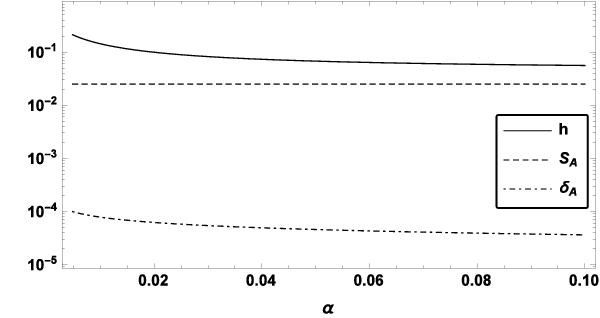
Notice that the ideal MHD solutions for the untwisted regions, i.e. inside ($0<r<a$) and outside ($r>R$) the flux tube, are valid in the jump conditions (34a) and (34b) only if the following condition is established (see Stenuit et al. 1998; Goossens et al. 2011)

$$\delta_{A}\leq S_{A}=\frac{R-a}{2},$$

(36)

where $\delta_{A}=\big|\frac{\omega}{|\Delta|}(\nu+\eta)\big|^{1/3}=(v_{A_{\rm i}}R)^{1/3}\big|\frac{\omega}{|\Delta|}(\frac{1}{\mathcal{R}_{v}}+\frac{1}{\mathcal{R}_{m}})\big|^{1/3}$ is a measure of the thickness of the resonance layer (see Sakurai et al. 1991a). Here $\nu=\frac{v_{A_{\rm i}}R}{\mathcal{R}_{v}}$, $\eta=\frac{v_{A_{\rm i}}R}{\mathcal{R}_{m}}$ and $\mathcal{R}_{v}$ are the kinematic viscosity, magnetic diffusivity and viscus Reynolds number, respectively. The classical values of viscus and resistive Reynolds numbers of the solar corona are about $10^{14}$ and $10^{13}$, respectively (see Colub & Pasachoff 1997). In Fig. 3, we also plot $\delta_{A}$ for the aforementioned values of the Reynolds and Lundquist numbers. Figure clears that the condition (36) is respected.

Substituting the ideal solutions (29) and (29) in the jump conditions (34a) and (34b) and eliminating $A_{\rm i}$ and $A_{\rm e}$, one can find the dispersion relation as

$$d_{0}(\tilde{\omega})+d_{1}(\tilde{\omega})=0,$$

(37)

where

$\displaystyle\begin{aligned} d_{0}(\tilde{\omega})=\frac{k_{z}}{\rho_{\rm e}(\tilde{\omega}^{2}-\omega_{A_{\rm e}}^{2})}\frac{K^{\prime}_{\rm m}(k_{z}R)}{K_{\rm m}(k_{z}R)}\\ ~~~~~~~~-\frac{k_{z}}{\rho_{\rm i}(\tilde{\omega}^{2}-\omega_{A_{\rm i}}^{2})}\frac{I^{\prime}_{\rm m}(k_{z}a)}{I_{\rm m}(k_{z}a)},\end{aligned}$

(38)

and

$\displaystyle\begin{aligned} &d_{1}(\tilde{\omega})=\\ &\frac{i\pi}{|\Delta|}\left[\frac{g_{B}}{\rho_{\rm i}B_{0}^{2}}-\frac{k_{z}}{\rho_{\rm e}(\tilde{\omega}^{2}-\omega_{A_{\rm e}}^{2})}\frac{2f_{B}B_{\varphi}}{\mu_{0}\rho_{\rm i}r_{\rm A}B_{0}}\frac{K^{\prime}_{\rm m}(k_{z}R)}{K_{\rm m}(k_{z}R)}\right]\\ &\times\left[g_{B}\frac{I_{m}(k_{z}r_{\rm A})}{I_{m}(k_{z}a)}-\frac{k_{z}}{\rho_{\rm i}(\tilde{\omega}^{2}-\omega_{A_{\rm i}}^{2})}\frac{2f_{B}B_{\varphi}B_{0}}{\mu_{0}r_{\rm A}}\frac{I^{\prime}_{\rm m}(k_{z}r_{\rm A})}{I_{\rm m}(k_{z}a)}\right].\end{aligned}$

(39)

Here $\tilde{\omega}=\omega-i\gamma$, in which $\omega$ and $\gamma$ are the mode frequency and the corresponding damping rate, respectively.

Using Eq. (2) in the last relation of Eq. (35) we get

$$\Delta=-\frac{B_{0}^{2}}{\mu_{0}\rho_{\rm i}}\frac{2m\alpha}{R(R-a)}\left(m\alpha\frac{r-a}{R(R-a)}+k\right),$$

(40)

which shows that in the limit of $a\rightarrow R$, i.e. when the twisted annulus region is removed, then $\Delta$ goes to infinity. As a result, in Eq. (39), $d_{1}=0$. In this case there is no resonant absorption and the dispersion relation (37) is the same as Eq. (25) in Bennett et al. (1999).

In the limit of thin tube approximation, using the first order asymptotic expansions for $I_{\rm m}(x)$ and $K_{\rm m}(y)$ one can get

$\displaystyle\begin{aligned} &\frac{I_{\rm m}(k_{z}r_{\rm A})}{I_{\rm m}(k_{z}a)}\simeq\left(\frac{r_{\rm A}}{a}\right)^{m},\\ &\frac{I^{\prime}_{\rm m}(k_{z}r_{\rm A})}{I_{\rm m}(k_{z}a)}\simeq\frac{m}{k_{z}r_{\rm A}}\left(\frac{r_{\rm A}}{a}\right)^{m},\\ &\frac{I^{\prime}_{\rm m}(k_{z}a)}{I_{\rm m}(k_{z}a)}\simeq\frac{m}{k_{z}a},\\ &\frac{K^{\prime}_{\rm m}(k_{z}R)}{K_{\rm m}(k_{z}R)}\simeq-\frac{m}{k_{z}R}.\end{aligned}$

(41)

Using the above approximations, the dispersion relation (37) reduces to

$\displaystyle\begin{aligned} &\frac{\rho_{\rm i}(\tilde{\omega}^{2}-\omega_{A_{\rm i}}^{2})}{R}+\frac{\rho_{\rm e}(\tilde{\omega}^{2}-\omega_{A_{\rm e}}^{2})}{a}\\ &~~~~~~~~-\frac{i\pi}{|\Delta|}\left(\frac{r_{\rm A}}{a}\right)^{m}\left(\frac{g_{\rm B}}{B_{0}^{2}}\rho_{\rm e}(\tilde{\omega}^{2}-\omega_{A_{\rm e}}^{2})+\frac{2mf_{B}B_{\varphi}}{\mu_{0}r_{\rm A}B_{0}R}\right)\\ &~~~~~~~~~~~~~~~~~\times\left(\frac{g_{\rm B}}{m}(\tilde{\omega}^{2}-\omega_{A_{\rm i}}^{2})-\frac{2f_{B}B_{\varphi}B_{0}}{\mu_{0}\rho_{\rm i}r_{\rm A}^{2}}\right)=0.\end{aligned}$

(42)

Notice that we look for the frequencies in the range of $\omega_{A_{\rm i}}<\omega<\omega_{A_{\rm e}}$, in which the resonant absorption occurs. Here $\omega_{A_{\rm i}}=k_{z}\frac{B_{\rm 0}}{\sqrt{\mu_{\rm 0}\rho_{\rm i}}}$ and $\omega_{A_{\rm e}}=k_{z}\frac{B_{\rm 0}}{\sqrt{\mu_{\rm 0}\rho_{\rm e}}}$ are the interior and exterior Alfvén frequencies, respectively. In the next section, we solve Eq. (42) analytically to obtain the frequency and damping rate of the kink MHD modes.

Here, we are interested in studying the effect of the twist parameter $\alpha$ on the frequencies, $\omega$, and the damping rates, $\gamma$, of the kink ($m=1$) MHD modes in a resonantly damped coronal loop. To this aim, we need to solve Eq. (42). First, we use the dimensionless quantities $\bar{r}=r/R$, $\bar{L}=L/R$, $\bar{B}=B/B_{0}$ and $\bar{\tilde{\omega}}=\tilde{\omega}/(v_{A_{\rm i}}/R)$. Thus, Eq. (42) can be recast in dimensionless form as

$\displaystyle\begin{aligned} &\zeta(\tilde{\omega}^{2}-\omega_{A_{\rm i}}^{2})+\frac{1}{q}(\tilde{\omega}^{2}-\omega_{A_{\rm e}}^{2})\\ &~~~~~~~~-\frac{i\pi}{|\Delta|}\left(\frac{r_{\rm A}}{a}\right)^{m}\left(g_{\rm B}(\tilde{\omega}^{2}-\omega_{A_{\rm e}}^{2})+\frac{2\zeta mf_{B}B_{\varphi}}{r_{\rm A}}\right)\\ &~~~~~~~~~~~~~~~~\times\left(\frac{g_{\rm B}}{m}(\tilde{\omega}^{2}-\omega_{A_{\rm i}}^{2})-\frac{2f_{B}B_{\varphi}}{r_{\rm A}^{2}}\right)=0,\end{aligned}$

(43)

where we have dropped the bars for simplicity. Here $q\equiv a/R$. Equation (43) yields a quadratic equation for $\tilde{\omega}^{2}$ as follows

$\displaystyle c_{1}\tilde{\omega}^{4}+c_{2}\tilde{\omega}^{2}+c_{3}=0,$

(44)

where

$\displaystyle\begin{aligned} &c_{1}=-\frac{i\pi}{|\Delta|}\left(\frac{r_{\rm A}}{q}\right)^{m}\frac{g_{B}^{2}}{m},\\ &c_{2}=\left(\zeta+\frac{1}{q}\right)+\frac{i\pi}{|\Delta|}\left(\frac{r_{\rm A}}{q}\right)^{m}\\ &\times\left[\frac{g_{B}^{2}}{m}\left(\omega_{A_{\rm i}}^{2}+\omega_{A_{\rm e}}^{2}\right)+\frac{2f_{B}g_{B}B_{\varphi}}{r_{\rm A}^{2}}\left(1-\zeta r_{\rm A}\right)\right],\\ &c_{3}=-\zeta\omega_{A_{\rm i}}^{2}\left(1+\frac{1}{q}\right)-\frac{i\pi}{|\Delta|}\left(\frac{r_{\rm A}}{q}\right)^{m}\zeta\\ &\times\left[\frac{g_{B}^{2}}{m}\omega_{A_{\rm i}}^{4}-\frac{4mf_{B}^{2}B_{\varphi}^{2}}{r_{\rm A}^{3}}+\frac{2f_{B}g_{B}B_{\varphi}\omega_{A_{\rm i}}^{2}}{r_{\rm A}^{2}}(1-r_{\rm A})\right].\end{aligned}$

(45)

It is straightforward to find the solutions of Eq. (44), $\tilde{\omega}=\omega-i\gamma$, as follows

$\displaystyle\begin{aligned} &\omega_{\pm}=\frac{1}{\sqrt{\mathfrak{R}_{\pm}^{2}+\mathfrak{I}_{\pm}^{2}}}\left(\sqrt{\mathfrak{\chi_{\pm}}^{2}+\Theta_{\pm}^{2}}+\mathfrak{\chi_{\pm}}\right)^{1/2},\\ &\gamma_{\pm}=\frac{1}{\sqrt{\mathfrak{R}_{\pm}^{2}+\mathfrak{I}_{\pm}^{2}}}\left(\sqrt{\mathfrak{\chi_{\pm}}^{2}+\Theta_{\pm}^{2}}-\mathfrak{\chi_{\pm}}\right)^{1/2},\end{aligned}$

(46)

where

$\displaystyle\begin{aligned} &\chi_{\pm}=c_{3_{\rm R}}\mathfrak{R}_{\pm}+c_{3_{\rm I}}\mathfrak{I}_{\pm},\\ &\Theta_{\pm}=c_{3_{\rm I}}\mathfrak{R}_{\pm}-c_{3_{\rm R}}\mathfrak{I}_{\pm},\\ &\mathfrak{R_{\pm}}=-c_{2_{\rm R}}\pm\left(\frac{\sqrt{c_{\rm 4}^{2}+c_{\rm 5}^{2}}+c_{\rm 4}}{2}\right)^{1/2},\\ &\mathfrak{I_{\pm}}=-c_{2_{\rm I}}\pm\left(\frac{\sqrt{c_{\rm 4}^{2}+c_{\rm 5}^{2}}-c_{\rm 4}}{2}\right)^{1/2},\end{aligned}$

(47)

with

$\displaystyle\begin{aligned} &c_{4}=c_{2_{\rm R}}^{2}-c_{2_{\rm I}}^{2}+4c_{1_{\rm I}}c_{3_{\rm I}},\\ &c_{5}=2c_{2_{\rm R}}c_{2_{\rm I}}-4c_{1_{\rm I}}c_{3_{\rm R}}.\end{aligned}$

(48)

Here, the subscripts $R$ and $I$ denote the real and imaginary parts of a given complex quantity.

For a typical coronal loop, we take $L=10^{5}$ km, $R/L=0.005,0.01$, $\zeta=\rho_{\rm i}/\rho_{\rm e}=2,4$, $\rho_{\rm i}=2\times 10^{-14}$ g $\rm{cm^{-3}}$ and $B_{0}=100$ G. So, one finds $v_{A_{\rm i}}=B_{0}/\sqrt{\mu_{0}\rho_{\rm i}}=2000$ km $\rm{s^{-1}}$ in this loop. We assume that the magnetic twist takes place in a thin layer of thickness $R-a=0.05R$. So we have $q=0.95$. In the thin boundary approximation, we can set the location of the resonance point at the tube surface, i.e. $r_{\rm A}\simeq R$.

Using Eq. (46) we obtain two roots of $\omega_{\pm}$ which their values take place in the range of $\omega_{A_{\rm i}}<\omega_{-}<\omega_{A_{\rm e}}$ and $\omega_{+}>\omega_{A_{\rm e}}$. Therefore, $\omega_{-}$ is our physical root and $\omega_{+}$ should be ruled out, because it does not give rise to the resonant absorption. As we have already mentioned, in the limit of $q\rightarrow 1$ (i.e. $a\rightarrow R$), we have $\Delta\rightarrow\infty$. In this case, from Eq. (45) we obtain $c_{1}=c_{2_{\rm I}}=c_{3_{\rm I}}=0$. Hence, in the absence of twisted annulus region, form Eqs. (46)-(48) we get

$\displaystyle\begin{aligned} &\omega_{-}=\sqrt{\frac{2\zeta}{\zeta+1}}~\omega_{A_{\rm i}}=\omega_{\rm kink},\\ &\gamma_{-}=0,\end{aligned}$

(49)

where $\omega_{\rm kink}$ is the kink mode frequency of an untwisted loop in the thin tube approximation (see e.g. Goossens et al. 2009).

Here, we are interested to obtain a minimum value for the twist parameter $\alpha=\alpha_{\rm min}$ which is required to excite the resonance. The exact value of $\alpha_{\rm min}$ is determined as the root of the following equation

$\displaystyle\omega_{-}|_{\alpha=\alpha_{\rm min}}=\omega_{A}(R)|_{\alpha=\alpha_{\rm min}}.$

(50)

We solve this numerically and conclude that the result obtained for $\alpha_{\rm min}$ satisfies the following relation

$\displaystyle\omega_{-}|_{\alpha=\alpha_{\rm min}}\simeq\omega_{\rm kink}.$

(51)

Equating right hand sides of Eqs. (50) and (51), one can get an approximate expression for $\alpha_{\rm min}$ as

$\displaystyle\alpha_{\rm min}\simeq\pi\left(\frac{R}{L}\right)\left(\frac{l}{m}\right)\left(\sqrt{\frac{2\zeta}{\zeta+1}}-1\right).$

(52)

For instance, taking $\zeta=2$ and $R/L=0.01$, for the fundamental ($l=1$), first overtone ($l=2$) and second overtone ($l=3$) kink ($m=1$) modes, Eq. (52) gives $\alpha_{\min}=$0.0049, 0.0097 and 0.0146, respectively. The relative error of the results of Eq. (52) with respect to the exact solutions of Eq. (50) is about $0.6\%$.

Figures 4, 5, and 6 illustrate the frequencies ($\omega_{-}=\omega_{ml}$), the damping rates ($\gamma_{-}=\gamma_{ml}$) and the ratio of the frequency to the damping rate $(\omega_{ml}/\gamma_{ml})$ of the fundamental ($l=1$) and first/second overtone $(l=2,3)$ kink ($m=1$) modes versus the twist parameter $\alpha$, respectively. Figures show that (i) the frequencies and damping rates increase when the twist parameter increases. (ii) The ratio of the oscillation frequency to the damping rate $\omega/\gamma$ decreases when the twist parameter increases. The result, interestingly enough, is that for the fundamental ($l=1$) kind ($m=1$) mode, for the twist parameter $\alpha=0.0147$ we obtain $\omega_{11}/(2\pi\gamma_{11})=3$ which is in good agreement with the observations reported by Nakariakov et al. (1999), Wang & Solanki (2004), and Verwichte et al. (2004). Here, the behaviour of $\omega$ and $\gamma$ versus the twist parameter $\alpha$ are the same as that obtained by Karami & Bahari (2010) but for the resonant absorption due to the radial density structuring. (iii) For a given $\alpha$ and $\zeta$, when $R/L$ increases then $\omega$ increases, $\gamma$ decreases and $\omega/\gamma$ increases. (iv) For a given $\alpha$ and $R/L$, when $\zeta$ increases, the frequency and the ratio $\omega/\gamma$ increase. However, this behavior for the damping rate holds only for large values of the twist parameter. Moreover, increasing $\zeta$ does not affect the ratio $\omega/\gamma$ for large values of $\alpha$. (v) Note that based on Eq. (52), $\alpha_{\rm min}$ is a function of $m$, $l$, $\zeta$ and $R/L$. Therefore, for each set of these parameters, the start points of the diagrams in Figs. 4 to 6 have different $\alpha_{\rm min}$ values. Also to avoid the kink instability in our model, following Hood & Priest (1979) we consider the twist value $\phi_{\rm twist}\lesssim\phi_{c\rm}=3.3\pi$ and consequently obtain an upper limit for the twist parameter as $\alpha_{\rm max}=(R/L)\phi_{\rm c}$. Hence, the diagrams in Figs. 4 to 6 with different $R/L$ have different $\alpha_{\rm max}$ cut-offs.

Figure 7 presents variations of $\omega$, $\gamma$ and $\omega/\gamma$ for the fundamental ($l=1$) kink ($m=1$) mode versus the thickness of the twisted layer, $d\equiv R-a$. Figure shows that when $d$ increases both frequency and damping rate increase but the ratio of the frequency to the damping rate decreases. This behaviour holds also for the first and second overtone ($l=2,3$) kink modes. Figure 7 clarifies that in the limit of $d\rightarrow 0$ (i.e. $a\rightarrow R$), we have $\omega_{11}\rightarrow\omega_{\rm kink}=\sqrt{\frac{2\zeta}{\zeta+1}}~\omega_{A_{\rm i}}\simeq 0.03628$ (in units of 2 rad s^-1) and $\gamma_{11}\rightarrow 0$. Note that the result of $\omega/\gamma$ for the fundamental mode of kink oscillations is in good agreement with that obtained for the resonant absorbtion due to the radial density structuring (see e.g. Ruderman & Roberts 2002; Ruderman & Terradas 2013).

In Fig. 8, the period ratios of the fundamental to the first overtone, $P_{1}/P_{2}$, and to the second overtone, $P_{1}/P_{3}$, of the kink ($m=1$) modes are plotted versus the twist parameter $\alpha$. Figure shows that (i) when the twist parameter increases, the values of $P_{1}/P_{2}$ and $P_{1}/P_{3}$ decrease from their canonical values, 2 and 3, respectively. (ii) The density ratio $\zeta=\rho_{\rm i}/\rho_{\rm e}$ does not affect the period ratio. Notice that the solid curve overlaps the dashed one. (iii) For a given $\alpha$ and $\zeta$, the period ratio decreases when $R/L$ decreases. In Fig. 9, we plot variations of the period ratios $P_{1}/P_{2}$ and $P_{1}/P_{3}$ versus the thickness of the twisted layer $d$. Figure 9 shows that the period ratios decrease with increasing $d$.

Note that the deviations of the period ratios $P_{1}/P_{2}$ and $P_{1}/P_{3}$ from their canonical values provide useful information about the magnetic twist structuring within the loop. For instance, the observed value $P_{1}/P_{2}=1.795$ reported by Van Doorsselaere et al. (2007) can be justified with the twist parameter $\alpha=0.0718$. Van Doorsselaere et al. (2007) also reported the identification of the second overtone of the kink mode by re-analyzing the transverse oscillations of coronal loops observed by TRACE on 13 May 2001. The period ratio of fundamental to second overtone kink mode found to be $P_{1}/P_{3}=2.89$ which can be justified with the twist parameter $\alpha=0.0460$. Table 1 summarizes the twist parameters and the corresponding twist values, $\phi_{\rm twist}=\big(\frac{L}{R}\big)\alpha$, predicted by our model in order to justify some observed period ratios $P_{1}/P_{2}$ and $P_{1}/P_{3}$ of the kink ($m=1$) modes. Note that the magnetic twist values $\phi_{\rm twist}$ predicted by our model are in the range of the observational values reported by Kwon & Chae (2008) and Wang et al. (2015).

Here, we investigated the resonant absorption of kink MHD modes by magnetic twist in coronal loops. To this aim, we considered a thin straight cylindrical flux tube with a twisted magnetic field in a thin layer at the boundary of the loop and a straight magnetic field everywhere else. The magnetic twist causes a radial Alfvén frequency gradient and consequently gives rise to the resonant absorption. We assumed the plasma density to be constant but different in the interior and exterior regions of the loop. We obtained the solutions of ideal MHD equations for the interior and exterior regions of the tube. Then, we investigated a number of possible instabilities that may arise in our model and concluded that these instabilities can be avoided in the present model. We also derived the dispersion relation by using the appropriate connection formula introduced by Sakurai et al. (1991a). In thin tube thin boundary approximation, we solved analytically the dispersion relation and obtained the frequencies and damping rates of the fundamental $(l=1)$ and first/second overtone $(l=2,3)$ kink $(m=1)$ modes. Our results show the following.

• •

  The frequencies and damping rates increase when the twist parameter increases.

• •

  The ratio of the fundamental frequency to its corresponding damping rate of the kink ($m=1$) modes can well justify the rapid damping of kink MHD waves ($\omega/(2\pi\gamma)\simeq 3$) reported by the observations. This confirms the high efficiency of resonant absorbtion due to the magnetic twist.

• •

  For a given twist parameter $\alpha$ and density ratio $\zeta=\rho_{\rm i}/\rho_{\rm e}$ by increasing $R/L$, the frequencies increase, the damping rates decrease and the ratio of the frequency to the damping rate increases.

• •

  By increasing the thickness of the twisted layer, the frequency and the damping rate increase but the ratio of the frequency to the damping rate and the period ratio decrease.

• •

  For a given $\alpha$ and $\zeta$, the period ratio decreases with decreasing $R/L$. Furthermore, the density ratio $\zeta$ does not affect the period ratio.

• •

  The period ratios $P_{1}/P_{2}$ and $P_{1}/P_{3}$ with increasing the twist parameter, decrease from 2 and 3, respectively. For some special values of the twist parameter, the values of $P_{1}/P_{2}$ and $P_{1}/P_{3}$ predicted by our model can justify the observations.

The authors thank the anonymous referee for very valuable comments. The authors also thank Anna Tenerani, Michael Ruderman, Robert Erdélyi and Markus Aschwanden for useful discussions.

References

- [1] Andries J., Goossens M., Hollweg J. V., Arregui I., Van Doorsselaere T., 2005, A&A, 430, 1109
- [2] Andries J., Van Doorsselaere T., Roberts B., Verth G., Verwichte E., Erdélyi R., 2009, Space Sci. Rev., 149, 3
- [3] Antolin P., Okamoto T. J., De Pontieu B., Uitenbroek H., Van Doorsselaere T., Yokoyama T., 2015, ApJ, 809, 72
- [4] Arregui I., Soler R., Ballester J. L., Wright A. N., 2011, A&A, 533, A60
- [5] Aschwanden M. J., Fletcher L., Schrijver C. J., Alexander D., 1999, ApJ, 520, 880
- [6] Aschwanden M. J., 2005, Physics of the Solar Corona. Springer, Berlin
- [7] Ballai I., Jess D. B., Douglas M., 2011, A&A, 534, A13
- [8] Baty H., Heyvaerts J., 1996, A&A, 308, 935
- [9] Bennett K., Roberts B., Narain U., 1999, Sol. Phys., 185, 41
- [10] Biskamp D., 2000, Magnetic Reconnection in Plasmas. Cambridge Univ. Press, Cambridge
- [11] Carter B. K., Erdélyi R., 2007, A&A, 475, 323
- [12] Carter B. K., Erdélyi R., 2008, A&A, 481, 239
- [13] Chae J., Wang H., Qiu J., Goode P. R., Wilhelm K., 2000, ApJ, 533, 535
- [14] Chae J., Moon Y. J., 2005, ApJ, 629, 1110
- [15] Colub L., Pasachoff J. M., 1997, The Solar Corona. Cambridge Univ. Press, Cambridge
- [16] De Moortel I., 2005, Phil. Trans. R. Soc. A, 363, 2743
- [17] De Moortel I., Nakariakov V. M., 2012, Phil. Trans. R. Soc. A, 370, 3193
- [18] Davila J. M., 1987, ApJ, 317, 514
- [19] Erdélyi R., Goossens M., 1995, A&A, 294, 575
- [20] Erdélyi R., Goossens M., 1996, A&A, 313, 664
- [21] Erdélyi R., Carter B. K., 2006, A&A, 455, 361
- [22] Erdélyi R., Fedun V., 2006, Sol. Phys., 238, 41
- [23] Erdélyi R., Fedun V., 2007, Sol. Phys., 246, 101
- [24] Erdélyi R., Fedun V., 2010, Sol. Phys., 263, 63
- [25] Furth H. P., Killeen J., Rosenbluth M. N., 1963, Phys. Fluids, 6, 459
- [26] Furth H. P., Rutherford P. H., Selberg H., 1973, Phys. Fluids, 16, 1054
- [27] Goldstone R. J., Rutherford P. H., 1995, Introduction to plasma physics. IOP Publishing, London
- [28] Goossens M., Hollweg J. V., Sakurai T., 1992, Sol. Phys., 138, 233
- [29] Goossens M., Andries J., Aschwanden M. J., 2002, A&A, 394, L39
- [30] Goossens M., Terradas J., Andries J., Arregui I., Ballester J. L., 2009, A&A, 503, 213
- [31] Goossens M., Erdélyi R., Ruderman M. S., 2011, Space Sci. Rev., 158, 289
- [32] Heyvaerts J., Priest E. R., 1983, A&A, 117, 220
- [33] Hood A. W., Priest E. R., 1979, Sol. Phys., 64, 303
- [34] Hood A. W., Cargill P. J., Browning P. K., Tam K. V., 2016, ApJ, 817, 5
- [35] Ionson J. A., 1978, ApJ, 226, 650
- [36] Karami K., Barin M., 2009, MNRAS, 394, 521
- [37] Karami K., Nasiri S., Amiri S., 2009, MNRAS, 394, 1973
- [38] Karami K., Bahari K., 2010, Sol. Phys., 263, 87
- [39] Karami K., Bahari K., 2012, ApJ, 757, 186
- [40] Kruskal M. D., Johnson J. L., Gottlieb M. B., Goldman L. M., 1958, Phys. Fluids, 1, 421
- [41] Kwon R. Y., Chae J., 2008, ApJ, 677, L141
- [42] Magara T., Shibata K., 1999, ApJ, 514, 456
- [43] Mikić Z., Schnack D. D., VanHoven G., 1990, ApJ, 361, 690
- [44] Nakariakov V. M., Ofman L., DeLuca E. E., Roberts B., Davila J. M., 1999, Science, 285, 862
- [45] Nakariakov V. M., Ofman L., 2001, A&A, 372, L53
- [46] Priest E. R., 2014, Magnetohydrodynamics of the Sun. Cambridge Univ. Press, Cambridge
- [47] Roberts B., Edwin P. M., Benz A. O., 1984, ApJ, 279, 857
- [48] Ruderman M. S., Roberts B., 2002, ApJ, 577, 475
- [49] Ruderman M. S., 2007, Sol. Phys., 246, 119
- [50] Ruderman M. S., Erdélyi R., 2009, Space Sci. Rev., 149, 199
- [51] Ruderman M. S., 2011, A&A, 534, A78
- [52] Ruderman M. S., 2015, A&A, 575, A130
- [53] Ruderman M. S., Terradas J., 2013, A&A, 555, A27
- [54] Sakurai T., Goossens M., Hollweg J. V., 1991a, Sol. Phys., 133, 227
- [55] Sakurai T., Goossens M., Hollweg J. V., 1991b, Sol. Phys., 133, 247
- [56] Sewel G., 2005, The Nummerical Solution of Ordinary and Partial Differential Equations. 2nd edn., John Wiley & Sons, New Jersey
- [57] Shafranov V. D., 1957, J. Nucl. Energy II, 5, 86
- [58] Soler R., Terradas J., Oliver R., Ballester J. L., Goossens M., 2010, ApJ, 712, 875
- [59] Soler R., Terradas J., 2015, ApJ, 803, 43
- [60] Steinolfson R. S., Davila J. M., 1993, ApJ, 415, 354
- [61] Stenuit H., Keppens R., Goossens M., 1998, A&A, 331, 392
- [62] Tenerani A., Rappazzo A. F., Velli M., Pucci F., 2015, ApJ, 801, 145
- [63] Terradas J., Oliver R., Ballester J. L., 2006a, ApJ, 642, 533
- [64] Terradas J., Oliver R., Ballester J. L., 2006b, ApJ, 650, L91
- [65] Terradas J., Andries J., Goossens M., Arregui I., Oliver R., Ballester J. L., 2008, ApJ, 687, L115
- [66] Terradas J., Goossens M., 2012, A&A, 548, A112
- [67] van der Holst B., Beliën A. J. C., Goedbloed J. P., Nool M., van der Ploeg A., 1999, Phys. Plasmas, 6, 1554
- [68] Van Doorsselaere T., Andries J., Poedts S., Goossens M., 2004, ApJ, 606, 1223
- [69] Van Doorsselaere T., Nakariakov V. M., Verwichte E., 2007, A&A, 473, 959
- [70] Van Doorsselaere T., Birtill D. C. C., Evans G. R., 2009, A&A, 508, 1485
- [71] Verth G., Terradas J., Goossens M., 2010, ApJL, 718, L102
- [72] Verwichte E., Nakariakov V. M., Ofman L., Deluca E. E., 2004, Sol. Phys., 223, 77
- [73] Wang T. J., Solanki S. K., 2004, A&A, 421, L33
- [74] Wang H., Cao W., Liu C., Xu Y., Liu R., Zeng Z., Chae J., Ji H., 2015, Nature Communications, 6, 70086
- [75] Wesson J., 2004, Tokamaks. Oxford Univ. Press, Oxford