跳到论文正文
W Papers独立论文阅读器 arXiv:1507.02542 论文正文 计算阅读时间 · 0%
引用这篇论文根据当前论文元数据生成,正式投稿前建议核对。


License: arXiv.org perpetual non-exclusive license
arXiv:1507.02542v1 [math.AP] 09 Jul 2015

A piezoelectric Euler-Bernoulli beam with dynamic boundary control: stability and dissipative FEMThanks: The authors were supported by the doctoral school PDE-Tech of TU Wien and the FWF-project I395-N16. The authors acknowledge a sponsorship by Clear Sky Ventures. We are grateful to A. Kugi and T. Meurer for introducing us to this topic, their help, and the many stimulating discussions.

Maja Miletic Address: Institute for Analysis and Scientific Computing, Technical University Vienna, Wiedner Hauptstr. 8, A-1040 Vienna, AUSTRIA Email address: mmiletic@asc.tuwien.ac.at, anton.arnold@tuwien.ac.at and Anton Arnold
Abstract.

We present a mathematical and numerical analysis on a control model for the time evolution of a multi-layered piezoelectric cantilever with tip mass and moment of inertia, as developed by Kugi and Thull [31]. This closed-loop control system consists of the inhomogeneous Euler-Bernoulli beam equation coupled to an ODE system that is designed to track both the position and angle of the tip mass for a given reference trajectory. This dynamic controller only employs first order spatial derivatives, in order to make the system technically realizable with piezoelectric sensors. From the literature it is known that it is asymptotically stable [31]. But in a refined analysis we first prove that this system is not exponentially stable.

In the second part of this paper, we construct a dissipative finite element method, based on piecewise cubic Hermitian shape functions and a Crank-Nicolson time discretization. For both the spatial semi-discretization and the full x−tx-t–discretization we prove that the numerical method is structure preserving, i.e. it dissipates energy, analogous to the continuous case. Finally, we derive error bounds for both cases and illustrate the predicted convergence rates in a simulation example.

Key words and phrases: 
beam equation and boundary feedback control and asymptotic stability and dissipative Galerkin method and error estimates
2010 Mathematics Subject Classification
Primary 35B35, 65M60 ; Secondary 35P20, 74S05, 93D15

1. Model

The Euler-Bernoulli beam (EBB) equation with tip mass is a well-established model with a wide range of applications: for oscillations in telecommunication antennas, or satellites with flexible appendages [2, 5], flexible wings of micro air vehicles [8], and even vibrations of tall buildings due to external forces [41]. The interest of engineers and mathematicians in the corresponding control problems started in the 1980s. So various boundary control laws have been devised and mathematically analyzed in the literature – with the stabilization of the system being a key objective (cf. [34]). Soon afterwards, also exponentially stable controllers were developed which require, however, higher order boundary controls for an EBB with both applied tip mass and moment of inertia [42]. On the other hand, if only a tip mass is applied, lower order controls are sufficient for exponential stabilization [12]. In spite of this progress, and due to its widespread technological applications, considerable research on EBB-control problems is still underway: In the more recent papers [22, 20] exponential stability of related control systems was established by verifying the Riesz basis property. For the exponential stability of a more general class of boundary control systems (including the Timoshenko beam) in the port-Hamiltonian approach we refer to [49].

We shall analyze an inhomogeneous multi-layered piezoelectric EBB with applied tip mass and moment of inertia, coupled to a dynamic controller that uses only low order boundary measurements. This system was introduced by Kugi and Thull in [31] to independently control the tip position and the tip angle of a piezoelectric cantilever along prescribed trajectories. This beam is composed of piezoelectric layers and the electrode shape of the layers was used as an additional degree of freedom in the controller design. The sensor layers were given rectangular and triangular shaped electrodes, so that the charge measured is proportional to the tip deflection and the tip angle, respectively. The actuator layers were also assumed to be covered with rectangular and triangular shaped electrodes, with the following motivation: A voltage supplied to an actuator with rectangular (or triangular) shaped electrodes acts in the same way on the structure as a bending moment (or force) at the tip of the beam. The key issue of [31] was to devise a stable feedback control model for that beam, such that it evolves asymptotically (as t→∞t\to\infty) as a prescribed reference trajectory. More precisely, that controller allows to track the position and the angle of the tip mass at the same time. To solve the trajectory planning task, the concept of differential flatness (cf. [3]) was employed. Thereby, the control inputs and the beam bending deflection were parametrized by the flat outputs and their time derivatives. The boundary controller constructed there has a dynamic design, thus coupling the governing PDEs of the beam with a system of ODEs in the feedback part. In order to render the system experimentally and technically realizable, it is crucial that the controller only involves boundary measurements up to the first spatial derivative – at the (small) price of loosing exponential stability (as we shall see here below).

The goal of the present paper is first to complete the analysis of [31], proving that this hybrid system is asymptotically stable but not exponentially stable. This part is an extension of Rao’s analysis [42] to dynamic controllers and inhomogeneous beams. In our second, and in fact main part we shall develop and analyze a dissipative finite element method (FEM) for the control system.

Now we specify the problem under consideration, an inhomogeneous EBB of length LL, clamped at the left end x=0x=0, and with tip mass, moment of inertia, and boundary control at x=Lx=L. In the following linear system (1.1)–(1.5), we actually consider the evolution of the trajectory error system. So, u⁡(t,x)u(t,x) denotes the deviation of the actual beam deflection from the desired reference trajectory. Similarly, Θ1,2​(t)\Theta_{1,2}(t) denote the difference between the applied voltages to the electrodes of the piezoelectric layers and the ones specified by the feedforward controller.

(1.1) μ⁡(x)​ut​t+(Λ⁡(x)​ux​x)x​x\displaystyle\mu(x)u_{tt}+(\Lambda(x)u_{xx})_{xx} =\displaystyle= 0,0<x⁡<L,t>​0,\displaystyle 0,\quad 0<x<L,\,t>0,
(1.2) u⁡(t,0)\displaystyle u(t,0) =\displaystyle= 0,t>0,\displaystyle 0,\quad t>0,
(1.3) ux​(t,0)\displaystyle u_{x}(t,0) =\displaystyle= 0,t>0,\displaystyle 0,\quad t>0,
(1.4) J​ux​t​t​(t,L)+(Λ​ux​x)​(t,L)+Θ1​(t)\displaystyle Ju_{xtt}(t,L)+(\Lambda u_{xx})(t,L)+\Theta_{1}(t) =\displaystyle= 0,t>0,\displaystyle 0,\quad t>0,
(1.5) M​ut​t​(t,L)−(Λ​ux​x)x​(t,L)+Θ2​(t)\displaystyle Mu_{tt}(t,L)-(\Lambda u_{xx})_{x}(t,L)+\Theta_{2}(t) =\displaystyle= 0,t>0.\displaystyle 0,\quad t>0.

Here, μ∈C4​[0,L]\mu\in C^{4}[0,L] denotes the linear mass density of the beam and Λ∈C4​[0,L]\Lambda\in C^{4}[0,L] is the flexural rigidity of the beam. Both functions are assumed to be strictly positive and bounded. MM and JJ denote, respectively, the mass and the moment of inertia of the rigid body attached at x=Lx=L. Equation (1.4) states that the beam bending moment at x=Lx=L (i.e. Λ⁡(L)​ux​x​(t,L)\Lambda(L)u_{xx}(t,L)) plus the bending moment of the tip body (i.e. J​ux​t​t​(t,L)Ju_{xtt}(t,L)) is balanced by the control input −Θ1-\Theta_{1}. Similarly, (1.5) describes that the total force at the free end, equal to shear force at the tip (i.e. −(Λ​ux​x)x​(t,L)-(\Lambda u_{xx})_{x}(t,L)) plus the tip mass force M​ut​tMu_{tt}, cancels with the control input Θ2\Theta_{2}.

The proposed control law has the goal to drive the error system to the zero state as t→∞t\to\infty. It reads:

(1.6) (ζ1)t​(t)=A1​ζ1​(t)+b1​ux​t​(t,L),(ζ2)t​(t)=A2​ζ2​(t)+b2​ut​(t,L),Θ1​(t)=k1​ux​(t,L)+c1⋅ζ1​(t)+d1​ux​t​(t,L),Θ2​(t)=k2​u​(t,L)+c2⋅ζ2​(t)+d2​ut​(t,L),\begin{array}[]{rcl}(\zeta_{1})_{t}(t)&=&A_{1}\zeta_{1}(t)+b_{1}u_{xt}(t,L),\\ (\zeta_{2})_{t}(t)&=&A_{2}\zeta_{2}(t)+b_{2}u_{t}(t,L),\\ \Theta_{1}(t)&=&k_{1}u_{x}(t,L)+c_{1}\cdot\zeta_{1}(t)+d_{1}u_{xt}(t,L),\\ \Theta_{2}(t)&=&k_{2}u(t,L)+c_{2}\cdot\zeta_{2}(t)+d_{2}u_{t}(t,L),\end{array}

with the auxiliary variables ζ1,ζ2∈C⁡([0,∞),ℝn)\zeta_{1},\zeta_{2}\in C([0,\infty);\mathbb{R}^{n}) and Θ1,Θ2∈C[0,∞)\Theta_{1},\Theta_{2}\in C[0,\infty). Moreover, A1,A2∈ℝn×nA_{1},A_{2}\in\mathbb{R}^{n\times n} are Hurwitz11 1 A square matrix is called a Hurwitz matrix if all its eigenvalues have negative real parts. matrices, b1,b2,c1,c2∈ℝnb_{1},b_{2},c_{1},c_{2}\in\mathbb{R}^{n} vectors and k1,k2,d1,d2∈ℝk_{1},k_{2},d_{1},d_{2}\in\mathbb{R}. We assume that the coefficients k1k_{1} and k2k_{2} are positive and that the transfer functions 𝒢j(s)=(sI−Aj)−1bj⋅cj+dj,j=1,2\mathcal{G}_{j}(s)=(sI-A_{j})^{-1}b_{j}\cdot c_{j}+d_{j},\,j=1,2 satisfy

R​e​(𝒢j​(i​ω))≥dj≥δj>0∀ω≥0,j=1,2Re({\mathcal{G}}_{j}(i\omega))\geq d_{j}\geq\delta_{j}>0\quad\forall\omega\geq 0,\;j=1,2

for some constants δ1\delta_{1} and δ2\delta_{2}. These assumptions imply that the transfer function is strictly positive real, or shortly SPR (for its definition we refer to [24], [35]). Then, it follows from the Kalman-Yakubovic-Popov Lemma (see [24], [35]) that there exist symmetric positive definite matrices PjP_{j}, positive scalars ϵj\epsilon_{j}, and vectors qj∈ℝnq_{j}\in\mathbb{R}^{n} such that

(1.7) Pj​Aj+Aj⊤​Pj\displaystyle P_{j}A_{j}+A_{j}^{\top}P_{j} =−qj​qj⊤−ϵj​Pj,\displaystyle=-q_{j}q_{j}^{\top}-\epsilon_{j}P_{j},
Pj​bj\displaystyle P_{j}b_{j} =cj−qj​2​(dj−δj),\displaystyle=c_{j}-q_{j}\sqrt{2(d_{j}-\delta_{j})},

for j=1,2.j=1,2. A SPR controller is defined as a controller with SPR transfer function. One motivation for this controller design is the fact that, in the finite dimensional case, the feedback interconnection of a passive system with a SPR controller yields a stable closed-loop system. This principle of passivity based controller design was generalized to the trajectory error dynamics of the multi-layered piezoelectric cantilever in [31].

(1.1)–(1.6) constitute a coupled PDE–ODE system for the beam deflection u⁡(x,t)u(x,t), the position of its tip u⁡(t,L)u(t,L), and its slope ux​(t,L)u_{x}(t,L), as well as the two control variables ζ1​(t)\zeta_{1}(t), ζ2​(t)\zeta_{2}(t). The main mathematical difficulty of this system stems from the high order boundary conditions (involving both xx- and tt- derivatives) which makes the analytical and numerical treatment far from obvious. Well-posedness of this system and asymptotic stability of the zero state were established in [31] using semigroup theory on an equivalent first order system (in time), a carefully designed Lyapunov functional, and LaSalle’s invariance principle.

In §2 we shall prove that this unique steady state is not exponentially stable. Let us compare this result to a similar system studied in [39] and §5.3 of [35], which also consists of an EBB coupled to a passivity based dynamic boundary control, but without the tip mass. Then, that system is exponentially stable.

As an introduction for our dissipative finite element method (FEM) in §3, we shall now briefly review several numerical strategies for the EBB from the literature. In [48] the authors propose a conditionally stable, central difference method for both the space and time discretization of the EBB equation. Their system models a beam, which has a tip mass with moment of inertia on the free end. At the fixed end a boundary control is applied in form of a control torque. Due to higher order boundary conditions, fictitious nodes are needed at both boundaries. In [15] the authors consider a damped, translationally cantilevered EBB, with one end clamped into a moving base (as a boundary control) and a tip mass with moment of inertia placed at the other. For their numerical treatment they considered a finite number of modes, thus obtaining an ODE system. In [32] the EBB with one free end (without tip mass, but with boundary torque control) was solved in the frequency domain: After Laplace transformation in time, the resulting ODEs could be solved explicitly.

The more elaborate approaches are based on FEMs: In [6] two space-time spectral element methods are employed to solve a simply supported, nonlinear, modified EBB subjected to forced lateral vibrations but with no mass attached: There, Hermitian polynomials, both in space and time, lead to strict stability limitations. But a mixed discontinuous Galerkin formulation with Hermitian cubic polynomials in space and Lagrangian spectral polynomials in time yields an unconditionally stable scheme. In [13] the authors present a semi-discrete (using cubic splines) and fully discrete Galerkin scheme (based on the Crank-Nicolson method) for the strongly damped, extensible beam equation with both ends hinged. [4] considers a EBB with tip mass at the free end, yielding a conservative hyperbolic system. The authors analyze a cubic B-spline based Galerkin method (including convergence analysis of the spatial semi-discretization) and put special emphasis on the subsequent parameter identification problem.

All these FEMs are for models without boundary control. Hence, we shall develop here a novel FEM for the mixed boundary control problem (1.1)-(1.6). There, the damping only appears due to the boundary control. Hence, our main focus will be on preserving the correct large-time behavior (i.e. dissipativity) in the numerical scheme. Our FEM is based on the second order (in time) EBB equation (1.1) and special care is taken for the boundary coupling to the ODE. In time we shall use a Crank-Nicolson discretization, which was also the appropriate approach for the decay of discretized parabolic equations in [1]. We remark that the modeling and discretization of boundary control systems as port-Hamiltonian systems also has this flavor of preserving the structure: For a general methodology on this spatial semi-discretization (leading to mixed finite elements) and its application to the telegrapher’s equations we refer to [18].

The paper is organized as follows: In §2 we first review the analytic setting from [31] for the EBB with boundary control. While this closed-loop system is asymptotically stable, we prove that it is not exponentially stable. Towards this analysis we derive the asymptotic behavior of the eigenvalues and eigenfunctions of the coupled system. In §3 we first discuss the weak formulation of our control system. Then we develop an unconditionally stable FEM (along with a Crank-Nicolson scheme in time), which dissipates an appropriate energy functional independently of the chosen FEM basis. We shall also derive error estimates (second order in space and time) of our scheme. In the numerical simulations of §4 we illustrate the proposed method and verify its order of convergence w.r.t. hh and Δ​t\Delta t.

2. Non-exponential decay

First we recall from [31] the analytical setting for (1.1)–(1.6) in the framework of semigroup theory. To cope with the higher order boundary conditions (1.4), (1.5) and the boundary terms on the r.h.s. of (1.6), the terms ut​(t,L)u_{t}(t,L), ux​t​(t,L)u_{xt}(t,L) were introduced as separate variables (following the spirit in earlier works [34, 20]). More precisely, ψ=M​v​(L)\psi=Mv(L) is the vertical momentum of the tip mass and ξ=J​vx​(L)\xi=Jv_{x}(L) its angular momentum, where v=utv=u_{t} is the velocity of the beam. Hence, we define the Hilbert space

ℋ:={z=(u,v,ζ1,ζ2,ξ,ψ)⊤:u∈H~02(0,L),v∈L2(0,L),ζ1,ζ2∈ℝn,ξ,ψ∈ℝ},\mathcal{H}:=\{z=(u,v,\zeta_{1},\zeta_{2},\xi,\psi)^{\top}\colon u\in\tilde{H}^{2}_{0}(0,L),v\in L^{2}(0,L),\zeta_{1},\zeta_{2}\in\mathbb{R}^{n},\xi,\psi\in\mathbb{R}\},

where H~0k(0,L):={u∈Hk(0,L)|u(0)=ux(0)=0}\tilde{H}^{k}_{0}(0,L):=\{u\in H^{k}(0,L)|\quad u(0)=u_{x}(0)=0\}, with the inner product

⟨z,z˘⟩\displaystyle\langle z,\breve{z}\rangle :⁣=\displaystyle:= 12​∫0LΛ​ux​x​u˘x​x​𝑑x+12​∫0Lμ​v​v˘​𝑑x+12​J​ξ​ξ˘+12​M​ψ​ψ˘\displaystyle\frac{1}{2}\int_{0}^{L}\Lambda u_{xx}\breve{u}_{xx}\,dx+\frac{1}{2}\int_{0}^{L}\mu v\breve{v}\,dx+\frac{1}{2J}\xi\breve{\xi}+\frac{1}{2M}\psi\breve{\psi}
+\displaystyle+ 12​k1​ux​(L)​u˘x​(L)+12​k2​u​(L)​u˘​(L)+12​ζ1⊤​P1​ζ˘1+12​ζ2⊤​P2​ζ˘2,\displaystyle\frac{1}{2}k_{1}u_{x}(L)\breve{u}_{x}(L)+\frac{1}{2}k_{2}u(L)\breve{u}(L)+\frac{1}{2}\zeta_{1}^{\top}P_{1}\breve{\zeta}_{1}+\frac{1}{2}\zeta_{2}^{\top}P_{2}\breve{\zeta}_{2},

and ‖z‖ℋ\|z\|_{\mathcal{H}} denotes the corresponding norm. Let 𝒜\mathcal{A} be a linear operator with the domain

D(𝒜)={z∈ℋ:u∈H~04(0,L),v∈H~02(0,L),ζ1,ζ2∈ℝn,ξ=Jvx(L),ψ=Mv(L)},D(\mathcal{A})=\{z\in\mathcal{H}\colon u\in\tilde{H}^{4}_{0}(0,L),v\in\tilde{H}^{2}_{0}(0,L),\zeta_{1},\zeta_{2}\in\mathbb{R}^{n},\xi=Jv_{x}(L),\psi=Mv(L)\},

defined by

𝒜⁡[uvζ1ζ2ξψ]=[v−1μ​(Λ​ux​x)x​xA1​ζ1+b1​ξJA2​ζ2+b2​ψM−Λ⁡(L)​ux​x​(L)−k1​ux​(L)−c1⋅ζ1−d1​ξJ(Λ​ux​x)x​(L)−k2​u​(L)−c2⋅ζ2−d2​ψM].\mathcal{A}\left[\begin{array}[]{c}u\\ v\\ \zeta_{1}\\ \zeta_{2}\\ \xi\\ \psi\end{array}\right]=\left[\begin{array}[]{c}v\\ -\frac{1}{\mu}(\Lambda u_{xx})_{xx}\\ A_{1}\zeta_{1}+b_{1}\frac{\xi}{J}\\ A_{2}\zeta_{2}+b_{2}\frac{\psi}{M}\\ -\Lambda(L)u_{xx}(L)-k_{1}u_{x}(L)-c_{1}\cdot\zeta_{1}-d_{1}\frac{\xi}{J}\\ (\Lambda u_{xx})_{x}(L)-k_{2}u(L)-c_{2}\cdot\zeta_{2}-d_{2}\frac{\psi}{M}\end{array}\right].

Now we can write our problem as a first order evolution equation:

(2.1) zt=𝒜​z,z⁡(0)=z0∈ℋ.\begin{array}[]{lcl}z_{t}&=&\mathcal{A}z,\\ z(0)&=&z_{0}\in\mathcal{H}.\end{array}

For a review of abstract boundary feedback systems in a semigroup formalism we refer to [25]. The following well-posedness and stability result was obtained in [31], for the homogeneous beam (i.e. for μ\mu and Λ\Lambda constant). The proof in the inhomogeneous case is performed analogously. Note that the contractivity of the semigroup also implies that ∥⋅∥ℋ\|\cdot\|_{\mathcal{H}} is a Lyapunov functional for (2.1).

Theorem 1.

The operator 𝒜\mathcal{A} generates a C0C_{0}-semigroup of contractions on ℋ\mathcal{H}. For any z0∈ℋz_{0}\in\mathcal{H}, (2.1) has a unique mild solution z∈C⁡([0,∞),ℋ)z\in C([0,\infty);\mathcal{H}) and z⁡(t)⟶t→∞0z(t)\stackrel{{\scriptstyle t\to\infty}}{{\longrightarrow}}0 in ℋ\mathcal{H}.

But it remained an open question if this system is also exponentially stable. As a criterion we will use the following theorem due to Huang [23], which was also used for controlled EBBs without tip mass [10, 38]:

Theorem 2.

Let T⁡(t)T(t) be a uniformly bounded C0C_{0}-semigroup on a Hilbert space with infinitesimal generator 𝒜\mathcal{A}. Then T⁡(t)T(t) is exponentially stable if and only if

(2.2) sup{​R​e​(λ):λ∈σ⁡(𝒜)}<0\sup{\{\emph{Re}(\lambda)\colon\lambda\in\sigma(\mathcal{A})\}}<0

and

(2.3) supλ∈ℝ‖R⁡(i​λ,𝒜)‖<∞\sup_{\lambda\in\mathbb{R}}{\|R(i\lambda,\mathcal{A})\|}<\infty

holds.

The following theorem is the main result of this section. Our proof of non-exponential stability of system (2.1) relies on the asymptotic behavior of its eigenvalues. A related spectral analysis of the inhomogeneous EBB, but with a boundary control torque is given in [20]. Below we extend this study to the case when a dynamic control law is applied.

Theorem 3.

The operator 𝒜\mathcal{A} has eigenvalue pairs λn\lambda_{n} and λ¯n,n∈ℕ\overline{\lambda}_{n},\,n\in\mathbb{N}, with the following asymptotic behavior:

λn\displaystyle\lambda_{n} =\displaystyle= i⁡[((2​n−1)​π2​h)2+4​h​M−1​μ​(L)34​Λ​(L)14−I2​h2]+𝒪⁡(n−1),\displaystyle i\left[\left(\frac{(2n-1)\pi}{2h}\right)^{2}+\frac{4hM^{-1}\mu(L)^{\frac{3}{4}}\Lambda(L)^{\frac{1}{4}}-I}{2h^{2}}\right]+\mathcal{O}(n^{-1}),

where

(2.4) h:=∫0L(μ⁡(w)Λ⁡(w))14​𝑑w,h:=\int_{0}^{L}{\left(\frac{\mu(w)}{\Lambda(w)}\right)^{\frac{1}{4}}\;dw},

and II is a real constant depending only on Λ\Lambda, μ\mu, and given by (2.28). Therefore,

sup{​R​e​(λ):λ∈σ⁡(𝒜)}=0,\sup{\{\emph{Re}(\lambda)\colon\lambda\in\sigma(\mathcal{A})\}}=0,

and hence the evolution problem (2.1) is not exponentially stable.

Proof.

We already know that the operator 𝒜\mathcal{A} has a compact resolvent (see [31]). Thus, its spectrum σ⁡(𝒜)\sigma(\mathcal{A}) consists entirely of isolated eigenvalues, at most countably many, and each eigenvalue has a finite algebraic multiplicity. Since 𝒜\mathcal{A} also generates an asymptotically stable C0C_{0}-semigroup of contractions we obtain

Re​λ<0,∀λ∈σ⁡(𝒜).\quad\textnormal{Re}\lambda<0,\quad\forall\lambda\in\sigma(\mathcal{A}).

The matrices A1A_{1} and A2A_{2} are Hurwitz matrices and therefore only have eigenvalues with negative real parts. The set σ⁡(𝒜)∩(σ⁡(A1)∪σ⁡(A2))⊂ℂ\sigma(\mathcal{A})\cap(\sigma(A_{1})\cup\sigma(A_{2}))\subset\mathbb{C} is therefore empty or finite. Now we consider only such eigenvalues λ\lambda of the operator 𝒜\mathcal{A} that are not eigenvalues of A1A_{1} or A2A_{2}. Then z=(u,v,ζ1,ζ2,ξ,ψ)⊤∈D⁡(𝒜)z=(u,v,\zeta_{1},\zeta_{2},\xi,\psi)^{\top}\in D(\mathcal{A}) is a corresponding eigenvector if and only if:

v\displaystyle v =\displaystyle= λ​u,\displaystyle\lambda u,
ζ1\displaystyle\zeta_{1} =\displaystyle= −λ​ux​(L)​(A1−λ​I)−1​b1,\displaystyle-\lambda u_{x}(L)\left(A_{1}-\lambda I\right)^{-1}b_{1},
ζ2\displaystyle\zeta_{2} =\displaystyle= −λ​u​(L)​(A2−λ​I)−1​b2,\displaystyle-\lambda u(L)\left(A_{2}-\lambda I\right)^{-1}b_{2},

and

(2.5) (Λ​ux​x)x​x+μ​λ2​u\displaystyle\left(\Lambda u_{xx}\right)_{xx}+\mu\lambda^{2}u =\displaystyle= 0,\displaystyle 0,
(2.6) u⁡(0)\displaystyle u(0) =\displaystyle= 0,\displaystyle 0,
(2.7) ux​(0)\displaystyle u_{x}(0) =\displaystyle= 0,\displaystyle 0,
(2.8) Λ⁡(L)​ux​x​(L)+(k1−λ⁡[(A1−λ​I)−1​b1]⋅c1+λ​d1+λ2​J)​ux​(L)\displaystyle\Lambda(L)u_{xx}(L)+(k_{1}-\lambda[\left(A_{1}-\lambda I\right)^{-1}b_{1}]\cdot c_{1}+\lambda d_{1}+\lambda^{2}J)u_{x}(L) =\displaystyle= 0,\displaystyle 0,
(2.9) −(Λ​ux​x)x​(L)+(k2−λ⁡[(A2−λ​I)−1​b2]⋅c2+λ​d2+λ2​M)​u​(L)\displaystyle-\left(\Lambda u_{xx}\right)_{x}(L)+(k_{2}-\lambda[\left(A_{2}-\lambda I\right)^{-1}b_{2}]\cdot c_{2}+\lambda d_{2}+\lambda^{2}M)u(L) =\displaystyle= 0.\displaystyle 0.

In order to solve (2.5)–(2.9), we perform spatial transformations as in [21], which convert (2.5) into a more convenient form. First, (2.5) is rewritten as:

(2.10) ux​x​x​x+2​ΛxΛ​ux​x​x+Λx​xΛ​ux​x+μΛ​λ2​u=0.u_{xxxx}+\frac{2\Lambda_{x}}{\Lambda}u_{xxx}+\frac{\Lambda_{xx}}{\Lambda}u_{xx}+\frac{\mu}{\Lambda}\lambda^{2}u=0.

Then a space transformation is introduced, so that the coefficient appearing with uu in (2.10) becomes constant. Let u​(x)=u˘​(y)u(x)=\breve{u}(y), where

(2.11) y=y⁡(x):=1h​∫0x(μ⁡(w)Λ⁡(w))14​𝑑w,y=y(x):=\frac{1}{h}\int_{0}^{x}{\left(\frac{\mu(w)}{\Lambda(w)}\right)^{\frac{1}{4}}\;dw},

with hh defined as in (2.4). Then, from (2.6)–(2.10) it follows that u˘\breve{u} satisfies:

(2.12) u˘y​y​y​y+α3​u˘y​y​y+α2​u˘y​y+α1​u˘y+h4​λ2​u˘=0,u˘​(0)=0,u˘y​(0)=0,u˘y​y​(1)+u˘y​(1)​(β0+κ1​(λ))=0,−u˘y​y​y​(1)+β1​u˘y​y​(1)+β2​u˘y​(1)+κ2​(λ)​u˘​(1)=0,\begin{array}[]{rcc}\breve{u}_{yyyy}+\alpha_{3}\breve{u}_{yyy}+\alpha_{2}\breve{u}_{yy}+\alpha_{1}\breve{u}_{y}+h^{4}\lambda^{2}\breve{u}&=&0,\\ \breve{u}(0)&=&0,\\ \breve{u}_{y}(0)&=&0,\\ \breve{u}_{yy}(1)+\breve{u}_{y}(1)\left(\beta_{0}+\kappa_{1}(\lambda)\right)&=&0,\\ -\breve{u}_{yyy}(1)+\beta_{1}\breve{u}_{yy}(1)+\beta_{2}\breve{u}_{y}(1)+\kappa_{2}(\lambda)\breve{u}(1)&=&0,\end{array}

with

(2.13) α3​(y)=h​(μ⁡(x)Λ⁡(x))−14​(32​μx​(x)μ⁡(x)+12​Λx​(x)Λ⁡(x)),\begin{array}[]{lcl}\alpha_{3}(y)&=&h\left(\frac{\mu(x)}{\Lambda(x)}\right)^{-\frac{1}{4}}\left(\frac{3}{2}\frac{\mu_{x}(x)}{\mu(x)}+\frac{1}{2}\frac{\Lambda_{x}(x)}{\Lambda(x)}\right),\end{array}
(2.14) α2​(y)=1h2{−916(μ⁡(x)Λ⁡(x))−32[(μ⁡(x)Λ⁡(x))x]2+(μ⁡(x)Λ⁡(x))−12(μ⁡(x)Λ⁡(x))x​x+32Λx​(x)Λ⁡(x)(μ⁡(x)Λ⁡(x))−12(μ⁡(x)Λ⁡(x))x+Λx​x​(x)Λ⁡(x)(μ⁡(x)Λ⁡(x))12},\begin{array}[]{lcl}\alpha_{2}(y)&=&\frac{1}{h^{2}}\left\{-\frac{9}{16}\left(\frac{\mu(x)}{\Lambda(x)}\right)^{-\frac{3}{2}}\left[\left(\frac{\mu(x)}{\Lambda(x)}\right)_{x}\right]^{2}+\left(\frac{\mu(x)}{\Lambda(x)}\right)^{-\frac{1}{2}}\left(\frac{\mu(x)}{\Lambda(x)}\right)_{xx}\right.\\ &+&\left.\frac{3}{2}\frac{\Lambda_{x}(x)}{\Lambda(x)}\left(\frac{\mu(x)}{\Lambda(x)}\right)^{-\frac{1}{2}}\left(\frac{\mu(x)}{\Lambda(x)}\right)_{x}+\frac{\Lambda_{xx}(x)}{\Lambda(x)}\left(\frac{\mu(x)}{\Lambda(x)}\right)^{\frac{1}{2}}\right\},\end{array}

and α1\alpha_{1} is a smooth function of hh, dk​Λd​xk\frac{d^{k}\Lambda}{dx^{k}}, and dk​μd​xk\frac{d^{k}\mu}{dx^{k}} for k=0,1,2,3k=0,1,2,3. The coefficients β0,β1,β2\beta_{0},\beta_{1},\beta_{2} are constants, depending on hh, dk​Λd​xk​(L)\frac{d^{k}\Lambda}{dx^{k}}(L), and dk​μd​xk​(L)\frac{d^{k}\mu}{dx^{k}}(L) for k=0,1,2k=0,1,2. Furthermore, we have introduced the following notation:

κ1​(λ):⁣=hΛ⁡(L)​(μ⁡(L)Λ⁡(L))−14​(k1−λ⁡((A1−λ​I)−1​b1)⋅c1+λ​d1+λ2​J),κ2​(λ):⁣=h3Λ⁡(L)​(μ⁡(L)Λ⁡(L))−34​(k2−λ⁡((A2−λ​I)−1​b2)⋅c2+λ​d2+λ2​M).\begin{array}[]{rcl}\kappa_{1}(\lambda)&:=&\frac{h}{\Lambda(L)}\left(\frac{\mu(L)}{\Lambda(L)}\right)^{-\frac{1}{4}}\left(k_{1}-\lambda\left(\left(A_{1}-\lambda I\right)^{-1}b_{1}\right)\cdot c_{1}+\lambda d_{1}+\lambda^{2}J\right),\\ \kappa_{2}(\lambda)&:=&\frac{h^{3}}{\Lambda(L)}\left(\frac{\mu(L)}{\Lambda(L)}\right)^{-\frac{3}{4}}\left(k_{2}-\lambda\left(\left(A_{2}-\lambda I\right)^{-1}b_{2}\right)\cdot c_{2}+\lambda d_{2}+\lambda^{2}M\right).\end{array}

In order to solve (2.12), we use the strategy as in Chapter 2, Section 4 of [40]. Hence, to eliminate the third derivative term α3​u˘y​y​y\alpha_{3}\breve{u}_{yyy}, a new invertible space transformation is introduced:

u˘(y)=e−14∫0yα3(z)dzu~(y).\breve{u}(y)=e^{-\frac{1}{4}\int_{0}^{y}{\alpha_{3}(z)\,dz}}\tilde{u}(y).

Then (2.12) becomes:

(2.15) u~y​y​y​y+α~2​u~y​y+α~1​u~y+α~0​u~+h4​λ2​u~\displaystyle\tilde{u}_{yyyy}+\tilde{\alpha}_{2}\tilde{u}_{yy}+\tilde{\alpha}_{1}\tilde{u}_{y}+\tilde{\alpha}_{0}\tilde{u}+h^{4}\lambda^{2}\tilde{u} =\displaystyle= 0,\displaystyle 0,
(2.16) u~​(0)\displaystyle\tilde{u}(0) =\displaystyle= 0,\displaystyle 0,
(2.17) u~y​(0)\displaystyle\tilde{u}_{y}(0) =\displaystyle= 0,\displaystyle 0,
(2.18) u~y​y​(1)+u~y​(1)​(β3+κ1​(λ))+u~​(1)​(β4−14​α3​(1)​κ1​(λ))\displaystyle\tilde{u}_{yy}(1)+\tilde{u}_{y}(1)\left(\beta_{3}+\kappa_{1}(\lambda)\right)+\tilde{u}(1)\left(\beta_{4}-\frac{1}{4}\alpha_{3}(1)\kappa_{1}(\lambda)\right) =\displaystyle= 0,\displaystyle 0,
(2.19) −u~y​y​y​(1)+β5​u~y​y​(1)+β6​u~y​(1)+(β7+κ2​(λ))​u~​(1)\displaystyle-\tilde{u}_{yyy}(1)+\beta_{5}\tilde{u}_{yy}(1)+\beta_{6}\tilde{u}_{y}(1)+\left(\beta_{7}+\kappa_{2}(\lambda)\right)\tilde{u}(1) =\displaystyle= 0,\displaystyle 0,

where

(2.20) α~2​(y)=α2​(y)−38​α3​(y)2−32​(α3)y​(y),\tilde{\alpha}_{2}(y)=\alpha_{2}(y)-\frac{3}{8}\alpha_{3}(y)^{2}-\frac{3}{2}(\alpha_{3})_{y}(y),

and α~1\tilde{\alpha}_{1}, α~0\tilde{\alpha}_{0} are smooth functions of hh, dk​Λd​xk\frac{d^{k}\Lambda}{dx^{k}}, and dk​μd​xk\frac{d^{k}\mu}{dx^{k}} for k=0,…,4k=0,\dots,4. The constant coefficients β3,…,β7\beta_{3},\dots,\beta_{7} depend on hh, dk​Λd​xk​(L)\frac{d^{k}\Lambda}{dx^{k}}(L), and dk​μd​xk​(L)\frac{d^{k}\mu}{dx^{k}}(L) for k=0,…,3k=0,\dots,3. Due to the invertibility of the above transformations, the obtained problem (2.15)–(2.19) is equivalent to the original problem (2.5)–(2.9).

Since the eigenvalues of 𝒜\mathcal{A} come in complex conjugated pairs, and have negative real parts, it suffices to consider only those λ\lambda in the upper-left quarter-plane, i.e. such that arg⁡λ∈(π2,π]\arg{\lambda}\in(\frac{\pi}{2},\pi]. We define the unique τ∈ℂ\tau\in\mathbb{C} such that Re​(τ)≥0\text{Re}(\tau)\geq 0, and λ=i​τ2h2.\lambda=i\frac{\tau^{2}}{h^{2}}. It can be seen that arg⁡τ∈(0,π4]\arg{\tau}\in(0,\frac{\pi}{4}]. Now, the solution to (2.15) can be approximated by the solution to the differential equation with the dominant terms only, i.e. u~x​x​x​x+λ2​h4​u~=0\tilde{u}_{xxxx}+\lambda^{2}h^{4}\tilde{u}=0. More precisely, we have (by adaptation of Satz 1, pp. 42 of [40]; and the last result of Lemma 2.1 is stated in the proof of Satz 1):

Lemma 2.1.

For τ∈(0,π4]\tau\in(0,\frac{\pi}{4}], and |τ||\tau| large enough, there exist linearly independent solutions {γj}j=14\{\gamma_{j}\}_{j=1}^{4}, to (2.15), such that:

(2.21) γj​(y)=eωj​τ​y​(1+fj​(y)),dkd​yk​γj​(y)=(ωj​τ)k​eωj​τ​y​(1+fj​(y)+𝒪⁡(|τ|−2)),k∈{1,2,3},\begin{array}[]{lcl}\gamma_{j}(y)&=&e^{\omega_{j}\tau y}\left(1+f_{j}(y)\right),\\ \frac{d^{k}}{dy^{k}}\gamma_{j}(y)&=&(\omega_{j}\tau)^{k}e^{\omega_{j}\tau y}\left(1+f_{j}(y)+\mathcal{O}(|\tau|^{-2})\right),\quad k\in\{1,2,3\},\end{array}

where ω1=1,ω2=i,ω3=−1,ω4=−i\omega_{1}=1,\,\omega_{2}=i,\,\omega_{3}=-1,\,\omega_{4}=-i, and

fj​(y)=−∫0yα~2​(w)​𝑑w4​ωj​τ+𝒪⁡(|τ|−2), as |τ|→∞,j=1,…,4.f_{j}(y)=-\frac{\int_{0}^{y}{\tilde{\alpha}_{2}(w)\,dw}}{4\,\omega_{j}\tau}+\mathcal{O}(|\tau|^{-2}),\text{ as }|\tau|\rightarrow\infty,\,j=1,\dots,4.

Furthermore, the functions dkd​yk​γj\frac{d^{k}}{dy^{k}}\gamma_{j} depend analytically on τ\tau, for j=1,…,4,k=0,…,3j=1,\dots,4,\,k=0,\dots,3, and |τ||\tau| large enough.

Now, due to Lemma 2.1, the solution to (2.15)–(2.19) can be written as:

u~​(y)=C1​γ1​(y)+C2​γ2​(y)+C3​γ3​(y)+C4​γ4​(y),\tilde{u}(y)=C_{1}\gamma_{1}(y)+C_{2}\gamma_{2}(y)+C_{3}\gamma_{3}(y)+C_{4}\gamma_{4}(y),

where the constants {Cj}j=14\{C_{j}\}_{j=1}^{4} are determined by the boundary conditions (2.16) – (2.19), and therefore satisfy the following linear system:

(2.22) 0=C1​γ1​(0)+C2​γ2​(0)+C3​γ3​(0)+C4​γ4​(0),0=C1​(γ1)y​(0)+C2​(γ2)y​(0)+C3​(γ3)y​(0)+C4​(γ4)y​(0),0=∑i=14Ci​m3​i,0=∑i=14Ci​m4​i,\begin{array}[]{ccl}0&=&C_{1}\gamma_{1}(0)+C_{2}\gamma_{2}(0)+C_{3}\gamma_{3}(0)+C_{4}\gamma_{4}(0),\\ 0&=&C_{1}(\gamma_{1})_{y}(0)+C_{2}(\gamma_{2})_{y}(0)+C_{3}(\gamma_{3})_{y}(0)+C_{4}(\gamma_{4})_{y}(0),\\ 0&=&\sum_{i=1}^{4}{C_{i}m_{3\,i}},\\ 0&=&\sum_{i=1}^{4}{C_{i}m_{4\,i}},\end{array}

where we define:

m3​i:=(γi)y​y​(1)+(β3+κ1​(λ))​(γi)y​(1)+(β4−14​α3​(1)​κ1​(λ))​γi​(1),m_{3\,i}:=(\gamma_{i})_{yy}(1)+(\beta_{3}+\kappa_{1}(\lambda))(\gamma_{i})_{y}(1)+(\beta_{4}-\frac{1}{4}\alpha_{3}(1)\kappa_{1}(\lambda))\gamma_{i}(1),
m4​i:=−(γi)y​y​y​(1)+β5​(γi)y​y​(1)+β6​(γi)y​(1)+(β7+κ2​(λ))​γi​(1).m_{4\,i}:=-(\gamma_{i})_{yyy}(1)+\beta_{5}(\gamma_{i})_{yy}(1)+\beta_{6}(\gamma_{i})_{y}(1)+(\beta_{7}+\kappa_{2}(\lambda))\gamma_{i}(1).

From (2.21) easily follows:

(2.23) γj(0)=1+fj(0),(γj)y(0)=ωjτ(1+fj(0)+𝒪(|τ|−2)),j=1,…,4,m31=eτ​((l1​τ5+l2​τ4)​(1+f1​(1))+𝒪⁡(|τ|3)),m41=eτ​((l3​τ4−τ3)​(1+f1​(1))+𝒪⁡(|τ|3)),m32=ei​τ​((i​l1​τ5+l2​τ4)​(1+f2​(1))+𝒪⁡(|τ|3)),m42=ei​τ​((l3​τ4+i​τ3)​(1+f2​(1))+𝒪⁡(|τ|2)),m33=e−τ​((−l1​τ5+l2​τ4)​(1+f3​(1))+𝒪⁡(|τ|3)),OPENm43=e−τ​((l3​τ4+τ3)​(1+f3​(1))+𝒪⁡(|τ|2))),m34=e−i​τ​((−i​l1​τ5+l2​τ4)​(1+f4​(1))+𝒪⁡(|τ|3)),m44=e−i​τ​((l3​τ4−i​τ3)​(1+f4​(1))+𝒪⁡(|τ|2)),\begin{array}[]{l}\gamma_{j}(0)=1+f_{j}(0),\quad(\gamma_{j})_{y}(0)=\omega_{j}\tau(1+f_{j}(0)+\mathcal{O}(|\tau|^{-2})),\quad j=1,\dots,4,\\ m_{31}=e^{\tau}\left((l_{1}\tau^{5}+l_{2}\tau^{4})(1+f_{1}(1))+\mathcal{O}(|\tau|^{3})\right),\\ m_{41}=e^{\tau}\left((l_{3}\tau^{4}-\tau^{3})(1+f_{1}(1))+\mathcal{O}(|\tau|^{3})\right),\\ m_{32}=e^{i\tau}\left((il_{1}\tau^{5}+l_{2}\tau^{4})(1+f_{2}(1))+\mathcal{O}(|\tau|^{3})\right),\\ m_{42}=e^{i\tau}\left((l_{3}\tau^{4}+i\tau^{3})(1+f_{2}(1))+\mathcal{O}(|\tau|^{2})\right),\\ m_{33}=e^{-\tau}\left((-l_{1}\tau^{5}+l_{2}\tau^{4})(1+f_{3}(1))+\mathcal{O}(|\tau|^{3})\right),\\ m_{43}=e^{-\tau}\left((l_{3}\tau^{4}+\tau^{3})(1+f_{3}(1))+\mathcal{O}(|\tau|^{2})\right)),\\ m_{34}=e^{-i\tau}\left((-il_{1}\tau^{5}+l_{2}\tau^{4})(1+f_{4}(1))+\mathcal{O}(|\tau|^{3})\right),\\ m_{44}=e^{-i\tau}\left((l_{3}\tau^{4}-i\tau^{3})(1+f_{4}(1))+\mathcal{O}(|\tau|^{2})\right),\end{array}

with

l1:=−Jh3​Λ​(L)​(μ⁡(L)Λ⁡(L))−14,l2:=J​α3​(1)4​h3​Λ​(L)​(μ⁡(L)Λ⁡(L))−14,l3:=−Mh​Λ​(L)​(μ⁡(L)Λ⁡(L))−34.l_{1}:=-\frac{J}{h^{3}\Lambda(L)}\left(\frac{\mu(L)}{\Lambda(L)}\right)^{-\frac{1}{4}},l_{2}:=\frac{J\alpha_{3}(1)}{4h^{3}\Lambda(L)}\left(\frac{\mu(L)}{\Lambda(L)}\right)^{-\frac{1}{4}},l_{3}:=-\frac{M}{h\Lambda(L)}\left(\frac{\mu(L)}{\Lambda(L)}\right)^{-\frac{3}{4}}.

For u~\tilde{u} to be nontrivial, the determinant of the system (2.22) has to vanish:

(2.24) |γ1​(0)γ2​(0)γ3​(0)γ4​(0)(γ1)y​(0)(γ2)y​(0)(γ3)y​(0)(γ4)y​(0)m31m32m33m34m41m42m43m44|=0.\begin{vmatrix}\gamma_{1}(0)&\gamma_{2}(0)&\gamma_{3}(0)&\gamma_{4}(0)\\ (\gamma_{1})_{y}(0)&(\gamma_{2})_{y}(0)&(\gamma_{3})_{y}(0)&(\gamma_{4})_{y}(0)\\ m_{31}&m_{32}&m_{33}&m_{34}\\ m_{41}&m_{42}&m_{43}&m_{44}\end{vmatrix}=0.

Next we shall write (2.24) in an asymptotic form when Re​(τ)\textnormal{Re}(\tau) is large:

(2.25) B1​(m31​m44−m41​m34)+B2​(m31​m42−m41​m32)+𝒪⁡(|τ|10)=0,B_{1}(m_{31}m_{44}-m_{41}m_{34})+B_{2}(m_{31}m_{42}-m_{41}m_{32})+\mathcal{O}(|\tau|^{10})=0,

where

(2.26) B1:⁣=−(1+i)​[1+f2​(1)+f3​(1)]+𝒪⁡(|τ|−2),B2:⁣=(1−i)​[1+f3​(1)+f4​(1)]+𝒪⁡(|τ|−2).\begin{array}[]{ccl}B_{1}&:=&-(1+i)\left[1+f_{2}(1)+f_{3}(1)\right]+\mathcal{O}(|\tau|^{-2}),\\ B_{2}&:=&(1-i)\left[1+f_{3}(1)+f_{4}(1)\right]+\mathcal{O}(|\tau|^{-2}).\end{array}

Noting only the terms with leading powers of τ\tau in (2.25), and after division by eτ​τ10e^{\tau}\tau^{10}, we obtain

(2.27) cos⁡τ−τ−1​(I4+1l3)​(cos⁡τ+sin⁡τ)+𝒪⁡(|τ|−2)\displaystyle\cos{\tau}-\tau^{-1}(\frac{I}{4}+\frac{1}{l_{3}})(\cos{\tau}+\sin{\tau})+\mathcal{O}(|\tau|^{-2}) =\displaystyle= 0,\displaystyle 0,

where

(2.28) I:=∫01α~2​(w)​𝑑w.I:=\int_{0}^{1}{\tilde{\alpha}_{2}(w)\,dw}.

We set k=n−12k=n-\frac{1}{2} for n∈ℕn\in\mathbb{N} sufficiently large and consider equation (2.27) for τ\tau in a neighborhood of k​πk\pi. We shall apply Rouché’s Theorem (see [26], e.g.) to the equation (2.27), written as

(2.29) cos⁡τ+f⁡(τ)=0,\cos{\tau}+f(\tau)=0,

where f⁡(τ)=𝒪⁡(|τ|−1)f(\tau)=\mathcal{O}(|\tau|^{-1}). Consider cos⁡τ\cos{\tau} on a simple closed contour K⊂{(n−1)π≤Re(τ)≤nπ}K\subset\{(n-1)\pi\leq\textnormal{Re}(\tau)\leq n\pi\} “around” τ=k​π\tau=k\pi such that |cos⁡τ|≥1|\cos{\tau}|\geq 1 on KK. For nn large enough, the holomorphic function ff satisfies |f⁡(z)|<1≤|cos⁡τ||f(z)|<1\leq|\cos{\tau}| on KK. Since τ=k​π\tau=k\pi is the only zero of cos⁡τ\cos{\tau} inside KK, Rouché’s Theorem implies that (2.29) has also exactly one solution inside KK:

(2.30) τn=k​π+hn.\tau_{n}=k\pi+h_{n}.

Then, cosτn=(−1)nsinhn\cos{\tau_{n}}=(-1)^{n}\sin{h_{n}}. Furthermore, (2.29) implies hn=𝒪⁡(n−1)h_{n}=\mathcal{O}(n^{-1}). To make the asymptotic behavior of hnh_{n} more precise, we consider

sin⁡τn\displaystyle\sin{\tau_{n}} =\displaystyle= −(−1)ncoshn=−(−1)n+𝒪(n−2),\displaystyle-(-1)^{n}\cos{h_{n}}=-(-1)^{n}+\mathcal{O}(n^{-2}),
cos⁡τn\displaystyle\cos{\tau_{n}} =\displaystyle= (−1)n​hn+𝒪⁡(n−3).\displaystyle(-1)^{n}\,h_{n}+\mathcal{O}(n^{-3}).

Using this in (2.27) we get

hn+τ−1​(1l3+I4)+𝒪⁡(n−2)=0.h_{n}+\tau^{-1}(\frac{1}{l_{3}}+\frac{I}{4})+\mathcal{O}(n^{-2})=0.

Finally, this yields

hn=4​h​M−1​μ​(L)34​Λ​(L)14−I4​k​π+𝒪⁡(n−2),h_{n}=\frac{4hM^{-1}\mu(L)^{\frac{3}{4}}\Lambda(L)^{\frac{1}{4}}-I}{4k\pi}+\mathcal{O}(n^{-2}),

and (2.30) implies

(2.31) λn=i​(τnh)2=i⁡[(k​πh)2+4​h​M−1​μ​(L)34​Λ​(L)14−I2​h2]+𝒪⁡(n−1).\lambda_{n}=i\left(\frac{\tau_{n}}{h}\right)^{2}=i\left[\left(\frac{k\pi}{h}\right)^{2}+\frac{4hM^{-1}\mu(L)^{\frac{3}{4}}\Lambda(L)^{\frac{1}{4}}-I}{2h^{2}}\right]+\mathcal{O}(n^{-1}).

Hence, condition (2.2) fails and T⁡(t)T(t) is not exponentially stable. ∎

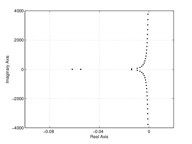
In Figure 1 we show the eigenvalue pairs corresponding to the simulation example from §4. They were obtained by application of Newton’s method to the equation (2.24).
Refer to caption
Figure 1. The eigenvalues λn\lambda_{n} of the system approach the imaginary axis as n→∞n\rightarrow\infty.
Remark 2.2.

It can also be shown that the condition (2.3) does not hold. In particular, it can be shown that there is a constant CC, a sequence {μn}⊂ℝ\{\mu_{n}\}\subset\mathbb{R} diverging to +∞+\infty, and a sequence {zn}⊂D⁡(𝒜)\{z_{n}\}\subset D(\mathcal{A}) such that

‖R⁡(i​μn,𝒜)​zn‖ℋ‖zn‖ℋ>C​μn, for all ​n​ large enough.\frac{\|R(i\mu_{n},\mathcal{A})z_{n}\|_{\mathcal{H}}}{\|z_{n}\|_{\mathcal{H}}}>C\mu_{n},\quad\text{ for all }n\text{ large enough.}

But since the details of this calculation are rather technical we only present them in [36].

Remark 2.3.

We shall now comment on the asymptotic behavior of the eigenfunctions of 𝒜\mathcal{A}. The solution to (2.15)–(2.19) for τ=τn\tau=\tau_{n} has the form (see [40]):

u~n​(y)=|γ1​(0)γ2​(0)γ3​(0)γ4​(0)(γ1)y​(0)(γ2)y​(0)(γ3)y​(0)(γ4)y​(0)m31m32m33m34γ1​(y)γ2​(y)γ3​(y)γ4​(y)|,\tilde{u}_{n}(y)=\begin{vmatrix}\gamma_{1}(0)&\gamma_{2}(0)&\gamma_{3}(0)&\gamma_{4}(0)\\ (\gamma_{1})_{y}(0)&(\gamma_{2})_{y}(0)&(\gamma_{3})_{y}(0)&(\gamma_{4})_{y}(0)\\ m_{31}&m_{32}&m_{33}&m_{34}\\ \gamma_{1}(y)&\gamma_{2}(y)&\gamma_{3}(y)&\gamma_{4}(y)\end{vmatrix},

up to a multiplicative constant. Using the Laplace expansion of the determinant and scaling the expression with e−τ​τ−6​1l1​2​ie^{-\tau}\tau^{-6}\frac{1}{l_{1}2i}, u~n\tilde{u}_{n} has the approximate form (for nn large):

u~n​(y)=e−(n−12)​π​y−cos⁡((n−12)​π​y)+sin⁡((n−12)​π​y)+(−1)n​e(n−12)​π​(y−1)+𝒪⁡(n−1),\tilde{u}_{n}(y)=e^{-(n-\frac{1}{2})\pi y}-\cos{\left((n-\frac{1}{2})\pi y\right)}+\sin{\left((n-\frac{1}{2})\pi y\right)}+(-1)^{n}e^{(n-\frac{1}{2})\pi(y-1)}+\mathcal{O}(n^{-1}),

for 0≤y≤10\leq y\leq 1. Therefore, the function unu_{n} corresponding to the eigenvalue λn\lambda_{n} has the following asymptotic property:

un​(x)\displaystyle u_{n}(x) =\displaystyle= e−14∫0yα3(z)dz[e−(n−12)​π​y−cos((n−12)πy)+sin((n−12)πy)\displaystyle e^{-\frac{1}{4}\int_{0}^{y}{\alpha_{3}(z)\,dz}}\left[e^{-(n-\frac{1}{2})\pi y}-\cos{\left((n-\frac{1}{2})\pi y\right)}+\sin{\left((n-\frac{1}{2})\pi y\right)}\right.
+(−1)ne(n−12)​π​(y−1)+𝒪(n−1)],\displaystyle\left.+(-1)^{n}e^{(n-\frac{1}{2})\pi(y-1)}+\mathcal{O}(n^{-1})\vphantom{\cos{\left((n-\frac{1}{2})\pi y\right)}}\right],

where 0≤x≤L0\leq x\leq L, with y=y⁡(x)y=y(x) and α3\alpha_{3} as in (2.11) and (2.13).

Remark 2.4.

The uncontrolled system (i.e. with A1,2=0,d1,2=0A_{1,2}=0,d_{1,2}=0) is undamped and its operator 𝒜\mathcal{A} then has purely imaginary eigenvalues. But their asymptotic behavior is still like in Theorem 3, as can be verified by the analogue of the above computation.

3. Dissipative FEM method

From Theorem 1 we know that the norm of the solution z⁡(t)z(t) decreases in time. Using (1.7), a straightforward calculation (for a classical solution) yields:

(3.1) dd​t​‖z‖ℋ2\displaystyle\frac{d}{dt}\|z\|^{2}_{\mathcal{H}} =\displaystyle= −δ1​ux​t​(L)2−12​(ζ1⋅q1+δ~1​ux​t​(L))2\displaystyle-\delta_{1}u_{xt}(L)^{2}-\frac{1}{2}\left(\zeta_{1}\cdot q_{1}+\tilde{\delta}_{1}u_{xt}(L)\right)^{2}
−δ2​ut​(L)2−12​(ζ2⋅q2+δ~2​ut​(L))2\displaystyle-\delta_{2}u_{t}(L)^{2}-\frac{1}{2}\left(\zeta_{2}\cdot q_{2}+\tilde{\delta}_{2}u_{t}(L)\right)^{2}
−ϵ12​ζ1⊤​P1​ζ1−ϵ22​ζ2⊤​P2​ζ2≤0,\displaystyle-\frac{\epsilon_{1}}{2}\zeta_{1}^{\top}P_{1}\zeta_{1}-\frac{\epsilon_{2}}{2}\zeta_{2}^{\top}P_{2}\zeta_{2}\leq 0,

where δ~j=2​(dj−δj),j=1,2.\tilde{\delta}_{j}=\sqrt{2(d_{j}-\delta_{j})},\;j=1,2. Note that the r.h.s. of (3.1) only involves boundary terms of the beam and the control variables. Hence, dd​t​‖z‖ℋ2=0\frac{d}{dt}\|z\|^{2}_{\mathcal{H}}=0 does not imply z=0z=0 (which can easily be verified from (2.1)).

The goal of this section is to derive a FEM for (1.1)–(1.5) coupled to the ODE-system (1.6) that preserves this structural property of dissipativity. The importance of this feature is twofold: For long-time computations, the numerical scheme must of course be convergent in the classical sense (i.e. on finite time intervals) but also yield the correct large-time limit. Moreover, dissipativity of the scheme implies immediately unconditional stability.

Here we shall construct first a time-continuous and then a time-discrete FEM that both dissipate the norm in time. Let us briefly discuss the different options to proceed. (2.1) is an inconvenient starting point for deriving a weak formulation due to the high boundary traces of uu at x=Lx=L: The natural regularity of a weak solution would be u∈C⁡([0,∞),H~02​(0,L))u\in C([0,\infty);\tilde{H}^{2}_{0}(0,L)), v=ut∈C⁡([0,∞),L2​(0,L))v=u_{t}\in C([0,\infty);L^{2}(0,L)). Hence, the terms Λ⁡(L)​ux​x​(t,L)\Lambda(L)u_{xx}(t,L), (Λ​ux​x)x​(t,L)(\Lambda u_{xx})_{x}(t,L) in (2.1) could only be incorporated by resorting to the boundary conditions (1.4), (1.5). Therefore we shall rather start from the original second order system (1.1)–(1.6).

3.1. Weak formulation

In order to derive the weak formulation, we assume the following initial conditions

(3.2a) u⁡(0)\displaystyle u(0) =u0∈H~02​(0,L),\displaystyle=u_{0}\in\tilde{H}_{0}^{2}(0,L),
(3.2b) ut​(0)\displaystyle u_{t}(0) =v0∈L2​(0,L),\displaystyle=v_{0}\in L^{2}(0,L),
(3.2c) ζ1​(0)\displaystyle\zeta_{1}(0) =ζ1,0∈ℝn,\displaystyle=\zeta_{1,0}\in\mathbb{R}^{n},
(3.2d) ζ2​(0)\displaystyle\zeta_{2}(0) =ζ2,0∈ℝn.\displaystyle=\zeta_{2,0}\in\mathbb{R}^{n}.

Moreover, let v0​(L)v_{0}(L) and (v0)x​(L)(v_{0})_{x}(L) be given in addition to the function v0v_{0}, and not as its trace. Multiplying (1.1) by w∈H~02​(0,L)w\in\tilde{H}^{2}_{0}(0,L), integrating over [0,L][0,L], and taking into account the given boundary conditions we obtain:

∫0Lμ​ut​t​w​𝑑x+∫0LΛ​ux​x​wx​x​𝑑x+M​ut​t​(t,L)​w​(L)+J​ut​t​x​(t,L)​wx​(L)\displaystyle\int_{0}^{L}{\mu u_{tt}w\,dx}+\int_{0}^{L}{\Lambda u_{xx}w_{xx}\,dx}+Mu_{tt}(t,L)w(L)+Ju_{ttx}(t,L)w_{x}(L)
(3.3) +k1​ux​(t,L)​wx​(L)+k2​u​(t,L)​w​(L)+d1​ut​x​(t,L)​wx​(L)+d2​ut​(t,L)​w​(L)\displaystyle+k_{1}u_{x}(t,L)w_{x}(L)+k_{2}u(t,L)w(L)+d_{1}u_{tx}(t,L)w_{x}(L)+d_{2}u_{t}(t,L)w(L)
+c1⋅ζ1(t)wx(L)+c2⋅ζ2(t)w(L)=0,∀w∈H~02(0,L),t>0.\displaystyle+c_{1}\cdot\zeta_{1}(t)\;w_{x}(L)+c_{2}\cdot\zeta_{2}(t)\;w(L)=0,\quad\quad\quad\quad\quad\forall w\in\tilde{H}^{2}_{0}(0,L),\;t>0.

This identity will motivate the weak formulation. First, we define the Hilbert space

H:=ℝ×ℝ×L2​(0,L),H:=\mathbb{R}\times\mathbb{R}\times L^{2}(0,L),

with inner product

(φ^,ν^)H\displaystyle(\hat{\varphi},\hat{\nu})_{H} :⁣=\displaystyle:= J(1φ^)(1ν^)+M(2φ^)(2ν^)+(μ3φ^,3ν^)L2,\displaystyle J\,(^{1}\hat{\varphi})\,(^{1}\hat{\nu})+M\,(^{2}\hat{\varphi})\,(^{2}\hat{\nu})+(\mu\,^{3}\hat{\varphi},\,^{3}\hat{\nu})_{L^{2}},

for φ^=(1φ^,2φ^,3φ^),ν∈H.\hat{\varphi}=(^{1}\hat{\varphi},\,^{2}\hat{\varphi},\,^{3}\hat{\varphi}),\,\nu\in H. We also define the Hilbert space

V:={w^=(wx​(L),w⁡(L),w):w∈H~02​(0,L)},V:=\{\hat{w}=(w_{x}(L),w(L),w)\colon w\in\tilde{H}^{2}_{0}(0,L)\},

with the inner product

(w1^,w2^)V=(Λ​(w1)x​x,(w2)x​x)L2.(\hat{w_{1}},\hat{w_{2}})_{V}=(\Lambda(w_{1})_{xx},(w_{2})_{xx})_{L^{2}}.

It can be shown that VV is densely embedded in HH. Therefore taking HH as a pivot space, we have the Gelfand triple

V⊂H⊂V′.V\subset H\subset V^{\prime}.

For any fixed T>0T>0 we now define u^=(ux​(L),u⁡(L),u)\hat{u}=(u_{x}(L),u(L),u) and ζ1,ζ2\zeta_{1},\zeta_{2} to be the weak solution to (1.1)–(1.6) and (3.2) if

u^∈L2​(0,T,V)∩H1​(0,T,H)∩H2​(0,T,V′),\hat{u}\in L^{2}(0,T;V)\cap H^{1}(0,T;H)\cap H^{2}(0,T;V^{\prime}),
ζ1,ζ2∈H1​(0,T,ℝn)\zeta_{1},\zeta_{2}\in H^{1}(0,T;\mathbb{R}^{n})

and it satisfies:

(3.4) V′<u^t​t,w^>V+a(u^,w^)+b(u^t,w^)+e1(ζ1,w^)+e2(ζ2,w^)=0,_{V^{\prime}}<\hat{u}_{tt},\hat{w}>_{V}+a(\hat{u},\hat{w})+b(\hat{u}_{t},\hat{w})+e_{1}(\zeta_{1},\hat{w})+e_{2}(\zeta_{2},\hat{w})=0,

for a.e. ​t∈(0,T),∀w^∈V\text{for a.e. }t\in(0,T),\forall\hat{w}\in V. The bilinear form V′<.,.>V{}_{V^{\prime}}<.,.>_{V} is the duality pairing between VV and V′V^{\prime} as a natural extension of the inner product in HH. The bilinear forms a:V×V→ℝa:V\times V\rightarrow\mathbb{R}, b:H×H→ℝb:H\times H\rightarrow\mathbb{R} and e1,e2:ℝn×V→ℝe_{1},e_{2}:\mathbb{R}^{n}\times V\rightarrow\mathbb{R} are given by

a⁡(w1^,w2^)\displaystyle a(\hat{w_{1}},\hat{w_{2}}) =\displaystyle= (w1^,w2^)V+k1​(w1)x​(L)​(w2)x​(L)+k2​w1​(L)​w2​(L),\displaystyle(\hat{w_{1}},\hat{w_{2}})_{V}+k_{1}(w_{1})_{x}(L)(w_{2})_{x}(L)+k_{2}w_{1}(L)w_{2}(L),
b⁡(φ^,ν^)\displaystyle b(\hat{\varphi},\hat{\nu}) =\displaystyle= d1(1φ^)(1ν^)+d2(2φ^)(2ν^),\displaystyle d_{1}(^{1}\hat{\varphi})(^{1}\hat{\nu})+d_{2}(^{2}\hat{\varphi})(^{2}\hat{\nu}),
e1​(ζ1,w^)\displaystyle e_{1}(\zeta_{1},\hat{w}) =\displaystyle= c1⋅ζ1​wx​(L),\displaystyle c_{1}\cdot\zeta_{1}w_{x}(L),
e2​(ζ2,w^)\displaystyle e_{2}(\zeta_{2},\hat{w}) =\displaystyle= c2⋅ζ2​w​(L).\displaystyle c_{2}\cdot\zeta_{2}w(L).

Equation (3.4) is coupled to the ODEs

(ζ1)t​(t)=A1ζ1(t)+b1(1u^t(t)),(ζ2)t​(t)=A2ζ2(t)+b2(2u^t(t)),\displaystyle\begin{array}[]{rcl}(\zeta_{1})_{t}(t)&=&A_{1}\zeta_{1}(t)+b_{1}\,(^{1}\hat{u}_{t}(t)),\\ (\zeta_{2})_{t}(t)&=&A_{2}\zeta_{2}(t)+b_{2}\,(^{2}\hat{u}_{t}(t)),\end{array}

with initial conditions

(3.8a) u^​(0)\displaystyle\hat{u}(0) =u^0=((u0)x​(L),u0​(L),u0)∈V,\displaystyle=\hat{u}_{0}=((u_{0})_{x}(L),u_{0}(L),u_{0})\in V,
(3.8b) u^t​(0)\displaystyle\hat{u}_{t}(0) =v^0=((v0)x​(L),v0​(L),v0)∈H,\displaystyle=\hat{v}_{0}=((v_{0})_{x}(L),v_{0}(L),v_{0})\in H,
(3.8c) ζ1​(0)\displaystyle\zeta_{1}(0) =ζ1,0∈ℝn,\displaystyle=\zeta_{1,0}\in\mathbb{R}^{n},
(3.8d) ζ2​(0)\displaystyle\zeta_{2}(0) =ζ2,0∈ℝn.\displaystyle=\zeta_{2,0}\in\mathbb{R}^{n}.

In (3.8a) the first two components of the right hand side are the boundary traces of u0∈H~02​(0,L)u_{0}\in\tilde{H}^{2}_{0}(0,L), but in (3.8b) they are additionally given values. Note that in the case when u^∈H2​(0,T,V)\hat{u}\in H^{2}(0,T;V), formulation (3.4) is equivalent to identity (3.3). This weak formulation is an extension of [4](Section 2) to the case where the beam with the tip-mass is additionally coupled to the first order ODE controller system. Here, we have to deal also with ut​(L)u_{t}(L) and ut​x​(L)u_{tx}(L). And these additional first order boundary terms (in tt), included in b(.,.)b(.,.), require a slight generalization of the standard theory (as presented in §8 of [33], e.g.).

In order to give a meaning to the initial conditions (3.8a), (3.8b) we shall use the following lemma (special case of Theorem 3.1 in [33]).

Lemma 3.1.

Let XX and YY be two Hilbert spaces, such that XX is dense and continuously embedded in YY. Assume that

u\displaystyle u ∈\displaystyle\in L2​(0,T,X),\displaystyle L^{2}(0,T;X),
ut\displaystyle u_{t} ∈\displaystyle\in L2​(0,T,Y).\displaystyle L^{2}(0,T;Y).

Then

u∈C([0,T];[X,Y]12]),u\in C([0,T];[X,Y]_{\frac{1}{2}}]),

after, possibly, a modification on a set of measure zero. Here, the definition of intermediate spaces as given in [33], §2.1, was assumed.

Theorem 4.
  1. (a)

    The weak formulation (3.4) – (3.8) has a unique solution (u^,ζ1,ζ2)(\hat{u},\zeta_{1},\zeta_{2}).

  2. (b)

    The weak solution has the additional regularity

    (3.9a) u^∈L∞​(0,T,V),u^t∈L∞​(0,T,H),\displaystyle\hat{u}\in L^{\infty}(0,T;V),\quad\hat{u}_{t}\in L^{\infty}(0,T;H),
    (3.9b) ζ1,ζ2∈C⁡([0,T],ℝn),\displaystyle\zeta_{1},\zeta_{2}\in C([0,T];\mathbb{R}^{n}),
    (3.9c) u^∈C⁡([0,T],[V,H]12),\displaystyle\hat{u}\in C([0,T];[V,H]_{\frac{1}{2}}),
    (3.9d) u^t∈C([0,T];[V,H]12′).\displaystyle\hat{u}_{t}\in C([0,T];[V,H]_{\frac{1}{2}}^{{}^{\prime}}).

Furthermore, even stronger continuity for the weak solution can be shown:

Theorem 5.

After, possibly, a modification on a set of measure zero, the weak solution u^\hat{u} of (3.4)-(3.8) satisfies

u^\displaystyle\hat{u} ∈\displaystyle\in C⁡([0,T],V),\displaystyle C([0,T];V),
u^t\displaystyle\hat{u}_{t} ∈\displaystyle\in C⁡([0,T],H).\displaystyle C([0,T];H).

The proofs of Theorem 4 and 5 are given in Appendix A.

3.2. Semi-discrete scheme: space discretization

Now let Wh⊂H~02​(0,L)W_{h}\subset\tilde{H}_{0}^{2}(0,L) be a finite dimensional space. Its elements are globally C1​[0,L]C^{1}[0,L], due to a Sobolev embedding. For some fixed basis wj,j=1,…,Nw_{j},j=1,\dots,N the Galerkin approximation of (3.4) reads: Find uh∈C2​([0,∞),Wh)u_{h}\in C^{2}([0,\infty),W_{h}), i.e. u^h=((uh)x​(L),uh​(L),uh)∈C2​([0,∞),V)\hat{u}_{h}=((u_{h})_{x}(L),u_{h}(L),u_{h})\in C^{2}([0,\infty),V), and ζ~1,2∈C1​([0,∞),ℝn)\tilde{\zeta}_{1,2}\in C^{1}([0,\infty),\mathbb{R}^{n}) with

(3.10) ∫0Lμ​(uh)t​t​wj​𝑑x+∫0LΛ​(uh)x​x​(wj)x​x​𝑑x+M​(uh)t​t​(t,L)​wj​(L)+J​(uh)x​t​t​(t,L)​(wj)x​(L)+k1​(uh)x​(t,L)​(wj)x​(L)+k2​uh​(t,L)​wj​(L)+d1​(uh)x​t​(t,L)​(wj)x​(L)+d2​(uh)t​(t,L)​(wj)​(L)+c1⋅ζ~1(t)(wj)x(L)+c2⋅ζ~2(t)wj(L)=0,j=1,…,N,t>0,\begin{array}[]{ccl}&&\int_{0}^{L}{\mu(u_{h})_{tt}w_{j}\,dx}+\int_{0}^{L}{\Lambda(u_{h})_{xx}(w_{j})_{xx}\,dx}\\ &&+M(u_{h})_{tt}(t,L)w_{j}(L)+J(u_{h})_{xtt}(t,L)(w_{j})_{x}(L)\\ &&+k_{1}(u_{h})_{x}(t,L)(w_{j})_{x}(L)+k_{2}u_{h}(t,L)w_{j}(L)\\ &&+d_{1}(u_{h})_{xt}(t,L)(w_{j})_{x}(L)+d_{2}(u_{h})_{t}(t,L)(w_{j})(L)\\ &&+c_{1}\cdot\tilde{\zeta}_{1}(t)\;(w_{j})_{x}(L)+c_{2}\cdot\tilde{\zeta}_{2}(t)\;w_{j}(L)=0,\quad\quad\quad j=1,\dots,N,\;t>0,\end{array}

coupled to the analogue of (3.1):

(ζ~1)t​(t)=A1​ζ~1​(t)+b1​(uh)x​t​(t,L),(ζ~2)t​(t)=A2​ζ~2​(t)+b2​(uh)t​(t,L),\displaystyle\begin{array}[]{rcl}(\tilde{\zeta}_{1})_{t}(t)&=&A_{1}\tilde{\zeta}_{1}(t)+b_{1}(u_{h})_{xt}(t,L),\\ (\tilde{\zeta}_{2})_{t}(t)&=&A_{2}\tilde{\zeta}_{2}(t)+b_{2}(u_{h})_{t}(t,L),\end{array}

and the initial conditions

uh​(0,.)\displaystyle u_{h}(0,\ldotp) =\displaystyle= uh,0∈Wh,\displaystyle u_{h,0}\in W_{h},
(uh)t​(0,.)\displaystyle(u_{h})_{t}(0,\ldotp) =\displaystyle= vh,0∈Wh,\displaystyle v_{h,0}\in W_{h},
ζ~1​(0)\displaystyle\tilde{\zeta}_{1}(0) =\displaystyle= ζ1,0∈ℝn,\displaystyle\zeta_{1,0}\in\mathbb{R}^{n},
ζ~2​(0)\displaystyle\tilde{\zeta}_{2}(0) =\displaystyle= ζ2,0∈ℝn.\displaystyle\zeta_{2,0}\in\mathbb{R}^{n}.

(3.10) is a second order ODE-system in time. Expanding its solution in the chosen basis, i.e.

uh​(t,x)=∑i=1NUi​(t)​wi​(x),u_{h}(t,x)=\sum_{i=1}^{N}{U_{i}(t)w_{i}(x)},

and denoting its coefficients by the vector

𝕌=[U1U2…UN]⊤\mathbb{U}=\left[\begin{array}[]{c c c c}U_{1}&U_{2}&\dots&U_{N}\end{array}\right]^{\top}

yields the equivalent vector equation:

(3.14) 𝔸​𝕌t​t+𝔹​𝕌t+𝕂​𝕌+ℂ⁡(t)=0.\mathbb{A}\mathbb{U}_{tt}+\mathbb{B}\mathbb{U}_{t}+\mathbb{K}\mathbb{U}+\mathbb{C}(t)=0.

Its coefficient matrices are defined as

𝔸i,j\displaystyle\mathbb{A}_{i,j} :⁣=\displaystyle:= ∫0Lμ​wi​wj​𝑑x+M​wi​(L)​wj​(L)+J​(wi)x​(L)​(wj)x​(L),\displaystyle\int_{0}^{L}{\mu\,w_{i}w_{j}\,dx}+Mw_{i}(L)w_{j}(L)+J(w_{i})_{x}(L)(w_{j})_{x}(L),
𝔹i,j\displaystyle\mathbb{B}_{i,j} :⁣=\displaystyle:= d1​(wi)x​(L)​(wj)x​(L)+d2​wi​(L)​wj​(L),\displaystyle d_{1}(w_{i})_{x}(L)(w_{j})_{x}(L)+d_{2}w_{i}(L)w_{j}(L),
𝕂i,j\displaystyle\mathbb{K}_{i,j} :⁣=\displaystyle:= ∫0LΛ​(wi)x​x​(wj)x​x​𝑑x+k1​(wi)x​(L)​(wj)x​(L)+k2​wi​(L)​wj​(L),\displaystyle\int_{0}^{L}{\Lambda(w_{i})_{xx}(w_{j})_{xx}\,dx}+k_{1}(w_{i})_{x}(L)(w_{j})_{x}(L)+k_{2}w_{i}(L)w_{j}(L),
i,j=1,…,N,\displaystyle i,j=1,\dots,N,

and the vector ℂ\mathbb{C} has the entries

ℂj(t)=c1⋅ζ~1(t)(wj)x(L)+c2⋅ζ~2(t)wj(L),j=1,…,N.\mathbb{C}_{j}(t)=c_{1}\cdot\tilde{\zeta}_{1}(t)\;(w_{j})_{x}(L)+c_{2}\cdot\tilde{\zeta}_{2}(t)\;w_{j}(L),\quad j=1,\dots,N.

The matrix 𝕂\mathbb{K} is symmetric positive definite, since we assumed k1,2>0k_{1,2}>0. Since also 𝔸\mathbb{A} is symmetric positive definite, one sees very easily that the IVP corresponding to the coupled problem (3.14), (3.2) is uniquely solvable.

For a final specification of the FEM we need to choose an appropriate discrete space. Only for notational simplicity, we shall assume a uniform distribution of nodes on [0,L][0,L]:

xm=m​h,m∈{0,1,…,P},x_{m}=mh,\quad m\in\{0,1,\dots,P\},

where h=LP.h=\frac{L}{P}. A standard choice for the discrete space WhW_{h} is a space of piecewise cubic polynomials with both displacement and slope continuity across element boundaries, also called Hermitian cubic polynomials (see [44], [6], e.g.). They have been employed not only for the Euler-Bernoulli beam, but also Timoshenko beams (cf. [17]). To define a basis for WhW_{h} (Hermite cubic basis, see e.g. [43]), we associate two piecewise cubic functions with each node xm,m≥1x_{m},\;m\geq 1 satisfying:

w2​m−1​(xk)={1,m=k0,m≠k\displaystyle w_{2m-1}(x_{k})=\left\{\begin{array}[]{c l}1,&m=k\\ 0,&m\neq k\end{array}\right. w2​m−1′​(xk)=0,\displaystyle w^{\prime}_{2m-1}(x_{k})=0,
w2​m′​(xk)={1,m=k0,m≠k\displaystyle w^{\prime}_{2m}(x_{k})=\left\{\begin{array}[]{c l}1,&m=k\\ 0,&m\neq k\end{array}\right. w2​m​(xk)=0,\displaystyle w_{2m}(x_{k})=0,

for all k=0,…,Pk=0,\dots,P. Hence, the nodal values of a function and of its derivative are the associated degrees of freedom. Due to the boundary conditions at x=0x=0 in Wh⊂H~02W_{h}\subset\tilde{H}_{0}^{2}, the basis set does not include the functions w−1w_{-1} and w0w_{0} associated to the node x0=0x_{0}=0. Thus, N=2​PN=2P. For the coupling to the control variables we shall need the boundary values of uhu_{h}. The above basis yields the simple relations uh​(t,L)=UN−1​(t),(uh)x​(t,L)=UN​(t)u_{h}(t,L)=U_{N-1}(t),\;(u_{h})_{x}(t,L)=U_{N}(t). Compact support of the basis functions {wj}j=1N\{w_{j}\}_{j=1}^{N} leads to a sparse structure of the matrices 𝔸\mathbb{A}, 𝔹\mathbb{B}, and 𝕂\mathbb{K}: 𝔸\mathbb{A} and 𝕂\mathbb{K} are tridiagonal, 𝔹\mathbb{B} is diagonal with only two non-zero elements 𝔹N−1,N−1=d2\mathbb{B}_{N-1,N-1}=d_{2}, 𝔹N,N=d1\mathbb{B}_{N,N}=d_{1}. And the vector ℂ\mathbb{C} has all zero entries except for ℂN−1=c2⋅ζ2~\mathbb{C}_{N-1}=c_{2}\cdot\tilde{\zeta_{2}}, ℂN=c1⋅ζ1~\mathbb{C}_{N}=c_{1}\cdot\tilde{\zeta_{1}}.

Next, we shall show that the semi-discrete solution uh​(t)u_{h}(t) decreases in time. As an analogue of the norm ‖z⁡(t)‖ℋ\|z(t)\|_{\mathcal{H}} from §2, we first define the following time dependent functional for a trajectory u∈C2​([0,∞),H~02​(0,L))u\in C^{2}([0,\infty);\tilde{H}^{2}_{0}(0,L)) and ζ1,2∈C1​([0,∞),ℝn)\zeta_{1,2}\in C^{1}([0,\infty);\mathbb{R}^{n}):

(3.17) E⁡(t,u,ζ1,ζ2)\displaystyle E(t;u,\zeta_{1},\zeta_{2}) :=\displaystyle\!\!:=\!\! 12​∫0L(Λ​ux​x​(t,x)2+μ​ut​(t,x)2)​𝑑x+M2​ut​(t,L)2+J2​ux​t​(t,L)2\displaystyle\frac{1}{2}\int_{0}^{L}\left(\Lambda u_{xx}(t,x)^{2}+\mu u_{t}(t,x)^{2}\right)\,dx+\frac{M}{2}u_{t}(t,L)^{2}+\frac{J}{2}u_{xt}(t,L)^{2}
+k12​ux​(t,L)2+k22​u​(t,L)2+12​ζ1⊤​(t)​P1​ζ1​(t)+12​ζ2⊤​(t)​P2​ζ2​(t).\displaystyle+\frac{k_{1}}{2}u_{x}(t,L)^{2}+\frac{k_{2}}{2}u(t,L)^{2}+\frac{1}{2}\zeta_{1}^{\top}(t)P_{1}\zeta_{1}(t)+\frac{1}{2}\zeta_{2}^{\top}(t)P_{2}\zeta_{2}(t).

For a classical solution of (2.1) in D⁡(𝒜)D(\mathcal{A}) we have E⁡(t,u,ζ1,ζ2)=‖z⁡(t)‖ℋ2E(t;u,\zeta_{1},\zeta_{2})=\|z(t)\|_{\mathcal{H}}^{2}.

Theorem 6.

Let uh∈C2​([0,∞),H~02​(0,L))u_{h}\in C^{2}([0,\infty);\tilde{H}^{2}_{0}(0,L)) and ζ~1,2∈C1​([0,∞),ℝn)\tilde{\zeta}_{1,2}\in C^{1}([0,\infty);\mathbb{R}^{n}) solve (3.10), (3.2). Then it holds for t>0t>0:

dd​t​E​(t,uh,ζ~1,ζ~2)\displaystyle\frac{d}{dt}E(t;u_{h},\tilde{\zeta}_{1},\tilde{\zeta}_{2}) =\displaystyle= −ϵ12​ζ~1⊤​P1​ζ~1−12​(ζ~1⋅q1+δ~1​(uh)x​t​(L))2−δ1​(uh)x​t​(L)2\displaystyle-\frac{\epsilon_{1}}{2}\tilde{\zeta}_{1}^{\top}P_{1}\tilde{\zeta}_{1}-\frac{1}{2}\left(\tilde{\zeta}_{1}\cdot q_{1}+\tilde{\delta}_{1}(u_{h})_{xt}(L)\right)^{2}-\delta_{1}(u_{h})_{xt}(L)^{2}
−ϵ22​ζ~2⊤​P2​ζ~2−12​(ζ~2⋅q2+δ~2​(uh)t​(L))2−δ2​(uh)t​(L)2≤0.\displaystyle-\frac{\epsilon_{2}}{2}\tilde{\zeta}_{2}^{\top}P_{2}\tilde{\zeta}_{2}-\frac{1}{2}\left(\tilde{\zeta}_{2}\cdot q_{2}+\tilde{\delta}_{2}(u_{h})_{t}(L)\right)^{2}-\delta_{2}(u_{h})_{t}(L)^{2}\leq 0.
Proof.

In the following computation we use (3.10) with the test function wh=(uh)tw_{h}=(u_{h})_{t}:

dd​t​E​(t,uh,ζ~1,ζ~2)\displaystyle\frac{d}{dt}E(t;u_{h},\tilde{\zeta}_{1},\tilde{\zeta}_{2}) =\displaystyle= ∫0LΛ​(uh)x​x​(uh)x​x​t​𝑑x+∫0Lμ​(uh)t​(uh)t​t​𝑑x\displaystyle\int_{0}^{L}{\Lambda(u_{h})_{xx}(u_{h})_{xxt}\,dx}+\int_{0}^{L}{\mu(u_{h})_{t}(u_{h})_{tt}\,dx}
+M​(uh)t​(L)​(uh)t​t​(L)+J​(uh)t​x​(L)​(uh)t​t​x​(L)\displaystyle+M(u_{h})_{t}(L)(u_{h})_{tt}(L)+J(u_{h})_{tx}(L)(u_{h})_{ttx}(L)
+k1​(uh)x​(L)​(uh)x​t​(L)+k2​(uh)​(L)​(uh)t​(L)\displaystyle+k_{1}(u_{h})_{x}(L)(u_{h})_{xt}(L)+k_{2}(u_{h})(L)(u_{h})_{t}(L)
+ζ~1⊤​P1​(ζ~1)t+ζ~2⊤​P2​(ζ~2)t\displaystyle+\tilde{\zeta}_{1}^{\top}P_{1}(\tilde{\zeta}_{1})_{t}+\tilde{\zeta}_{2}^{\top}P_{2}(\tilde{\zeta}_{2})_{t}
=\displaystyle= −d1​(uh)x​t​(L)2−d2​(uh)t​(L)2\displaystyle-d_{1}(u_{h})_{xt}(L)^{2}-d_{2}(u_{h})_{t}(L)^{2}
−c1⋅ζ~1(uh)x​t(L)−c2⋅ζ~2(uh)t(L)+ζ~1⊤P1(ζ~1)t+ζ~2⊤P2(ζ~2)t,\displaystyle-c_{1}\cdot\tilde{\zeta}_{1}(u_{h})_{xt}(L)-c_{2}\cdot\tilde{\zeta}_{2}(u_{h})_{t}(L)+\tilde{\zeta}_{1}^{\top}P_{1}(\tilde{\zeta}_{1})_{t}+\tilde{\zeta}_{2}^{\top}P_{2}(\tilde{\zeta}_{2})_{t},

and the result follows with (3.2) and (1.7). ∎

In the undamped case (i.e. Aj=0,dj=0A_{j}=0,d_{j}=0) the energy EE is clearly preserved in the semi-discrete system. Furthermore, it has been shown in the proof of Theorem 5 that the energy functional for the weak solution u^\hat{u}, ζ1,ζ2\zeta_{1},\zeta_{2} of (3.4) - (3.8) has an analogous dissipative property, cf. (5.15).

3.3. Error estimates: semi-discrete scheme

Since using cubic polynomials for the space approximation, we shall obtain accuracy of order two in space (in H2​(0,L)H^{2}(0,L)). Thereby, the common method for obtaining error estimates (cf. [13]) will be adjusted to the problem at hand. With u~\tilde{u} we denote the nodal projection of the weak solution uu to WhW_{h}, defined in terms of Hermite polynomials:

u~​(t,x)\displaystyle\tilde{u}(t,x) =\displaystyle= ∑m=1Pu⁡(t,xm)​w2​m−1​(x)+∑m=1Pux​(t,xm)​w2​m​(x).\displaystyle\sum_{m=1}^{P}{u(t,x_{m})w_{2m-1}(x)}+\sum_{m=1}^{P}{u_{x}(t,x_{m})w_{2m}(x)}.

Assuming that

(3.18) u∈C⁡([0,T],H~04​(0,L)),ut∈L2​(0,T,H~04​(0,L)),ut​t∈L2​(0,T,H~02​(0,L)),\begin{array}[]{l}u\in C([0,T];\tilde{H}_{0}^{4}(0,L)),\\ u_{t}\in L^{2}(0,T;\tilde{H}_{0}^{4}(0,L)),\\ u_{tt}\in L^{2}(0,T;\tilde{H}_{0}^{2}(0,L)),\end{array}

it can be seen (e.g. in [7], [13]) that a.e. in tt:

(3.19) ‖u−u~‖H2​(0,L)≤C​h2​‖u‖H4​(0,L),‖ut−u~t‖H2​(0,L)≤C​h2​‖ut‖H4​(0,L),‖ut​t−u~t​t‖L2​(0,L)≤C​h2​‖ut​t‖H2​(0,L).\begin{array}[]{r c l}\|u-\tilde{u}\|_{H^{2}(0,L)}&\leq&Ch^{2}\|u\|_{H^{4}(0,L)},\\ \|u_{t}-\tilde{u}_{t}\|_{H^{2}(0,L)}&\leq&Ch^{2}\|u_{t}\|_{H^{4}(0,L)},\\ \|u_{tt}-\tilde{u}_{tt}\|_{L^{2}(0,L)}&\leq&Ch^{2}\|u_{tt}\|_{H^{2}(0,L)}.\end{array}

We define the error of the semi-discrete solution (uh,ζ~1,ζ~2)(u_{h},\tilde{\zeta}_{1},\tilde{\zeta}_{2}) as ϵh:=uh−u~∈Wh\epsilon_{h}:=u_{h}-\tilde{u}\in W_{h} and ζei:=ζ~i−ζi,i=1,2.\zeta^{e}_{i}:=\tilde{\zeta}_{i}-\zeta_{i},\;i=1,2. Then using (3.10)–(3.2) we obtain

∫0Lμ​(ϵh)t​t​w​𝑑x+∫0LΛ​(ϵh)x​x​wx​x​𝑑x+M​(ϵh)t​t​(t,L)​w​(L)+J​(ϵh)x​t​t​(t,L)​wx​(L)+k1​(ϵh)x​(t,L)​wx​(L)+k2​ϵh​(t,L)​w​(L)+d1​(ϵh)x​t​(t,L)​wx​(L)+d2​(ϵh)t​(t,L)​w​(L)+c1⋅ζe1(t)wx(L)+c2⋅ζe2(t)w(L)=∫0Lμ(ut​t−u~t​t)wdx+∫0LΛ(ux​x−u~x​x)wx​xdx,∀w∈Wh,t>0,\begin{array}[]{ccl}&&\int_{0}^{L}{\mu(\epsilon_{h})_{tt}w\,dx}+\int_{0}^{L}{\Lambda(\epsilon_{h})_{xx}w_{xx}\,dx}\\ &&+M(\epsilon_{h})_{tt}(t,L)w(L)+J(\epsilon_{h})_{xtt}(t,L)w_{x}(L)\\ &&+k_{1}(\epsilon_{h})_{x}(t,L)w_{x}(L)+k_{2}\epsilon_{h}(t,L)w(L)\\ &&+d_{1}(\epsilon_{h})_{xt}(t,L)w_{x}(L)+d_{2}(\epsilon_{h})_{t}(t,L)w(L)\\ &&+c_{1}\cdot\zeta^{e}_{1}(t)\;w_{x}(L)+c_{2}\cdot\zeta^{e}_{2}(t)\;w(L)\\ &&=\int_{0}^{L}{\mu(u_{tt}-\tilde{u}_{tt})w\,dx}+\int_{0}^{L}{\Lambda(u_{xx}-\tilde{u}_{xx})w_{xx}\,dx},\quad\quad\quad\forall w\in W_{h},\;t>0,\end{array}

coupled to:

(ζ1e)t​(t)=A1​ζ1e​(t)+b1​(ϵh)x​t​(t,L),(ζ2e)t​(t)=A2​ζ2e​(t)+b2​(ϵh)t​(t,L).\displaystyle\begin{array}[]{rcl}(\zeta^{e}_{1})_{t}(t)&=&A_{1}\zeta^{e}_{1}(t)+b_{1}(\epsilon_{h})_{xt}(t,L),\\ (\zeta^{e}_{2})_{t}(t)&=&A_{2}\zeta^{e}_{2}(t)+b_{2}(\epsilon_{h})_{t}(t,L).\end{array}

Using w=(ϵh)tw=(\epsilon_{h})_{t} and proceeding as in the proof of Theorem 6 we obtain

(3.21) 12​dd​t​E​(t,ϵh,ζ1e,ζ2e)≤∫0Lμ⁡(ut​t−u~t​t)​(ϵh)t​dx+∫0LΛ⁡(ux​x−u~x​x)​(ϵh)t​x​x​dx,\begin{array}[]{l c l}\frac{1}{2}\frac{d}{dt}E(t;\epsilon_{h},\zeta^{e}_{1},\zeta^{e}_{2})&\leq&\int_{0}^{L}{\mu(u_{tt}-\tilde{u}_{tt})(\epsilon_{h})_{t}\,dx}+\int_{0}^{L}{\Lambda(u_{xx}-\tilde{u}_{xx})(\epsilon_{h})_{txx}\,dx},\end{array}

for a.e. t∈[0,T]t\in[0,T]. Integrating (3.21) in time, and performing partial integration, we get

(3.22) E⁡(t,ϵh,ζ1e,ζ2e)≤E⁡(0,ϵh​(0),ζ1e​(0),ζ2e​(0))+2​∫0t∫0Lμ⁡(ut​t​(s,x)−u~t​t​(s,x))​(ϵh)t​(s,x)​𝑑x​𝑑s+2​∫0LΛ⁡(ux​x​(t,x)−u~x​x​(t,x))​(ϵh)x​x​(t,x)​𝑑x+2​∫0LΛ⁡(ux​x​(0,x)−u~x​x​(0,x))​(ϵh)x​x​(0,x)​𝑑x−2​∫0t∫0LΛ⁡(ut​x​x​(s,x)−u~t​x​x​(s,x))​(ϵh)x​x​(s,x)​dx​ds.\begin{array}[]{r c l}E(t;\epsilon_{h},\zeta^{e}_{1},\zeta^{e}_{2})&\leq&E(0;\epsilon_{h}(0),\zeta^{e}_{1}(0),\zeta^{e}_{2}(0))\\ &+&2\int_{0}^{t}{\int_{0}^{L}{\mu(u_{tt}(s,x)-\tilde{u}_{tt}(s,x))(\epsilon_{h})_{t}(s,x)\,dx}\,ds}\\ &+&2\int_{0}^{L}{\Lambda(u_{xx}(t,x)-\tilde{u}_{xx}(t,x))(\epsilon_{h})_{xx}(t,x)\,dx}\\ &+&2\int_{0}^{L}{\Lambda(u_{xx}(0,x)-\tilde{u}_{xx}(0,x))(\epsilon_{h})_{xx}(0,x)\,dx}\\ &-&2\int_{0}^{t}{\int_{0}^{L}{\Lambda(u_{txx}(s,x)-\tilde{u}_{txx}(s,x))(\epsilon_{h})_{xx}(s,x)\,dx}\,ds}.\\ \end{array}

Applying Chauchy-Schwarz to (3.22) yields:

(3.23) E⁡(t,ϵh,ζ1e,ζ2e)≤E⁡(0,ϵh​(0),ζ1e​(0),ζ2e​(0))+μm​a​x(∥ut​t−u~t​t∥2L2​(0,T,L2​(0,L))+∫0t∥(ϵh)t(s,.)∥2L2​(0,L)ds)+Λm​a​x(8∥ux​x(t,.)−u~x​x(t,.)∥L2​(0,L)2+18∥(ϵh)x​x(t,.)∥L2​(0,L)2+8∥ux​x(0,.)−u~x​x(0,.)∥L2​(0,L)2+18∥(ϵh)x​x(0,.)∥L2​(0,L)2+∥ut−u~t∥2L2​(0,T,H2​(0,L))+∫0t∥(ϵh)x​x(s,.)∥2L2​(0,L)ds),\begin{array}[]{r c l}E(t;\epsilon_{h},\zeta^{e}_{1},\zeta^{e}_{2})&\leq&E(0;\epsilon_{h}(0),\zeta^{e}_{1}(0),\zeta^{e}_{2}(0))\\ &+\mu_{max}&\left(\|u_{tt}-\tilde{u}_{tt}\|^{2}_{L^{2}(0,T;L^{2}(0,L))}+\int_{0}^{t}{\|(\epsilon_{h})_{t}(s,.)\|^{2}_{L^{2}(0,L)}\,ds}\right)\\ &+\Lambda_{max}&\left(8\|u_{xx}(t,.)-\tilde{u}_{xx}(t,.)\|_{L^{2}(0,L)}^{2}+\frac{1}{8}\|(\epsilon_{h})_{xx}(t,.)\|_{L^{2}(0,L)}^{2}\right.\\ &&+8\|u_{xx}(0,.)-\tilde{u}_{xx}(0,.)\|_{L^{2}(0,L)}^{2}+\frac{1}{8}\|(\epsilon_{h})_{xx}(0,.)\|_{L^{2}(0,L)}^{2}\\ &&+\left.\|u_{t}-\tilde{u}_{t}\|^{2}_{L^{2}(0,T;H^{2}(0,L))}+\int_{0}^{t}{\|(\epsilon_{h})_{xx}(s,.)\|^{2}_{L^{2}(0,L)}\,ds}\right),\end{array}

where μm​a​x=maxx∈[0,L]⁡μ⁡(x)\mu_{max}=\max_{x\in[0,L]}{\mu(x)} and Λm​a​x=maxx∈[0,L]⁡Λ⁡(x)\Lambda_{max}=\max_{x\in[0,L]}{\Lambda(x)}. Next, we use (3.19) to obtain:

(3.24) 34​E​(t,ϵh,ζ1e,ζ2e)≤54​E​(0,ϵh​(0),ζ1e​(0),ζ2e​(0))+2​∫0tE⁡(s,ϵh,ζ1e,ζ2e)​𝑑s+C​h4​(‖u‖C⁡([0,T],H4​(0,L))2+‖ut‖L2​(0,T,H4​(0,L))2+‖ut​t‖L2​(0,T,H2​(0,L))2).\begin{array}[]{r c l}&&\frac{3}{4}E(t;\epsilon_{h},\zeta^{e}_{1},\zeta^{e}_{2})\leq\frac{5}{4}E(0;\epsilon_{h}(0),\zeta^{e}_{1}(0),\zeta^{e}_{2}(0))+2\int_{0}^{t}{E(s;\epsilon_{h},\zeta^{e}_{1},\zeta^{e}_{2})\,ds}\\ &&+Ch^{4}\left(\|u\|_{C([0,T];H^{4}(0,L))}^{2}+\|u_{t}\|^{2}_{L^{2}(0,T;H^{4}(0,L))}+\|u_{tt}\|^{2}_{L^{2}(0,T;H^{2}(0,L))}\right).\end{array}

Gronwall inequality applied to (3.24) gives:

(3.25) E⁡(t,ϵh,ζ1e,ζ2e)≤C⁡(E⁡(0,ϵh​(0),ζ1​e​(0),ζ2​e​(0))CLOSEOPEN+h4​(‖u‖C⁡([0,T],H4​(0,L))2+‖ut‖L2​(0,T,H4​(0,L))2+‖ut​t‖L2​(0,T,H2​(0,L))2)).\begin{array}[]{l}E(t;\epsilon_{h},\zeta^{e}_{1},\zeta^{e}_{2})\leq C\left(\vphantom{E^{\frac{1}{2}}}E(0;\epsilon_{h}(0),\zeta_{1e}(0),\zeta_{2e}(0))\right.\\ +\left.\vphantom{E^{\frac{1}{2}}}h^{4}\left(\|u\|^{2}_{C([0,T];H^{4}(0,L))}+\|u_{t}\|^{2}_{L^{2}(0,T;H^{4}(0,L))}+\|u_{tt}\|^{2}_{L^{2}(0,T;H^{2}(0,L))}\right)\right).\end{array}

Finally, we have:

Theorem 7.

Assuming (3.18), the following error estimate of the semidiscrete solution holds:

E​(t,uh−u,ζ~1−ζ1,ζ~2−ζ2)12≤C⁡(E​(0,ϵh​(0),ζ1​e​(0),ζ2​e​(0))12CLOSE\displaystyle E(t;u_{h}-u,\tilde{\zeta}_{1}-\zeta_{1},\tilde{\zeta}_{2}-\zeta_{2})^{\frac{1}{2}}\leq C\left(E(0;\epsilon_{h}(0),\zeta_{1e}(0),\zeta_{2e}(0))^{\frac{1}{2}}\right.
(3.26) OPEN+h2​(‖ut​t‖L2​(0,T,H2​(0,L))+‖ut‖L2​(0,T,H4​(0,L))+‖u‖C⁡([0,T],H4​(0,L)))),\displaystyle+\left.\vphantom{E^{\frac{1}{2}}}h^{2}\left(\|u_{tt}\|_{L^{2}(0,T;H^{2}(0,L))}+\|u_{t}\|_{L^{2}(0,T;H^{4}(0,L))}+\|u\|_{C([0,T];H^{4}(0,L))}\right)\right),

0≤t≤T0\leq t\leq T.

Proof.

The result follows from (3.19), (3.25), and the triangle inequality. ∎

3.4. Fully discrete scheme: time discretization

For the numerical solution to the ODE (3.14) we first write it as a first order system and then use the Crank-Nicolson scheme, which is crucial for the dissipativity of the scheme. To this end we introduce vh:=(uh)tv_{h}:=(u_{h})_{t}, and 𝕍:=𝕌t=[V1​V2​…​VN]⊤\mathbb{V}:=\mathbb{U}_{t}=[\>V_{1}\>\>V_{2}\>\>...\>\>V_{N}\>]^{\top} is its representation in the basis {wj}\{w_{j}\}. The solution of the system (3.10), (3.2) is then the vector zh=[uh​vh​ζ~1​ζ~2]⊤z_{h}=[\>u_{h}\;\>v_{h}\;\>\tilde{\zeta}_{1}\;\>\tilde{\zeta}_{2}\>]^{\top}. In contrast to §2, here we do not have to include the boundary traces vh​(L),(vh)x​(L)v_{h}(L),\,(v_{h})_{x}(L): In the finite dimensional case both uhu_{h} and vhv_{h} are in H~02​(0,L)\tilde{H}_{0}^{2}(0,L). In analogy to §2, the natural norm of zh=zh​(t)z_{h}=z_{h}(t) is defined as

(3.27) ‖zh‖2\displaystyle\|z_{h}\|^{2} :⁣=\displaystyle:= 12​∫0LΛ​(uh)x​x2​𝑑x+12​∫0Lμ​vh2​𝑑x+M2​vh2​(L)+J2​(vh)x2​(L)\displaystyle\frac{1}{2}\int_{0}^{L}{\Lambda(u_{h})_{xx}^{2}\,dx}+\frac{1}{2}\int_{0}^{L}{\mu v_{h}^{2}\,dx}+\frac{M}{2}v_{h}^{2}(L)+\frac{J}{2}(v_{h})_{x}^{2}(L)
+k12​(uh)x2​(L)+k22​uh2​(L)+12​ζ~1⊤​P1​ζ~1+12​ζ~2⊤​P2​ζ~2.\displaystyle+\frac{k_{1}}{2}(u_{h})_{x}^{2}(L)+\frac{k_{2}}{2}u_{h}^{2}(L)+\frac{1}{2}\tilde{\zeta}_{1}^{\top}P_{1}\tilde{\zeta}_{1}+\frac{1}{2}\tilde{\zeta}_{2}^{\top}P_{2}\tilde{\zeta}_{2}.

Let Δ​t\Delta t denote the time step and

tn=n​Δ​t,∀n∈{0,1,…,S},t_{n}=n\Delta t,\forall n\in\{0,1,\dots,S\},

is the discretization of the time interval [0,T],T=S​Δ​t[0,T],\;T=S\Delta t. For the solution of the fully discrete scheme at t=tnt=t_{n}, we shall use the notation zn=[un​vn​ζ1n​ζ2n]⊤z^{n}=[u^{n}\>v^{n}\>\zeta_{1}^{n}\>\zeta_{2}^{n}]^{\top}. And 𝕌n,𝕍n\mathbb{U}^{n},\mathbb{V}^{n} are the basis representations (in {wj}j=1N\{w_{j}\}_{j=1}^{N}) of unu^{n} and vnv^{n}, respectively. Furthermore, let the vector ℂn\mathbb{C}^{n} be defined by:

(ℂn)j:=c1⋅ζ1n(wj)x(L)+c2⋅ζ2nwj(L),j=1,…,N.(\mathbb{C}^{n})_{j}:=c_{1}\cdot\zeta_{1}^{n}\;(w_{j})_{x}(L)+c_{2}\cdot\zeta_{2}^{n}\;w_{j}(L),\quad j=1,\dots,N.

The Crank-Nicolson scheme for (3.14), (3.2) then reads:

(3.28) 𝕌n+1−𝕌nΔ​t\displaystyle\frac{\mathbb{U}^{n+1}-\mathbb{U}^{n}}{\Delta t} =\displaystyle= 12​(𝕍n+1+𝕍n),\displaystyle\frac{1}{2}(\mathbb{V}^{n+1}+\mathbb{V}^{n}),
(3.29) 𝔸​𝕍n+1−𝔸​𝕍nΔ​t\displaystyle\frac{{\mathbb{A}}\mathbb{V}^{n+1}-{\mathbb{A}}\mathbb{V}^{n}}{\Delta t} =\displaystyle= −12​(𝕂​𝕌n+1+𝕂​𝕌n)−12​(𝔹​𝕍n+1+𝔹​𝕍n)\displaystyle-\frac{1}{2}({\mathbb{K}}\mathbb{U}^{n+1}+{\mathbb{K}}\mathbb{U}^{n})-\frac{1}{2}(\mathbb{B}\mathbb{V}^{n+1}+\mathbb{B}\mathbb{V}^{n})
−12​(ℂn+1+ℂn),\displaystyle-\frac{1}{2}(\mathbb{C}^{n+1}+\mathbb{C}^{n}),
(3.30) ζ1n+1−ζ1nΔ​t\displaystyle\frac{\zeta^{n+1}_{1}-\zeta^{n}_{1}}{\Delta t} =\displaystyle= A1​ζ1n+1+ζ1n2+b1​vxn+1​(L)+vxn​(L)2,\displaystyle A_{1}\frac{\zeta^{n+1}_{1}+\zeta^{n}_{1}}{2}+b_{1}\frac{v^{n+1}_{x}(L)+v^{n}_{x}(L)}{2},
(3.31) ζ2n+1−ζ2nΔ​t\displaystyle\frac{\zeta^{n+1}_{2}-\zeta^{n}_{2}}{\Delta t} =\displaystyle= A2​ζ2n+1+ζ2n2+b2​vn+1​(L)+vn​(L)2.\displaystyle A_{2}\frac{\zeta^{n+1}_{2}+\zeta^{n}_{2}}{2}+b_{2}\frac{v^{n+1}(L)+v^{n}(L)}{2}.

In the chosen basis {wj}\{w_{j}\}, the last term of (3.30), (3.31) reads (VNn+1+VNn)/2\left(V_{N}^{n+1}+V_{N}^{n}\right)/2 and (VN−1n+1+VN−1n)/2\left(V_{N-1}^{n+1}+V_{N-1}^{n}\right)/2, respectively. Next, we show that this scheme dissipates the norm. The somewhat lengthy proof is deferred to the Appendix B.

Theorem 8.

For n∈ℕ0n\in\mathbb{N}_{0} it holds for the norm from (3.27):

‖zn+1‖2\displaystyle\|z^{n+1}\|^{2} =\displaystyle= ∥zn∥2−Δt{δ1(uxn+1​(L)−uxn​(L)Δ​t)2\displaystyle\|z^{n}\|^{2}-\Delta t\left\{\delta_{1}\left(\frac{u^{n+1}_{x}(L)-u^{n}_{x}(L)}{\Delta t}\right)^{2}\right.
+\displaystyle+ 12​(q1⋅ζ1n+1+ζ1n2+δ~1​uxn+1​(L)−uxn​(L)Δ​t)2\displaystyle\frac{1}{2}\left(q_{1}\cdot\frac{\zeta_{1}^{n+1}+\zeta_{1}^{n}}{2}+\tilde{\delta}_{1}\frac{u^{n+1}_{x}(L)-u^{n}_{x}(L)}{\Delta t}\right)^{2}
+\displaystyle+ δ2​(un+1​(L)−un​(L)Δ​t)2+12​(q2⋅ζ2n+1+ζ2n2+δ~2​un+1​(L)−un​(L)Δ​t)2\displaystyle\delta_{2}\left(\frac{u^{n+1}(L)-u^{n}(L)}{\Delta t}\right)^{2}+\frac{1}{2}\left(q_{2}\cdot\frac{\zeta_{2}^{n+1}+\zeta_{2}^{n}}{2}+\tilde{\delta}_{2}\frac{u^{n+1}(L)-u^{n}(L)}{\Delta t}\right)^{2}
+\displaystyle+ ϵ12(ζ1n+1+ζ1n)⊤2P1ζ1n+1+ζ1n2+ϵ22(ζ2n+1+ζ2n)⊤2P2ζ2n+1+ζ2n2}.\displaystyle\left.\frac{\epsilon_{1}}{2}\frac{(\zeta_{1}^{n+1}+\zeta_{1}^{n})^{\top}}{2}P_{1}\frac{\zeta_{1}^{n+1}+\zeta_{1}^{n}}{2}+\frac{\epsilon_{2}}{2}\frac{(\zeta_{2}^{n+1}+\zeta_{2}^{n})^{\top}}{2}P_{2}\frac{\zeta_{2}^{n+1}+\zeta_{2}^{n}}{2}\vphantom{\frac{u^{n+1}_{x}(L)-u^{n}_{x}(L)}{\Delta t}^{2}}\right\}.

This decay of the norm is consistent (as Δ​t→0\Delta t\to 0) with the decay (3.1) for the continuous case, and with Theorem 6. For the uncontrolled beam (i.e. Θ1=Θ2=0\Theta_{1}=\Theta_{2}=0), Theorem 8 shows that ‖zn‖\|z^{n}\| is constant in nn. This motivates our choice of the Crank-Nicolson time discretization.

Remark 3.2.

Note that the scheme (3.28)–(3.31) and the norm dissipation property from Theorem 8 were written independently of the basis {wj}\{w_{j}\}. Hence, this decay property applies to any choice of the subspace Wh⊂H~02​(0,L)W_{h}\subset\tilde{H}_{0}^{2}(0,L). And the same remark applies to Theorem 6.

3.5. Error estimates: Fully discrete scheme

In this subsection we shall need to assume additional regularity of the weak solutions uu, ζ1\zeta_{1} and ζ2\zeta_{2}, in order to estimate the error of the fully discrete case: Suppose that u∈H4​(0,T,H~02​(0,L))u\in H^{4}(0,T;\tilde{H}_{0}^{2}(0,L)) and ζ1,ζ2∈H3​(0,T,ℝn)\zeta_{1},\zeta_{2}\in H^{3}(0,T;\mathbb{R}^{n}). Let us define u˘∈Wh\breve{u}\in W_{h} to be the projection of the weak solution uu, such that

a⁡(u˘​(t),wh)=a⁡(u⁡(t),wh),∀wh∈Wh,a(\breve{u}(t),w_{h})=a(u(t),w_{h}),\quad\quad\quad\forall w_{h}\in W_{h},

∀t∈[0,T]\forall t\in[0,T]. One easily verifies that it holds: u˘∈H4​(0,T,H~02​(0,L))\breve{u}\in H^{4}(0,T;\tilde{H}^{2}_{0}(0,L)), since the projection u↦u˘u\mapsto\breve{u} is bounded in H~02​(0,L)\tilde{H}^{2}_{0}(0,L). Furthermore, let ue:=u−u˘u^{e}:=u-\breve{u} denote the error of the projection. Assuming u∈H2​(0,T,H~04​(0,L))u\in H^{2}(0,T;\tilde{H}_{0}^{4}(0,L)), we obtain the error estimates for u˘\breve{u} (cf. [45]):

(3.32) ‖ue‖H2​(0,L)≤C​h2​‖u‖H4​(0,L),‖ute‖H2​(0,L)≤C​h2​‖ut‖H4​(0,L),‖ut​te‖H2​(0,L)≤C​h2​‖ut​t‖H4​(0,L).\begin{array}[]{r c l}\|u^{e}\|_{H^{2}(0,L)}&\leq&Ch^{2}\|u\|_{H^{4}(0,L)},\\ \|u^{e}_{t}\|_{H^{2}(0,L)}&\leq&Ch^{2}\|u_{t}\|_{H^{4}(0,L)},\\ \|u^{e}_{tt}\|_{H^{2}(0,L)}&\leq&Ch^{2}\|u_{tt}\|_{H^{4}(0,L)}.\end{array}

Let z⁡(tn)=[u⁡(tn)​v​(tn)​ζ1​(tn)​ζ2​(tn)]⊤z(t_{n})=[u(t_{n})\;v(t_{n})\;\zeta_{1}(t_{n})\;\zeta_{2}(t_{n})]^{\top} and zn=[un​vn​ζ1n​ζ2n]⊤z^{n}=[u^{n}\;v^{n}\;\zeta_{1}^{n}\;\zeta_{2}^{n}]^{\top} denote the solution of the system and the solution of the fully discrete scheme at time t=tnt=t_{n}, respectively. Then we define the error by

ϵn\displaystyle\epsilon^{n} :⁣=\displaystyle:= un−u˘​(tn),\displaystyle u^{n}-\breve{u}(t_{n}),
Φn\displaystyle\Phi^{n} :⁣=\displaystyle:= vn−u˘t​(tn),\displaystyle v^{n}-\breve{u}_{t}(t_{n}),
ζe,in\displaystyle\zeta_{e,i}^{n} :⁣=\displaystyle:= ζin−ζi​(tn),i=1,2,\displaystyle\zeta_{i}^{n}-\zeta_{i}(t_{n}),\quad i=1,2,

and zen:=[ϵn​Φn​ζe,1n​ζe,2n]⊤,z_{e}^{n}:=[\epsilon^{n}\;\Phi^{n}\;\zeta^{n}_{e,1}\;\zeta^{n}_{e,2}]^{\top}, for every n∈0,1,…,Sn\in{0,1,\dots,S}.

We now give the second order error estimate (both in space and time) of the fully discrete scheme. The proof is deferred to Appendix B.

Theorem 9.

Assuming u∈H2​(0,T,H~04​(0,L))∩H4​(0,T,H~02​(0,L))u\in H^{2}(0,T;\tilde{H}_{0}^{4}(0,L))\cap H^{4}(0,T;\tilde{H}_{0}^{2}(0,L)) and
ζ1,ζ2∈H3​(0,T,ℝn)\zeta_{1},\zeta_{2}\in H^{3}(0,T;\mathbb{R}^{n}), the following estimate holds:

‖zn−z⁡(tn)‖\displaystyle\|z^{n}-z(t_{n})\| ≤\displaystyle\leq C[∥ze0∥+h2∥u∥H2​(0,T,H4​(0,L))+(Δt)2(∥ut​t∥L2​(0,T,H4​(0,L))\displaystyle C\left[\|z^{0}_{e}\|+h^{2}\|u\|_{H^{2}(0,T;H^{4}(0,L))}+(\Delta t)^{2}\left(\|u_{tt}\|_{L^{2}(0,T;H^{4}(0,L))}\right.\right.
+\displaystyle+ ∥ut​t∥H2​(0,T,H2​(0,L))+∥(ζ1)t​t∥H1​(0,T,ℝn)+∥(ζ2)t​t∥H1​(0,T,ℝn))].\displaystyle\left.\left.\|u_{tt}\|_{H^{2}(0,T;H^{2}(0,L))}+\|(\zeta_{1})_{tt}\|_{H^{1}(0,T;\mathbb{R}^{n})}+\|(\zeta_{2})_{tt}\|_{H^{1}(0,T;\mathbb{R}^{n})}\right)\right].

4. Numerical Simulation

In this chapter we verify the dissipativity of our numerical scheme for an example with the following coefficients: μ=Λ=L=1\mu=\Lambda=L=1, M=J=0.1M=J=0.1, k1=k2=0.01k_{1}=k_{2}=0.01, and d1=d2=0.02d_{1}=d_{2}=0.02.

Refer to caption
Figure 2. Damped vibration of the beam: deflection u⁡(t,x)u(t,x)

We take n=10n=10 as the dimension of controller variables. Thereby, A1=A2=−I∈ℝ10×10A_{1}=A_{2}=-I\in\mathbb{R}^{10\times 10}, where II is the identity matrix, and b1=b2=c1=c2=[1 1​…​ 1]⊤∈ℝ10b_{1}=b_{2}=c_{1}=c_{2}=[1\;1\;\dots\;1]^{\top}\in\mathbb{R}^{10}. We take the time step Δ​t=0.01\Delta t=0.01 and the spatial discretization step h=0.01h=0.01. Figure 2 shows the damped oscillations of the beam and its convergence to the steady state u≡0u\equiv 0 on the time interval [0,50][0,50]. Figure 3 illustrates the (slower then exponential) energy dissipation of the coupled control system.

Refer to caption
Figure 3. Dissipativity of the norm (or “energy”): ‖z⁡(t)‖ℋ\|z(t)\|_{\mathcal{H}}

Finally, we perform simulations for different time and space discretization steps to verify the order of convergence (o.o.c.) proved in §3. In Table 1 we list the l2l^{2}-error norms of zez_{e}.

Table 1. Experimental convergence rates
Δ​t\Delta t hh ‖ze‖l2\|z_{e}\|_{l^{2}} o.o.c.
10−210^{-2} 14\frac{1}{4} 1.75∗10−21.75*10^{-2} −⁣−--
10−210^{-2} 18\frac{1}{8} 5.5∗10−35.5*10^{-3} 1.671.67
10−210^{-2} 116\frac{1}{16} 7.92∗10−47.92*10^{-4} 2.802.80
10−210^{-2} 132\frac{1}{32} 1.39∗10−41.39*10^{-4} 2.512.51
10−210^{-2} 164\frac{1}{64} 3.38∗10−53.38*10^{-5} 2.042.04
10−210^{-2} 1128\frac{1}{128} 8.24∗10−68.24*10^{-6} 2.042.04
Δ​t\Delta t hh ‖ze‖l2\|z_{e}\|_{l^{2}} o.o.c.
6.4∗10−66.4*10^{-6} 150\frac{1}{50} 2.58∗10−62.58*10^{-6} −⁣−--
3.2∗10−63.2*10^{-6} 150\frac{1}{50} 6.87∗10−76.87*10^{-7} 1.911.91
1.6∗10−61.6*10^{-6} 150\frac{1}{50} 1.73∗10−71.73*10^{-7} 1.991.99
8∗10−78*10^{-7} 150\frac{1}{50} 4.27∗10−84.27*10^{-8} 2.022.02
4∗10−74*10^{-7} 150\frac{1}{50} 1.02∗10−81.02*10^{-8} 2.072.07
2∗10−72*10^{-7} 150\frac{1}{50} 2.03∗10−92.03*10^{-9} 2.322.32

In the left table we see the o.o.c. results for fixed Δ​t=0.01\Delta t=0.01 and varying space discretization step hh on the time interval [0,1][0,1]. In the right table the o.o.c. results for different Δ​t\Delta t but h=1/50h=1/50 fixed, on the time interval [0,0.00041][0,0.00041], are presented.

5. Appendix A

The following proof is an adaption of the proof of Theorem 8.1 in [33], for the system studied here. It is included for the sake of completeness.

Proof of Theorem 4.

(a)–existence: Let {w^k}k=1∞\{\hat{w}_{k}\}_{k=1}^{\infty} be a sequence of functions that is an orthonormal basis for HH, and an orthogonal basis for VV. We introduce Wm:=s​p​a​n​{w^1,…,w^m},∀m∈ℕW_{m}:=span\{\hat{w}_{1},\dots,\hat{w}_{m}\},\forall m\in\mathbb{N}. Furthermore, let sequences u^m​0,v^m​0∈Wm\hat{u}_{m0},\hat{v}_{m0}\in W_{m} be given so that

(5.1) u^m​0→u^0​ in ​V,v^m​0→v^0​ in ​H.\begin{split}\hat{u}_{m0}\rightarrow\hat{u}_{0}\text{ in }V,\\ \hat{v}_{m0}\rightarrow\hat{v}_{0}\text{ in }H.\\ \end{split}

For a fixed m∈ℕm\in\mathbb{N} we consider the Galerkin approximation

u^m​(t)=((um)x​(L),um​(L),um)=∑k=1mdmk​(t)​w^k,\hat{u}_{m}(t)=((u_{m})_{x}(L),u_{m}(L),u_{m})=\sum_{k=1}^{m}{d_{m}^{k}(t)\hat{w}_{k}},

with dmk​(t)∈ℝd_{m}^{k}(t)\in\mathbb{R}, which solves the formulation (3.3) for all w^∈Wm\hat{w}\in W_{m}:

(5.2) ((u^m)t​t,w^)H+a⁡(u^m,w^)+b⁡((u^m)t,w^)+e1​(ζ1,m,w^)+e2​(ζ2,m,w^)=0,((\hat{u}_{m})_{tt},\hat{w})_{H}+a(\hat{u}_{m},\hat{w})+b((\hat{u}_{m})_{t},\hat{w})+e_{1}(\zeta_{1,m},\hat{w})+e_{2}(\zeta_{2,m},\hat{w})=0,

and ζ1,m,ζ2,m\zeta_{1,m},\zeta_{2,m} solve the ODE system

(ζ1,m)t​(t)=A1​ζ1,m​(t)+b11​(u^m)t​(t),(ζ2,m)t​(t)=A2​ζ2,m​(t)+b22​(u^m)t​(t),\displaystyle\begin{array}[]{rcl}(\zeta_{1,m})_{t}(t)&=&A_{1}\zeta_{1,m}(t)+b_{1}\,^{1}(\hat{u}_{m})_{t}(t),\\ (\zeta_{2,m})_{t}(t)&=&A_{2}\zeta_{2,m}(t)+b_{2}\,^{2}(\hat{u}_{m})_{t}(t),\end{array}

with the initial conditions

u^m​(0)\displaystyle\hat{u}_{m}(0) =\displaystyle= u^m​0,\displaystyle\hat{u}_{m0},
(u^m)t​(0)\displaystyle(\hat{u}_{m})_{t}(0) =\displaystyle= v^m​0,\displaystyle\hat{v}_{m0},
ζ1,m​(0)\displaystyle\zeta_{1,m}(0) =\displaystyle= ζ0,1,\displaystyle\zeta_{0,1},
ζ2,m​(0)\displaystyle\zeta_{2,m}(0) =\displaystyle= ζ0,2.\displaystyle\zeta_{0,2}.

This problem is a linear system of second order differential equations, with a unique solution satisfying u^m∈C2​([0,T],V)\hat{u}_{m}\in C^{2}([0,T];V) and ζ1,m,ζ2,m∈C1​([0,T],ℝn)\zeta_{1,m},\zeta_{2,m}\in C^{1}([0,T];\mathbb{R}^{n}). Next, we define an energy functional, analogous to (3.17), for the trajectory (u^,ζ1,ζ2)(\hat{u},\zeta_{1},\zeta_{2}):

E^​(t,u^,ζ1,ζ2)\displaystyle\hat{E}(t;\hat{u},\zeta_{1},\zeta_{2}) :⁣=\displaystyle:= 12∥u^(t)∥V2+k12(1u^(t))2+k22(2u^(t))2+12∥u^t(t)∥H2\displaystyle\frac{1}{2}\|\hat{u}(t)\|^{2}_{V}+\frac{k_{1}}{2}(^{1}\hat{u}(t))^{2}+\frac{k_{2}}{2}(^{2}\hat{u}(t))^{2}+\frac{1}{2}\|\hat{u}_{t}(t)\|^{2}_{H}
+12​ζ1⊤​(t)​P1​ζ1​(t)+12​ζ2⊤​(t)​P2​ζ2​(t)\displaystyle+\frac{1}{2}\zeta_{1}^{\top}(t)P_{1}\zeta_{1}(t)+\frac{1}{2}\zeta_{2}^{\top}(t)P_{2}\zeta_{2}(t)
=\displaystyle= ‖(u,ut,ζ1,ζ2,J​ut​x​(J),M​ut​(L))‖ℋ.\displaystyle\|(u,u_{t},\zeta_{1},\zeta_{2},Ju_{tx}(J),Mu_{t}(L))\|_{\mathcal{H}}.

Taking w^=(u^m)t\hat{w}=(\hat{u}_{m})_{t} in (5.2) and using the smoothness of u^m,ζ1,m,ζ2,m\hat{u}_{m},\zeta_{1,m},\zeta_{2,m}, a straightforward calculation yields

(5.6) dd​t​E^​(t,u^m,ζ1,m,ζ2,m)\displaystyle\frac{d}{dt}\hat{E}(t;\hat{u}_{m},\zeta_{1,m},\zeta_{2,m}) =\displaystyle= −δ1(1(u^m)t)2−12(ζ1,m⋅q1+δ~1(1(u^m)t))2\displaystyle-\delta_{1}(^{1}(\hat{u}_{m})_{t})^{2}-\frac{1}{2}\left(\zeta_{1,m}\cdot q_{1}+\tilde{\delta}_{1}(^{1}(\hat{u}_{m})_{t})\right)^{2}
−δ2(2(u^m)t)2−12(ζ2,m⋅q2+δ~2(2(u^m)t))2\displaystyle-\delta_{2}(^{2}(\hat{u}_{m})_{t})^{2}-\frac{1}{2}\left(\zeta_{2,m}\cdot q_{2}+\tilde{\delta}_{2}(^{2}(\hat{u}_{m})_{t})\right)^{2}
−ϵ12​(ζ1,m)⊤​P1​ζ1,m−ϵ22​(ζ2,m)⊤​P2​ζ2,m\displaystyle-\frac{\epsilon_{1}}{2}(\zeta_{1,m})^{\top}P_{1}\zeta_{1,m}-\frac{\epsilon_{2}}{2}(\zeta_{2,m})^{\top}P_{2}\zeta_{2,m}
=:\displaystyle=: F⁡(t,u^m,ζ1,m,ζ2,m)≤0,\displaystyle F(t;\hat{u}_{m},\zeta_{1,m},\zeta_{2,m})\leq 0,

which is analogous to (3.1) for the continuous solution. Hence

E^​(t,u^m,ζ1,m,ζ2,m)≤E^​(0,u^m,ζ0,1,ζ0,2),t≥0,\hat{E}(t;\hat{u}_{m},\zeta_{1,m},\zeta_{2,m})\leq\hat{E}(0;\hat{u}_{m},\zeta_{0,1},\zeta_{0,2}),\quad t\geq 0,

which implies

(5.7) {u^m}m∈ℕ\displaystyle\{\hat{u}_{m}\}_{m\in\mathbb{N}} is bounded in ​C​([0,T],V),\displaystyle\text{ is bounded in }C([0,T];V),
{(u^m)t}m∈ℕ\displaystyle\{(\hat{u}_{m})_{t}\}_{m\in\mathbb{N}} is bounded in ​C​([0,T],H),\displaystyle\text{ is bounded in }C([0,T];H),
{ζ1,m}m∈ℕ,{ζ2,m}m∈ℕ\displaystyle\{\zeta_{1,m}\}_{m\in\mathbb{N}},\{\zeta_{2,m}\}_{m\in\mathbb{N}} are bounded in ​C​([0,T],ℝn).\displaystyle\text{ are bounded in }C([0,T];\mathbb{R}^{n}).

Due to these boundedness results, it holds ∀w^∈V\forall\hat{w}\in V:

|a⁡(u^m​(t),w^)+b⁡((u^m)t​(t),w^)+e1​(ζ1,m​(t),w^)+e2​(ζ2,m​(t),w^)|\displaystyle|a(\hat{u}_{m}(t),\hat{w})+b((\hat{u}_{m})_{t}(t),\hat{w})+e_{1}(\zeta_{1,m}(t),\hat{w})+e_{2}(\zeta_{2,m}(t),\hat{w})| ≤\displaystyle\leq D1​‖w^‖V,\displaystyle D_{1}\|\hat{w}\|_{V},

a.e. on (0,T)(0,T), with some constant D1>0D_{1}>0 which does not depend on mm. Now, let m∈ℕm\in\mathbb{N} be fixed. Furthermore, let w^∈V\hat{w}\in V, and w^=w^1+w^2\hat{w}=\hat{w}_{1}+\hat{w}_{2}, such that w^1∈Wm\hat{w}_{1}\in W_{m} and w^2\hat{w}_{2} orthogonal to WmW_{m} in HH. Then we obtain from (5.2):

((u^m)t​t,w^)H\displaystyle((\hat{u}_{m})_{tt},\hat{w})_{H} =\displaystyle= ((u^m)t​t,w^1)H\displaystyle((\hat{u}_{m})_{tt},\hat{w}_{1})_{H}
=\displaystyle= −a⁡(u^m,w^1)−b⁡((u^m)t,w^1)−e1​(ζ1,m,w^1)−e2​(ζ2,m,w^1)\displaystyle-a(\hat{u}_{m},\hat{w}_{1})-b((\hat{u}_{m})_{t},\hat{w}_{1})-e_{1}(\zeta_{1,m},\hat{w}_{1})-e_{2}(\zeta_{2,m},\hat{w}_{1})
≤\displaystyle\leq D1​‖w^1‖V≤D1​‖w^‖V.\displaystyle D_{1}\|\hat{w}_{1}\|_{V}\leq D_{1}\|\hat{w}\|_{V}.

This implies that also (u^m)t​t(\hat{u}_{m})_{tt} is bounded in L2​(0,T,V′)L^{2}(0,T;V^{\prime}). Furthermore, from (5) it trivially follows that {(ζ1,m)t}m∈ℕ\{(\zeta_{1,m})_{t}\}_{m\in\mathbb{N}} and ({ζ2,m)t}m∈ℕ(\{\zeta_{2,m})_{t}\}_{m\in\mathbb{N}} are also bounded in L2​(0,T,ℝn)L^{2}(0,T;\mathbb{R}^{n}).

According to the Eberlein-S̆muljan Theorem, there exist subsequences {u^ml}l∈ℕ\{\hat{u}_{m_{l}}\}_{l\in\mathbb{N}}, {ζ1,ml}l∈ℕ\{\zeta_{1,m_{l}}\}_{l\in\mathbb{N}}, {ζ2,ml}l∈ℕ\{\zeta_{2,m_{l}}\}_{l\in\mathbb{N}}, and u^∈L2​(0,T,V)\hat{u}\in L^{2}(0,T;V), with u^t∈L2​(0,T,H)\hat{u}_{t}\in L^{2}(0,T;H), u^t​t∈L2​(0,T,V′)\hat{u}_{tt}\in L^{2}(0,T;V^{\prime}), and ζ1,ζ2∈H1​(0,T,ℝn)\zeta_{1},\zeta_{2}\in H^{1}(0,T;\mathbb{R}^{n}) such that

{u^ml}⇀u​ in ​L2​(0,T,V),\displaystyle\{\hat{u}_{m_{l}}\}\rightharpoonup u\text{ in }L^{2}(0,T;V),
{(u^ml)t}⇀ut​ in ​L2​(0,T,H),\displaystyle\{(\hat{u}_{m_{l}})_{t}\}\rightharpoonup u_{t}\text{ in }L^{2}(0,T;H),
{(u^ml)t​t}⇀ut​t​ in ​L2​(0,T,V′),\displaystyle\{(\hat{u}_{m_{l}})_{tt}\}\rightharpoonup u_{tt}\text{ in }L^{2}(0,T;V^{\prime}),
(5.8) {ζ1,ml}⇀ζ1​ in ​L2​(0,T,ℝn),\displaystyle\{\zeta_{1,m_{l}}\}\rightharpoonup\zeta_{1}\text{ in }L^{2}(0,T;\mathbb{R}^{n}),
{ζ2,ml}⇀ζ2​ in ​L2​(0,T,ℝn),\displaystyle\{\zeta_{2,m_{l}}\}\rightharpoonup\zeta_{2}\text{ in }L^{2}(0,T;\mathbb{R}^{n}),
{(ζ1,ml)t}⇀(ζ1)t​ in ​L2​(0,T,ℝn),\displaystyle\{(\zeta_{1,m_{l}})_{t}\}\rightharpoonup(\zeta_{1})_{t}\text{ in }L^{2}(0,T;\mathbb{R}^{n}),
{(ζ2,ml)t}⇀(ζ2)t​ in ​L2​(0,T,ℝn).\displaystyle\{(\zeta_{2,m_{l}})_{t}\}\rightharpoonup(\zeta_{2})_{t}\text{ in }L^{2}(0,T;\mathbb{R}^{n}).

Therefore, passing to the limit in (5.2) and (5), we see that u^\hat{u} and ζ1,ζ2\zeta_{1},\zeta_{2} solve (3.4) and (3.1).

(b)–additional regularity: From ζ1,ζ2∈H1​(0,T,ℝn)\zeta_{1},\zeta_{2}\in H^{1}(0,T;\mathbb{R}^{n}) follows the continuity of the controller functions, i.e. (3.9b). It is easily seen from the construction of the weak solution and (5.7) that u^\hat{u} satisfies (3.9a). (3.9c) follows immediately due to Lemma 3.1, after, possibly, a modification on a set of measure zero. (3.9d) follows from Lemma 3.1 and the ’Duality Theorem’ (see [33], Chapter 6.2, pp. 29) which states: for all θ∈(0,1)\theta\in(0,1), it holds

[X,Y]θ′=[Y′,X′]1−θ.[X,Y]_{\theta}^{\prime}=[Y^{\prime},X^{\prime}]_{1-\theta}.

(a)-initial conditions, uniqueness: It remains to show that u^\hat{u}, ζ1\zeta_{1}, and ζ2\zeta_{2} satisfy the initial conditions. For this purpose, we integrate by parts (in time) in (3.4), with w^∈C2​([0,T],V)\hat{w}\in C^{2}([0,T];V) such that w^​(T)=0\hat{w}(T)=0 and w^t​(T)=0\hat{w}_{t}(T)=0:

(5.9) ∫0T[(u^,w^t​t)H+a⁡(u^,w^)+b⁡(u^t,w^)+e1​(ζ1,w^)+e2​(ζ2,w^)]​dτ=−(u^(0),w^t(0))H+V′<u^t(0),w^(0)>V.\begin{split}\int_{0}^{T}{\left[(\hat{u},\hat{w}_{tt})_{H}+a(\hat{u},\hat{w})+b(\hat{u}_{t},\hat{w})+e_{1}(\zeta_{1},\hat{w})+e_{2}(\zeta_{2},\hat{w})\right]\,d\tau}=\\ -(\hat{u}(0),\hat{w}_{t}(0))_{H}+{{}_{V^{\prime}}<\hat{u}_{t}(0),\hat{w}(0)>_{V}}.\end{split}

Similarly, for a fixed mm it follows from (5.2):

(5.10) ∫0T[(u^m,w^t​t)H+a⁡(u^m,w^)+b⁡((u^m)t,w^)+e1​(ζ1​m,w^)+e2​(ζ2​m,w^)]​dτ=−(u^m​0,w^t​(0))H+(v^m​0,w^​(0))H.\begin{split}\int_{0}^{T}{\left[(\hat{u}_{m},\hat{w}_{tt})_{H}+a(\hat{u}_{m},\hat{w})+b((\hat{u}_{m})_{t},\hat{w})+e_{1}(\zeta_{1m},\hat{w})+e_{2}(\zeta_{2m},\hat{w})\right]\,d\tau}=\\ -(\hat{u}_{m0},\hat{w}_{t}(0))_{H}+(\hat{v}_{m0},\hat{w}(0))_{H}.\end{split}

Due to (5.1) and (5.8), passing to the limit in (5.10) along the convergent subsequence {u^ml}\{\hat{u}_{m_{l}}\} gives

(5.11) ∫0T[(u^,w^t​t)H+a⁡(u^,w^)+b⁡(u^t,w^)+e1​(ζ1,w^)+e2​(ζ2,w^)]​dτ=−(u^0,w^t​(0))H+(v^0,w^​(0))H.\begin{split}\int_{0}^{T}{\left[(\hat{u},\hat{w}_{tt})_{H}+a(\hat{u},\hat{w})+b(\hat{u}_{t},\hat{w})+e_{1}(\zeta_{1},\hat{w})+e_{2}(\zeta_{2},\hat{w})\right]\,d\tau}=\\ -(\hat{u}_{0},\hat{w}_{t}(0))_{H}+(\hat{v}_{0},\hat{w}(0))_{H}.\end{split}

Comparing (5.9) with (5.11), implies u^​(0)=u^0\hat{u}(0)=\hat{u}_{0} and u^t​(0)=v^0\hat{u}_{t}(0)=\hat{v}_{0}. Analogously we obtain ζ1​(0)=ζ0,1\zeta_{1}(0)=\zeta_{0,1} and ζ2​(0)=ζ0,2\zeta_{2}(0)=\zeta_{0,2}.

In order to show uniqueness, let (u^,ζ1,ζ2)(\hat{u},\zeta_{1},\zeta_{2}) be a solution to (3.4) and (3.1) with zero initial conditions. Let s∈(0,T)s\in(0,T) be fixed, and set

U^​(t):={∫tsu^​(τ)​dτ,t<s,0,t≥s,\hat{U}(t):=\left\{\begin{array}[]{c c l}\int_{t}^{s}{\hat{u}(\tau)\,d\tau},&&t<s,\\ 0,&&t\geq s,\end{array}\right.

and

Zi​(t):=∫0tζi​(τ)​𝑑τ,Z_{i}(t):=\int_{0}^{t}{\zeta_{i}(\tau)\,d\tau},

for i=1,2i=1,2. Integrating (3.1) over (0,t)(0,t) yields with (1.7)

(5.12) 12​dd​t​(Zi⊤​Pi​Zi)​(t)\displaystyle\frac{1}{2}\frac{d}{dt}(Z_{i}^{\top}P_{i}Z_{i})(t) =\displaystyle= −12ϵiZi⊤(t)PiZi(t)−12(qi⋅Zi(t)+δ~i(iu^(t)))2\displaystyle-\frac{1}{2}\epsilon_{i}Z_{i}^{\top}(t)P_{i}Z_{i}(t)-\frac{1}{2}(q_{i}\cdot Z_{i}(t)+\tilde{\delta}_{i}(^{i}\hat{u}(t)))^{2}
+\displaystyle+ (di−δi)(iu^(t))2+Zi(t)⋅ci(iu^(t)),\displaystyle(d_{i}-\delta_{i})(^{i}\hat{u}(t))^{2}+Z_{i}(t)\cdot c_{i}(^{i}\hat{u}(t)),

for 0≤t≤T0\leq t\leq T, i=1,2i=1,2. Integrating (3.4) with w^=U^\hat{w}=\hat{U} over [0,T][0,T], and performing partial integration in time, yields

∫0s(u^t​(τ),u^​(τ))H−a⁡(U^t​(τ),U^​(τ))+b⁡(u^​(τ),u^​(τ))​𝑑τ\displaystyle\int_{0}^{s}{(\hat{u}_{t}(\tau),\hat{u}(\tau))_{H}-a(\hat{U}_{t}(\tau),\hat{U}(\tau))+b(\hat{u}(\tau),\hat{u}(\tau))\,d\tau}
(5.13) +∑i=12∫0sZi(τ)⋅ci(iu^(τ))dτ=0.\displaystyle+\sum_{i=1}^{2}\int_{0}^{s}{Z_{i}(\tau)\cdot c_{i}(^{i}\hat{u}(\tau))\,d\tau}=0.

From (5.12) and (5.13) follows

∫0sdd​t​(12​‖u^​(τ)‖H2−12​a​(U^​(τ),U^​(τ))+12​∑i=12Zi⊤​(τ)​Pi​Zi​(τ))​𝑑τ\displaystyle\int_{0}^{s}{\frac{d}{dt}\left(\frac{1}{2}\|\hat{u}(\tau)\|^{2}_{H}-\frac{1}{2}a(\hat{U}(\tau),\hat{U}(\tau))+\frac{1}{2}\sum_{i=1}^{2}{Z_{i}^{\top}(\tau)P_{i}Z_{i}(\tau)}\right)\,d\tau}
=−∑i=12∫0s(δi(iu^(τ))2+ϵi2Zi⊤(τ)PiZi(τ)+12(qi⋅Zi(τ)+δ~i(iu^)(τ))2)dτ.\displaystyle=-\sum_{i=1}^{2}\int_{0}^{s}{\left(\delta_{i}(^{i}\hat{u}(\tau))^{2}+\frac{\epsilon_{i}}{2}Z_{i}^{\top}(\tau)P_{i}Z_{i}(\tau)+\frac{1}{2}(q_{i}\cdot Z_{i}(\tau)+\tilde{\delta}_{i}(^{i}\hat{u})(\tau))^{2}\right)\,d\tau}.

Therefore,

12​‖u^​(s)‖H2+12​a​(U^​(0),U^​(0))+∑i=1212​Zi⊤​(s)​Pi​Zi​(s)\displaystyle\frac{1}{2}\|\hat{u}(s)\|^{2}_{H}+\frac{1}{2}a(\hat{U}(0),\hat{U}(0))+\sum_{i=1}^{2}{\frac{1}{2}Z_{i}^{\top}(s)P_{i}Z_{i}(s)} ≤\displaystyle\leq 0.\displaystyle 0.

The matrices Pj,j=1,2P_{j},j=1,2 are positive definite, and the bilinear form a(.,.)a(.,.) is coercive. Hence u^​(s)=0\hat{u}(s)=0, U^​(0)=0\hat{U}(0)=0, and Zi​(s)=0Z_{i}(s)=0. Since s∈(0,T)s\in(0,T) was arbitrary, u^≡0\hat{u}\equiv 0, ζi≡0,i=1,2\zeta_{i}\equiv 0,\;i=1,2 follows. ∎

Before the proof of the continuity in time of the weak solution, a definition and a lemma will be stated.

Definition 5.1.

Let YY be a Banach space. Then

Cw​([0,T],Y)\displaystyle C_{w}([0,T];Y) :⁣=\displaystyle:= {w∈L∞(0,T;Y):∀f∈Y′\displaystyle\{w\in L^{\infty}(0,T;Y)\colon\forall f\in Y^{\prime}
t↦(f,w(t)) is continuous on [0,T]}.\displaystyle t\mapsto(f,w(t))\text{ is continuous on }[0,T]\}.

denotes the space of weakly continuous functions with values in YY.

The following Lemma was stated and proven in [33] (Chapter 8.4, pp. 275).

Lemma 5.2.

Let XX, YY be Banach spaces, X⊂YX\subset Y with continuous injection, XX reflexive. Then

L∞​(0,T,X)∩Cw​(0,T,Y)=Cw​(0,T,X).L^{\infty}(0,T;X)\cap C_{w}(0,T;Y)=C_{w}(0,T;X).
Proof of Theorem 5.

This proof is an adaption of standard strategies to the situation at hand (cf. §8.4 in [33] and §2.4 in [46]). Using Lemma 5.2 with X=VX=V, Y=HY=H, we conclude from (3.9a), (3.9c) that u^∈Cw​([0,T],V)\hat{u}\in C_{w}([0,T];V). Similarly, (3.9a) and (3.9d) imply u^t∈Cw​([0,T],H)\hat{u}_{t}\in C_{w}([0,T];H).

Next, we take the scalar cut-off function OI∈C∞​(ℝ)O_{I}\in C^{\infty}(\mathbb{R}) such that it equals one on some interval I⊂⊂[0,T]I\subset\subset[0,T], and zero on ℝ∖[0,T]\mathbb{R}\setminus[0,T]. Then the functions OI​u^:ℝ→VO_{I}\hat{u}:\mathbb{R}\rightarrow V and OI​ζ1,OI​ζ2:ℝ→ℝnO_{I}\zeta_{1},O_{I}\zeta_{2}:\mathbb{R}\rightarrow\mathbb{R}^{n} are compactly supported. Let ηϵ:ℝ→ℝ\eta^{\epsilon}:\mathbb{R}\rightarrow\mathbb{R} be a standard mollifier in time. Then we define

u^ϵ\displaystyle\hat{u}^{\epsilon} :⁣=\displaystyle:= ηϵ∗OI​u^∈Cc∞​(ℝ,V),\displaystyle\eta^{\epsilon}\ast O_{I}\hat{u}\in C^{\infty}_{c}(\mathbb{R},V),
ζ1ϵ\displaystyle\zeta_{1}^{\epsilon} :⁣=\displaystyle:= ηϵ∗OI​ζ1∈Cc∞​(ℝ,ℝn),\displaystyle\eta^{\epsilon}\ast O_{I}\zeta_{1}\in C^{\infty}_{c}(\mathbb{R},\mathbb{R}^{n}),
ζ2ϵ\displaystyle\zeta_{2}^{\epsilon} :⁣=\displaystyle:= ηϵ∗OI​ζ2∈Cc∞​(ℝ,ℝn).\displaystyle\eta^{\epsilon}\ast O_{I}\zeta_{2}\in C^{\infty}_{c}(\mathbb{R},\mathbb{R}^{n}).

Now ζ1ϵ\zeta_{1}^{\epsilon} and ζ2ϵ\zeta_{2}^{\epsilon} converge uniformly on II to ζ1\zeta_{1} and ζ2\zeta_{2}, respectively. Moreover, u^ϵ\hat{u}^{\epsilon} converges to u^\hat{u} in VV, and u^tϵ\hat{u}^{\epsilon}_{t} to u^t\hat{u}_{t} in HH a.e. on II. Then, E^​(t,u^ϵ,ζ1ϵ,ζ2ϵ)\hat{E}(t;\hat{u}^{\epsilon},\zeta_{1}^{\epsilon},\zeta_{2}^{\epsilon}) converges to E^​(t,u^,ζ1,ζ2)\hat{E}(t;\hat{u},\zeta_{1},\zeta_{2}) a.e. on II as well. Since u^ϵ,ζ1ϵ,ζ2ϵ\hat{u}^{\epsilon},\zeta_{1}^{\epsilon},\zeta_{2}^{\epsilon} are smooth, a straightforward calculation on II yields

(5.14) dd​t​E^​(t,u^ϵ,ζ1ϵ,ζ2ϵ)\displaystyle\frac{d}{dt}\hat{E}(t;\hat{u}^{\epsilon},\zeta_{1}^{\epsilon},\zeta_{2}^{\epsilon}) =\displaystyle= F⁡(t,u^ϵ,ζ1ϵ,ζ2ϵ),\displaystyle F(t;\hat{u}^{\epsilon},\zeta_{1}^{\epsilon},\zeta_{2}^{\epsilon}),

with FF defined in (5.6). Passing to the limit in (5.14) as ϵ→0\epsilon\rightarrow 0

(5.15) dd​t​E^​(t,u^,ζ1,ζ2)\displaystyle\frac{d}{dt}\hat{E}(t;\hat{u},\zeta_{1},\zeta_{2}) =\displaystyle= F⁡(t,u^,ζ1,ζ2)\displaystyle F(t;\hat{u},\zeta_{1},\zeta_{2})

holds in the sense of distributions on II. Since II was arbitrary, (5.15) holds on all compact subintervals of (0,T)(0,T). Now t↦E^​(t,u^,ζ1,ζ2)t\mapsto\hat{E}(t;\hat{u},\zeta_{1},\zeta_{2}) is an integral of an L1L^{1}-function (note that the input functions of FF satisfy: u^t1,2u^t∈L2(0,T){}^{1}\hat{u}_{t},^{2}\hat{u}_{t}\in L^{2}(0,T)), so it is absolutely continuous.

For a fixed tt, let limn→+∞tn=t\lim_{n\rightarrow+\infty}{t_{n}}=t and let the sequence χn\chi_{n} be defined by

χn\displaystyle\chi_{n} :⁣=\displaystyle:= 12​‖u^​(t)−u^​(tn)‖V2+12​‖u^t​(t)−u^t​(tn)‖H2\displaystyle\frac{1}{2}\|\hat{u}(t)-\hat{u}(t_{n})\|^{2}_{V}+\frac{1}{2}\|\hat{u}_{t}(t)-\hat{u}_{t}(t_{n})\|^{2}_{H}
+k12(1u^(t)−1u^(tn))2+k22(2u^(t)−2u^(tn))2\displaystyle+\frac{k_{1}}{2}(^{1}\hat{u}(t)-\,^{1}\hat{u}(t_{n}))^{2}+\frac{k_{2}}{2}(^{2}\hat{u}(t)-\,^{2}\hat{u}(t_{n}))^{2}
+12​(ζ1​(t)−ζ1​(tn))⊤​P1​(ζ1​(t)−ζ1​(tn))\displaystyle+\frac{1}{2}(\zeta_{1}(t)-\zeta_{1}(t_{n}))^{\top}P_{1}(\zeta_{1}(t)-\zeta_{1}(t_{n}))
+12​(ζ2​(t)−ζ2​(tn))⊤​P2​(ζ2​(t)−ζ2​(tn)).\displaystyle+\frac{1}{2}(\zeta_{2}(t)-\zeta_{2}(t_{n}))^{\top}P_{2}(\zeta_{2}(t)-\zeta_{2}(t_{n})).

Then

χn\displaystyle\chi_{n} =\displaystyle= E^​(t,u^,ζ1,ζ2)+E^​(tn,u^,ζ1,ζ2)−(u^​(t),u^​(tn))V−(u^t​(t),u^t​(tn))H\displaystyle\hat{E}(t;\hat{u},\zeta_{1},\zeta_{2})+\hat{E}(t_{n};\hat{u},\zeta_{1},\zeta_{2})-(\hat{u}(t),\hat{u}(t_{n}))_{V}-(\hat{u}_{t}(t),\hat{u}_{t}(t_{n}))_{H}
−k11​u^​(t)1​u^​(tn)−k22​u^​(t)2​u^​(tn)−ζ1​(t)⊤​P1​ζ1​(tn)−ζ2​(t)⊤​P2​ζ2​(tn).\displaystyle-k_{1}\,^{1}\hat{u}(t)^{1}\hat{u}(t_{n})-k_{2}\,^{2}\hat{u}(t)^{2}\hat{u}(t_{n})-\zeta_{1}(t)^{\top}P_{1}\zeta_{1}(t_{n})-\zeta_{2}(t)^{\top}P_{2}\zeta_{2}(t_{n}).

Due to the tt-continuity of the energy function, weak continuity of u^,u^t\hat{u},\hat{u}_{t}, and continuity of ζ1,ζ2\zeta_{1},\zeta_{2}, it follows

limn→+∞χn=0.\lim_{n\rightarrow+\infty}{\chi_{n}}=0.

Finally, it follows that

limn→∞‖u^t​(t)−u^t​(tn)‖H2\displaystyle\lim_{n\rightarrow\infty}{\|\hat{u}_{t}(t)-\hat{u}_{t}(t_{n})\|^{2}_{H}} =\displaystyle= 0,\displaystyle 0,
limn→∞‖u^​(t)−u^​(tn)‖V2\displaystyle\lim_{n\rightarrow\infty}{\|\hat{u}(t)-\hat{u}(t_{n})\|^{2}_{V}} =\displaystyle= 0,\displaystyle 0,

which proves the theorem. ∎

6. Appendix B

Proof of Theorem 8.

First we obtain from (3.28) and (3.29) (written in the style of (3.3)):

(6.1) un+1−unΔ​t=vn+1+vn2,\displaystyle\frac{u^{n+1}-u^{n}}{\Delta t}=\frac{v^{n+1}+v^{n}}{2},\quad\quad\quad\quad\qquad
∫0Lμ​vn+1−vnΔ​t​wh​𝑑x+∫0LΛ​ux​xn+1+ux​xn2​(wh)x​x​𝑑x\displaystyle\int^{L}_{0}{\mu\frac{v^{n+1}-v^{n}}{\Delta t}w_{h}\,dx}+\int^{L}_{0}{\Lambda\frac{u^{n+1}_{xx}+u^{n}_{xx}}{2}(w_{h})_{xx}\,dx}
+M​vn+1​(L)−vn​(L)Δ​t​wh​(L)+J​vxn+1​(L)−vxn​(L)Δ​t​(wh)x​(L)\displaystyle+M\frac{v^{n+1}(L)-v^{n}(L)}{\Delta t}w_{h}(L)+J\frac{v^{n+1}_{x}(L)-v^{n}_{x}(L)}{\Delta t}(w_{h})_{x}(L)
(6.2) +k1​uxn+1​(L)+uxn​(L)2​(wh)x​(L)+k2​un+1​(L)+un​(L)2​wh​(L)\displaystyle+k_{1}\frac{u^{n+1}_{x}(L)+u^{n}_{x}(L)}{2}(w_{h})_{x}(L)+k_{2}\frac{u^{n+1}(L)+u^{n}(L)}{2}w_{h}(L)
+d1​vxn+1​(L)+vxn​(L)2​(wh)x​(L)+d2​vn+1​(L)+vn​(L)2​wh​(L)\displaystyle+d_{1}\frac{v^{n+1}_{x}(L)+v^{n}_{x}(L)}{2}(w_{h})_{x}(L)+d_{2}\frac{v^{n+1}(L)+v^{n}(L)}{2}w_{h}(L)
+c1⋅ζ1n+1+ζ1n2(wh)x(L)+c2⋅ζ2n+1+ζ2n2wh(L)=0,∀wh∈Wh.\displaystyle+c_{1}\cdot\frac{\zeta_{1}^{n+1}+\zeta_{1}^{n}}{2}(w_{h})_{x}(L)+c_{2}\cdot\frac{\zeta_{2}^{n+1}+\zeta_{2}^{n}}{2}w_{h}(L)=0,\qquad\forall w_{h}\in W_{h}.

Next we multiply (6.1) by μ⁡(vn+1−vn)\mu(v^{n+1}-v^{n}), and integrate over [0,L][0,L] to obtain

12​∫0Lμ⁡[(vn+1)2−(vn)2]​𝑑x=∫0Lμ​un+1−unΔ​t​(vn+1−vn)​𝑑x,\frac{1}{2}\int_{0}^{L}{\mu\left[(v^{n+1})^{2}-(v^{n})^{2}\right]\,dx}=\int_{0}^{L}{\mu\frac{u^{n+1}-u^{n}}{\Delta t}(v^{n+1}-v^{n})\,dx},

and wh=un+1w_{h}=u^{n+1} in (6.2):

12∫0LΛ(ux​xn+1)2dx=−12∫0LΛux​xn+1ux​xndx−∫0Lμvn+1−vnΔ​tun+1dx\displaystyle\frac{1}{2}\int_{0}^{L}{\Lambda(u^{n+1}_{xx})^{2}\,dx}=-\frac{1}{2}\int_{0}^{L}{\Lambda u^{n+1}_{xx}u^{n}_{xx}\,dx}-\int_{0}^{L}{\mu\frac{v^{n+1}-v^{n}}{\Delta t}u^{n+1}\,dx}
−M​vn+1​(L)−vn​(L)Δ​t​un+1​(L)−J​vxn+1​(L)−vxn​(L)Δ​t​uxn+1​(L)\displaystyle\qquad\qquad-M\frac{v^{n+1}(L)-v^{n}(L)}{\Delta t}u^{n+1}(L)-J\frac{v^{n+1}_{x}(L)-v^{n}_{x}(L)}{\Delta t}u^{n+1}_{x}(L)
−k1​uxn+1​(L)+uxn​(L)2​uxn+1​(L)−k2​un+1​(L)+un​(L)2​un+1​(L)\displaystyle\qquad\qquad-k_{1}\frac{u^{n+1}_{x}(L)+u^{n}_{x}(L)}{2}u^{n+1}_{x}(L)-k_{2}\frac{u^{n+1}(L)+u^{n}(L)}{2}u^{n+1}(L)
−d1​vxn+1​(L)+vxn​(L)2​uxn+1​(L)−d2​vn+1​(L)+vn​(L)2​un+1​(L)\displaystyle\qquad\qquad-d_{1}\frac{v^{n+1}_{x}(L)+v^{n}_{x}(L)}{2}u^{n+1}_{x}(L)-d_{2}\frac{v^{n+1}(L)+v^{n}(L)}{2}u^{n+1}(L)
−c1⋅ζ1n+1+ζ1n2uxn+1(L)−c2⋅ζ2n+1+ζ2n2un+1(L).\displaystyle\qquad\qquad-c_{1}\cdot\frac{\zeta_{1}^{n+1}+\zeta_{1}^{n}}{2}u^{n+1}_{x}(L)-c_{2}\cdot\frac{\zeta_{2}^{n+1}+\zeta_{2}^{n}}{2}u^{n+1}(L).

We next set wh=unw_{h}=u^{n} in (6.2):

12∫0LΛ(ux​xn)2dx=−12∫0LΛux​xn+1ux​xndx−∫0Lμvn+1−vnΔ​tundx\displaystyle\frac{1}{2}\int_{0}^{L}{\Lambda(u^{n}_{xx})^{2}\,dx}=-\frac{1}{2}\int_{0}^{L}{\Lambda u^{n+1}_{xx}u^{n}_{xx}\,dx}-\int_{0}^{L}{\mu\frac{v^{n+1}-v^{n}}{\Delta t}u^{n}\,dx}
−M​vn+1​(L)−vn​(L)Δ​t​un​(L)−J​vxn+1​(L)−vxn​(L)Δ​t​uxn​(L)\displaystyle\qquad\qquad-M\frac{v^{n+1}(L)-v^{n}(L)}{\Delta t}u^{n}(L)-J\frac{v^{n+1}_{x}(L)-v^{n}_{x}(L)}{\Delta t}u^{n}_{x}(L)
−k1​uxn+1​(L)+uxn​(L)2​uxn​(L)−k2​un+1​(L)+un​(L)2​un​(L)\displaystyle\qquad\qquad-k_{1}\frac{u^{n+1}_{x}(L)+u^{n}_{x}(L)}{2}u^{n}_{x}(L)-k_{2}\frac{u^{n+1}(L)+u^{n}(L)}{2}u^{n}(L)
−d1​vxn+1​(L)+vxn​(L)2​uxn​(L)−d2​vn+1​(L)+vn​(L)2​un​(L)\displaystyle\qquad\qquad-d_{1}\frac{v^{n+1}_{x}(L)+v^{n}_{x}(L)}{2}u^{n}_{x}(L)-d_{2}\frac{v^{n+1}(L)+v^{n}(L)}{2}u^{n}(L)
−c1⋅ζ1n+1+ζ1n2uxn(L)−c2⋅ζ2n+1+ζ2n2un(L).\displaystyle\qquad\qquad-c_{1}\cdot\frac{\zeta_{1}^{n+1}+\zeta_{1}^{n}}{2}u^{n}_{x}(L)-c_{2}\cdot\frac{\zeta_{2}^{n+1}+\zeta_{2}^{n}}{2}u^{n}(L).

This yields for the norm of the time-discrete solution, as defined in (3.27):

‖zn+1‖2−‖zn‖2\displaystyle\!\!\!\!\!\!\!\!\!\!\!\!\!\!\!\|z^{n+1}\|^{2}-\|z^{n}\|^{2}
=\displaystyle= M⁡(−vn+1​(L)−vn​(L)Δ​t​(un+1​(L)−un​(L))+vn+1​(L)2−vn​(L)22)\displaystyle M\left(-\frac{v^{n+1}(L)-v^{n}(L)}{\Delta t}(u^{n+1}(L)-u^{n}(L))+\frac{v^{n+1}(L)^{2}-v^{n}(L)^{2}}{2}\right)
+\displaystyle+ J⁡(−vxn+1​(L)−vxn​(L)Δ​t​(uxn+1​(L)−uxn​(L))+vxn+1​(L)2−vxn​(L)22)\displaystyle J\left(-\frac{v^{n+1}_{x}(L)-v^{n}_{x}(L)}{\Delta t}(u^{n+1}_{x}(L)-u^{n}_{x}(L))+\frac{v^{n+1}_{x}(L)^{2}-v^{n}_{x}(L)^{2}}{2}\right)
+\displaystyle+ k12​(−(uxn+1​(L)+uxn​(L))​(uxn+1​(L)−uxn​(L))+uxn+1​(L)2−uxn​(L)2)\displaystyle\frac{k_{1}}{2}\left(-\left(u^{n+1}_{x}(L)+u^{n}_{x}(L)\right)(u^{n+1}_{x}(L)-u^{n}_{x}(L))+u^{n+1}_{x}(L)^{2}-u^{n}_{x}(L)^{2}\right)
+\displaystyle+ k22​(−(un+1​(L)+un​(L))​(un+1​(L)−un​(L))+un+1​(L)2−un​(L)2)\displaystyle\frac{k_{2}}{2}\left(-\left(u^{n+1}(L)+u^{n}(L)\right)(u^{n+1}(L)-u^{n}(L))+u^{n+1}(L)^{2}-u^{n}(L)^{2}\right)
−\displaystyle- d12​(vxn+1​(L)+vxn​(L))​(uxn+1​(L)−uxn​(L))\displaystyle\frac{d_{1}}{2}(v^{n+1}_{x}(L)+v^{n}_{x}(L))(u^{n+1}_{x}(L)-u^{n}_{x}(L))
−\displaystyle- d22​(vn+1​(L)+vn​(L))​(un+1​(L)−un​(L))\displaystyle\frac{d_{2}}{2}(v^{n+1}(L)+v^{n}(L))(u^{n+1}(L)-u^{n}(L))
−\displaystyle- 12​c1⋅(ζ1n+1+ζ1n)​(uxn+1​(L)−uxn​(L))+12​(ζ1n+1)⊤​P1​ζ1n+1−12​(ζ1n)⊤​P1​ζ1n\displaystyle\frac{1}{2}c_{1}\cdot(\zeta_{1}^{n+1}+\zeta_{1}^{n})(u^{n+1}_{x}(L)-u^{n}_{x}(L))+\frac{1}{2}(\zeta_{1}^{n+1})^{\top}P_{1}\zeta_{1}^{n+1}-\frac{1}{2}(\zeta_{1}^{n})^{\top}P_{1}\zeta_{1}^{n}
−\displaystyle- 12​c2⋅(ζ2n+1+ζ2n)​(un+1​(L)−un​(L))+12​(ζ2n+1)⊤​P2​ζ2n+1−12​(ζ2n)⊤​P2​ζ2n.\displaystyle\frac{1}{2}c_{2}\cdot(\zeta_{2}^{n+1}+\zeta_{2}^{n})(u^{n+1}(L)-u^{n}(L))+\frac{1}{2}(\zeta_{2}^{n+1})^{\top}P_{2}\zeta_{2}^{n+1}-\frac{1}{2}(\zeta_{2}^{n})^{\top}P_{2}\zeta_{2}^{n}.

For the first six lines we use (3.28), and for the rest cj=Pj​bj+qj​δ~jc_{j}=P_{j}b_{j}+q_{j}\tilde{\delta}_{j} (cf. (1.7)) to obtain:

‖zn+1‖2\displaystyle\|z^{n+1}\|^{2} =\displaystyle= ‖zn‖2−d1Δ​t​(uxn+1​(L)−uxn​(L))2−d2Δ​t​(un+1​(L)−un​(L))2\displaystyle\|z^{n}\|^{2}-\frac{d_{1}}{\Delta t}\left(u^{n+1}_{x}(L)-u^{n}_{x}(L)\right)^{2}-\frac{d_{2}}{\Delta t}(u^{n+1}(L)-u^{n}(L))^{2}
−\displaystyle- (ζ1n+1+ζ1n)⊤2​(P1​b1+q1​δ~1)​(uxn+1​(L)−uxn​(L))\displaystyle\frac{\left(\zeta_{1}^{n+1}+\zeta_{1}^{n}\right)^{\top}}{2}(P_{1}b_{1}+q_{1}\tilde{\delta}_{1})(u^{n+1}_{x}(L)-u^{n}_{x}(L))
−\displaystyle- (ζ2n+1+ζ2n)⊤2​(P2​b2+q2​δ~2)​(un+1​(L)−un​(L))\displaystyle\frac{\left(\zeta_{2}^{n+1}+\zeta_{2}^{n}\right)^{\top}}{2}(P_{2}b_{2}+q_{2}\tilde{\delta}_{2})(u^{n+1}(L)-u^{n}(L))
+\displaystyle+ 12​(ζ1n+1)⊤​P1​ζ1n+1−12​(ζ1n)⊤​P1​ζ1n+12​(ζ2n+1)⊤​P2​ζ2n+1−12​(ζ2n)⊤​P2​ζ2n.\displaystyle\frac{1}{2}(\zeta_{1}^{n+1})^{\top}P_{1}\zeta_{1}^{n+1}-\frac{1}{2}(\zeta_{1}^{n})^{\top}P_{1}\zeta_{1}^{n}+\frac{1}{2}(\zeta_{2}^{n+1})^{\top}P_{2}\zeta_{2}^{n+1}-\frac{1}{2}(\zeta_{2}^{n})^{\top}P_{2}\zeta_{2}^{n}.

For the second and the third line of (6) we now use (3.28), (3.30), and (3.31) from the Crank-Nicholson scheme:

‖zn+1‖2\displaystyle\|z^{n+1}\|^{2} =\displaystyle= ‖zn‖2−d1Δ​t​(uxn+1​(L)−uxn​(L))2−d2Δ​t​(un+1​(L)−un​(L))2\displaystyle\|z^{n}\|^{2}-\frac{d_{1}}{\Delta t}\left(u^{n+1}_{x}(L)-u^{n}_{x}(L)\right)^{2}-\frac{d_{2}}{\Delta t}(u^{n+1}(L)-u^{n}(L))^{2}
−\displaystyle- (ζ1n+1+ζ1n)⊤2​P1​(ζ1n+1−ζ1n−Δ​t​A1​ζ1n+ζ1n+12)\displaystyle\frac{\left(\zeta_{1}^{n+1}+\zeta_{1}^{n}\right)^{\top}}{2}P_{1}\left(\zeta_{1}^{n+1}-\zeta_{1}^{n}-\Delta t\;A_{1}\frac{\zeta_{1}^{n}+\zeta_{1}^{n+1}}{2}\right)
−\displaystyle- (ζ1n+1+ζ1n)2⋅q1​δ~1​(uxn+1​(L)−uxn​(L))\displaystyle\frac{\left(\zeta_{1}^{n+1}+\zeta_{1}^{n}\right)}{2}\cdot q_{1}\tilde{\delta}_{1}(u^{n+1}_{x}(L)-u^{n}_{x}(L))
−\displaystyle- (ζ2n+1+ζ2n)⊤2​P2​(ζ2n+1−ζ2n−Δ​t​A2​ζ2n+1+ζ2n2)\displaystyle\frac{\left(\zeta_{2}^{n+1}+\zeta_{2}^{n}\right)^{\top}}{2}P_{2}\left(\zeta_{2}^{n+1}-\zeta_{2}^{n}-\Delta t\;A_{2}\frac{\zeta_{2}^{n+1}+\zeta_{2}^{n}}{2}\right)
−\displaystyle- (ζ2n+1+ζ2n)2⋅q2​δ~2​(un+1​(L)−un​(L))\displaystyle\frac{\left(\zeta_{2}^{n+1}+\zeta_{2}^{n}\right)}{2}\cdot q_{2}\tilde{\delta}_{2}(u^{n+1}(L)-u^{n}(L))
+\displaystyle+ 12​(ζ1n+1)⊤​P1​ζ1n+1−12​(ζ1n)⊤​P1​ζ1n+12​(ζ2n+1)⊤​P2​ζ2n+1−12​(ζ2n)⊤​P2​ζ2n.\displaystyle\frac{1}{2}(\zeta_{1}^{n+1})^{\top}P_{1}\zeta_{1}^{n+1}-\frac{1}{2}(\zeta_{1}^{n})^{\top}P_{1}\zeta_{1}^{n}+\frac{1}{2}(\zeta_{2}^{n+1})^{\top}P_{2}\zeta_{2}^{n+1}-\frac{1}{2}(\zeta_{2}^{n})^{\top}P_{2}\zeta_{2}^{n}.

Since Pj,j=1,2P_{j},\,j=1,2 are symmetric matrices, this yields

‖zn+1‖2\displaystyle\|z^{n+1}\|^{2} =\displaystyle= ‖zn‖2−d1Δ​t​(uxn+1​(L)−uxn​(L))2−d2Δ​t​(un+1​(L)−un​(L))2\displaystyle\|z^{n}\|^{2}-\frac{d_{1}}{\Delta t}\left(u^{n+1}_{x}(L)-u^{n}_{x}(L)\right)^{2}-\frac{d_{2}}{\Delta t}(u^{n+1}(L)-u^{n}(L))^{2}
+\displaystyle+ Δ​t​(ζ1n+1+ζ1n)⊤2​P1​A1​ζ1n+ζ1n+12\displaystyle\Delta t\frac{\left(\zeta_{1}^{n+1}+\zeta_{1}^{n}\right)^{\top}}{2}P_{1}A_{1}\frac{\zeta_{1}^{n}+\zeta_{1}^{n+1}}{2}
−\displaystyle- (ζ1n+1+ζ1n)2⋅q1​δ~1​(uxn+1​(L)−uxn​(L))\displaystyle\frac{\left(\zeta_{1}^{n+1}+\zeta_{1}^{n}\right)}{2}\cdot q_{1}\tilde{\delta}_{1}(u^{n+1}_{x}(L)-u^{n}_{x}(L))
+\displaystyle+ Δ​t​(ζ2n+1+ζ2n)⊤2​P2​A2​ζ2n+1+ζ2n2\displaystyle\Delta t\frac{\left(\zeta_{2}^{n+1}+\zeta_{2}^{n}\right)^{\top}}{2}P_{2}A_{2}\frac{\zeta_{2}^{n+1}+\zeta_{2}^{n}}{2}
−\displaystyle- (ζ2n+1+ζ2n)2⋅q2​δ~2​(un+1​(L)−un​(L)),\displaystyle\frac{\left(\zeta_{2}^{n+1}+\zeta_{2}^{n}\right)}{2}\cdot q_{2}\tilde{\delta}_{2}(u^{n+1}(L)-u^{n}(L)),

which is the claimed result (by using (1.7)). ∎

Proof of Theorem 9.

Let k∈{0,1,…,S}k\in\{0,1,\dots,S\} be arbitrary. Taylor’s Theorem yields ∀x∈[0,L]\forall x\in[0,L]:

(6.4) u˘​(tk+1,x)−u˘​(tk,x)Δ​t\displaystyle\frac{\breve{u}(t_{k+1},x)-\breve{u}(t_{k},x)}{\Delta t} =\displaystyle= u˘t​(tk+1,x)+u˘t​(tk,x)2+Δ​t​T1k​(x),\displaystyle\frac{\breve{u}_{t}(t_{k+1},x)+\breve{u}_{t}(t_{k},x)}{2}+\Delta t\,T^{k}_{1}(x),

where

T1k​(x)\displaystyle T^{k}_{1}(x) =\displaystyle= ∫tk+12tk+1u˘t​t​t​(t,x)2​(Δ​t)2​(tk+1−t)2​𝑑t+∫tktk+12u˘t​t​t​(t,x)2​(Δ​t)2​(tk−t)2​𝑑t\displaystyle\int_{t_{k+\frac{1}{2}}}^{t_{k+1}}{\frac{\breve{u}_{ttt}(t,x)}{2\left(\Delta t\right)^{2}}(t_{k+1}-t)^{2}\;dt}+\int_{t_{k}}^{t_{k+\frac{1}{2}}}{\frac{\breve{u}_{ttt}(t,x)}{2\left(\Delta t\right)^{2}}(t_{k}-t)^{2}\;dt}
−\displaystyle- ∫tk+12tk+1u˘t​t​t​(t,x)2​Δ​t​(tk+1−t)​𝑑t+∫tktk+12u˘t​t​t​(t,x)2​Δ​t​(tk−t)​𝑑t.\displaystyle\int_{t_{k+\frac{1}{2}}}^{t_{k+1}}{\frac{\breve{u}_{ttt}(t,x)}{2\Delta t}(t_{k+1}-t)\;dt}+\int_{t_{k}}^{t_{k+\frac{1}{2}}}{\frac{\breve{u}_{ttt}(t,x)}{2\Delta t}(t_{k}-t)\;dt}.

From (6.4), we obtain

(6.5) ϵk+1−ϵkΔ​t+Δ​t​T1k=Φk+1+Φk2.\displaystyle\frac{\epsilon^{k+1}-\epsilon^{k}}{\Delta t}+\Delta t\,T_{1}^{k}=\frac{\Phi^{k+1}+\Phi^{k}}{2}.

Multiplying (6.5) by μ⁡(Φk+1−Φk)\mu(\Phi^{k+1}-\Phi^{k}) and integrating over [0,L][0,L] yields:

∫0Lμ​ϵk+1−ϵkΔ​t​(Φk+1−Φk)​𝑑x\displaystyle\int_{0}^{L}{\mu\frac{\epsilon^{k+1}-\epsilon^{k}}{\Delta t}\left(\Phi^{k+1}-\Phi^{k}\right)\;dx}
=12​∫0Lμ​(Φk+1)2​𝑑x−12​∫0Lμ​(Φk)2​𝑑x−Δ​t​∫0Lμ​T1k​(Φk+1−Φk)​𝑑x.\displaystyle=\frac{1}{2}\int_{0}^{L}{\mu\left(\Phi^{k+1}\right)^{2}\,dx}-\frac{1}{2}\int_{0}^{L}{\mu\left(\Phi^{k}\right)^{2}\,dx}-\Delta t\int_{0}^{L}{\mu T_{1}^{k}\left(\Phi^{k+1}-\Phi^{k}\right)\;dx}.

Furthermore, from (3.3) with t=tk+12t=t_{k+\frac{1}{2}} and Taylor’s Theorem, we get ∀w∈H~02​(0,L)\forall w\in\tilde{H}^{2}_{0}(0,L):

∫0Lμ​ut​(tk+1,x)−ut​(tk,x)Δ​t​w​𝑑x+∫0LΛ​ux​x​(tk+1,x)+ux​x​(tk,x)2​wx​x​𝑑x\displaystyle\int^{L}_{0}{\mu\frac{u_{t}(t_{k+1},x)-u_{t}(t_{k},x)}{\Delta t}w\,dx}+\int^{L}_{0}{\Lambda\frac{u_{xx}(t_{k+1},x)+u_{xx}(t_{k},x)}{2}w_{xx}\,dx}
+M​ut​(tk+1,L)−ut​(tk,L)Δ​t​w​(L)+J​ut​x​(tk+1,L)−ut​x​(tk,L)Δ​t​wx​(L)\displaystyle+M\frac{u_{t}(t_{k+1},L)-u_{t}(t_{k},L)}{\Delta t}w(L)+J\frac{u_{tx}(t_{k+1},L)-u_{tx}(t_{k},L)}{\Delta t}w_{x}(L)
+k1​ux​(tk+1,L)+ux​(tk,L)2​wx​(L)+k2​u⁡(tk+1,L)+u⁡(tk,L)2​w​(L)\displaystyle+k_{1}\frac{u_{x}(t_{k+1},L)+u_{x}(t_{k},L)}{2}w_{x}(L)+k_{2}\frac{u(t_{k+1},L)+u(t_{k},L)}{2}w(L)
+d1​ut​x​(tk+1,L)+ut​x​(tk,L)2​wx​(L)+d2​ut​(tk+1,L)+ut​(tk,L)2​w​(L)\displaystyle+d_{1}\frac{u_{tx}(t_{k+1},L)+u_{tx}(t_{k},L)}{2}w_{x}(L)+d_{2}\frac{u_{t}(t_{k+1},L)+u_{t}(t_{k},L)}{2}w(L)
+c1⋅ζ1​(tk+1)+ζ1​(tk)2wx(L)+c2⋅ζ2​(tk+1)+ζ2​(tk)2w(L)=ΔtT2k(w),\displaystyle+c_{1}\cdot\frac{\zeta_{1}(t_{k+1})+\zeta_{1}(t_{k})}{2}w_{x}(L)+c_{2}\cdot\frac{\zeta_{2}(t_{k+1})+\zeta_{2}(t_{k})}{2}w(L)=\Delta t\,T^{k}_{2}(w),

with the functional T2k:H~02​(0,L)→ℝT^{k}_{2}\colon\tilde{H}^{2}_{0}(0,L)\rightarrow\mathbb{R} defined as

T2k​(w)=\displaystyle T^{k}_{2}(w)=
∫0Lμ⁡(∫tk+12tk+1ut​t​t​t​(t,x)2​(Δ​t)2​(tk+1−t)2​𝑑t+∫tktk+12ut​t​t​t​(t,x)2​(Δ​t)2​(tk−t)2​𝑑t)​w​𝑑x\displaystyle\int^{L}_{0}{\mu\left(\int_{t_{k+\frac{1}{2}}}^{t_{k+1}}{\frac{u_{tttt}(t,x)}{2(\Delta t)^{2}}\left(t_{k+1}-t\right)^{2}\,dt}+\int_{t_{k}}^{t_{k+\frac{1}{2}}}{\frac{u_{tttt}(t,x)}{2(\Delta t)^{2}}\left(t_{k}-t\right)^{2}\,dt}\right)w\,dx}
+∫0LΛ(∫tk+12tk+1ut​t​x​x​(t,x)2​Δ​t(tk+1−t)dt−∫tktk+12ut​t​x​x​(t,x)2​Δ​t(tk−t)dt)wx​xdx\displaystyle+\int^{L}_{0}{\Lambda\left(\int_{t_{k+\frac{1}{2}}}^{t_{k+1}}{\frac{u_{ttxx}(t,x)}{2\Delta t}\left(t_{k+1}-t\right)\,dt}-\int_{t_{k}}^{t_{k+\frac{1}{2}}}{\frac{u_{ttxx}(t,x)}{2\Delta t}\left(t_{k}-t\right)\,dt}\right)w_{xx}\,dx}
+M⁡(∫tk+12tk+1ut​t​t​t​(t,L)2​(Δ​t)2​(tk+1−t)2​𝑑t+∫tktk+12ut​t​t​t​(t,L)2​(Δ​t)2​(tk−t)2​𝑑t)​w​(L)\displaystyle+M\left(\int_{t_{k+\frac{1}{2}}}^{t_{k+1}}{\frac{u_{tttt}(t,L)}{2(\Delta t)^{2}}\left(t_{k+1}-t\right)^{2}\,dt}+\int_{t_{k}}^{t_{k+\frac{1}{2}}}{\frac{u_{tttt}(t,L)}{2(\Delta t)^{2}}\left(t_{k}-t\right)^{2}\,dt}\right)w(L)
+J⁡(∫tk+12tk+1ut​t​t​t​x​(t,L)2​(Δ​t)2​(tk+1−t)2​𝑑t+∫tktk+12ut​t​t​t​x​(t,L)2​(Δ​t)2​(tk−t)2​𝑑t)​wx​(L)\displaystyle+J\left(\int_{t_{k+\frac{1}{2}}}^{t_{k+1}}{\frac{u_{ttttx}(t,L)}{2(\Delta t)^{2}}\left(t_{k+1}-t\right)^{2}\,dt}+\int_{t_{k}}^{t_{k+\frac{1}{2}}}{\frac{u_{ttttx}(t,L)}{2(\Delta t)^{2}}\left(t_{k}-t\right)^{2}\,dt}\right)w_{x}(L)
+k1​(∫tk+12tk+1ut​t​x​(t,L)2​Δ​t​(tk+1−t)​𝑑t−∫tktk+12ut​t​x​(t,L)2​Δ​t​(tk−t)​𝑑t)​wx​(L)\displaystyle+k_{1}\left(\int_{t_{k+\frac{1}{2}}}^{t_{k+1}}{\frac{u_{ttx}(t,L)}{2\Delta t}\left(t_{k+1}-t\right)\,dt}-\int_{t_{k}}^{t_{k+\frac{1}{2}}}{\frac{u_{ttx}(t,L)}{2\Delta t}\left(t_{k}-t\right)\,dt}\right)w_{x}(L)
+k2​(∫tk+12tk+1ut​t​(t,L)2​Δ​t​(tk+1−t)​𝑑t−∫tktk+12ut​t​(t,L)2​Δ​t​(tk−t)​𝑑t)​w​(L)\displaystyle+k_{2}\left(\int_{t_{k+\frac{1}{2}}}^{t_{k+1}}{\frac{u_{tt}(t,L)}{2\Delta t}\left(t_{k+1}-t\right)\,dt}-\int_{t_{k}}^{t_{k+\frac{1}{2}}}{\frac{u_{tt}(t,L)}{2\Delta t}\left(t_{k}-t\right)\,dt}\right)w(L)
+d1​(∫tk+12tk+1ut​t​t​x​(t,L)2​Δ​t​(tk+1−t)​𝑑t−∫tktk+12ut​t​t​x​(t,L)2​Δ​t​(tk−t)​𝑑t)​wx​(L)\displaystyle+d_{1}\left(\int_{t_{k+\frac{1}{2}}}^{t_{k+1}}{\frac{u_{tttx}(t,L)}{2\Delta t}\left(t_{k+1}-t\right)\,dt}-\int_{t_{k}}^{t_{k+\frac{1}{2}}}{\frac{u_{tttx}(t,L)}{2\Delta t}\left(t_{k}-t\right)\,dt}\right)w_{x}(L)
+d2​(∫tk+12tk+1ut​t​t​(t,L)2​Δ​t​(tk+1−t)​𝑑t−∫tktk+12ut​t​t​(t,L)2​Δ​t​(tk−t)​𝑑t)​w​(L)\displaystyle+d_{2}\left(\int_{t_{k+\frac{1}{2}}}^{t_{k+1}}{\frac{u_{ttt}(t,L)}{2\Delta t}\left(t_{k+1}-t\right)\,dt}-\int_{t_{k}}^{t_{k+\frac{1}{2}}}{\frac{u_{ttt}(t,L)}{2\Delta t}\left(t_{k}-t\right)\,dt}\right)w(L)
+c1⋅(∫tk+12tk+1(ζ1)t​t​(t)2​Δ​t(tk+1−t)dt−∫tktk+12(ζ1)t​t​(t)2​Δ​t(tk−t)dt)wx(L)\displaystyle+c_{1}\cdot\left(\int_{t_{k+\frac{1}{2}}}^{t_{k+1}}{\frac{(\zeta_{1})_{tt}(t)}{2\Delta t}\left(t_{k+1}-t\right)\,dt}-\int_{t_{k}}^{t_{k+\frac{1}{2}}}{\frac{(\zeta_{1})_{tt}(t)}{2\Delta t}\left(t_{k}-t\right)\,dt}\right)w_{x}(L)
+c2⋅(∫tk+12tk+1(ζ2)t​t​(t)2​Δ​t(tk+1−t)dt−∫tktk+12(ζ2)t​t​(t)2​Δ​t(tk−t)dt)w(L).\displaystyle+c_{2}\cdot\left(\int_{t_{k+\frac{1}{2}}}^{t_{k+1}}{\frac{(\zeta_{2})_{tt}(t)}{2\Delta t}\left(t_{k+1}-t\right)\,dt}-\int_{t_{k}}^{t_{k+\frac{1}{2}}}{\frac{(\zeta_{2})_{tt}(t)}{2\Delta t}\left(t_{k}-t\right)\,dt}\right)w(L).

Now, from (3.29) and (6) follows ∀wh∈Wh\forall w_{h}\in W_{h}:

(6.9) ∫0Lμ​Φk+1−ΦkΔ​t​wh​𝑑x+∫0LΛ​ϵx​xk+1+ϵx​xk2​(wh)x​x​𝑑x+M​Φk+1​(L)−Φk​(L)Δ​t​(wh)​(L)+J​Φxk+1​(L)−Φxk​(L)Δ​t​(wh)x​(L)+k1​ϵxk+1​(L)+ϵxk​(L)2​(wh)x​(L)+k2​ϵk+1​(L)+ϵk​(L)2​wh​(L)+d1​Φxk+1​(L)+Φxk​(L)2​(wh)x​(L)+d2​Φk+1​(L)+Φk​(L)2​wh​(L)+c1⋅ζe,1k+1+ζe,1k2(wh)x(L)+c2⋅ζe,2k+1+ζe,2k2wh(L)=−Δ​t​T2k​(wh)+G1k​(wh),\begin{array}[]{l}\int^{L}_{0}{\mu\frac{\Phi^{k+1}-\Phi^{k}}{\Delta t}w_{h}\,dx}+\int^{L}_{0}{\Lambda\frac{\epsilon_{xx}^{k+1}+\epsilon_{xx}^{k}}{2}(w_{h})_{xx}\,dx}\\ +M\frac{\Phi^{k+1}(L)-\Phi^{k}(L)}{\Delta t}(w_{h})(L)+J\frac{\Phi^{k+1}_{x}(L)-\Phi^{k}_{x}(L)}{\Delta t}(w_{h})_{x}(L)\\ +k_{1}\frac{\epsilon^{k+1}_{x}(L)+\epsilon^{k}_{x}(L)}{2}(w_{h})_{x}(L)+k_{2}\frac{\epsilon^{k+1}(L)+\epsilon^{k}(L)}{2}w_{h}(L)\\ +d_{1}\frac{\Phi^{k+1}_{x}(L)+\Phi^{k}_{x}(L)}{2}(w_{h})_{x}(L)+d_{2}\frac{\Phi^{k+1}(L)+\Phi^{k}(L)}{2}w_{h}(L)\\ +c_{1}\cdot\frac{\zeta_{e,1}^{k+1}+\zeta_{e,1}^{k}}{2}(w_{h})_{x}(L)+c_{2}\cdot\frac{\zeta_{e,2}^{k+1}+\zeta_{e,2}^{k}}{2}w_{h}(L)\\ =-\Delta t\,T^{k}_{2}(w_{h})+G^{k}_{1}(w_{h}),\end{array}

where the functional G1k​(wh)G^{k}_{1}(w_{h}) is given by

(6.10) G1k​(wh):=∫0Lμ​ute​(tk+1,x)−ute​(tk,x)Δ​t​wh​𝑑x+M​ute​(tk+1,L)−ute​(tk,L)Δ​t​wh​(L)+J​ut​xe​(tk+1,L)−ut​xe​(tk,L)Δ​t​(wh)x​(L)+d1​ut​xe​(tk+1,L)+ut​xe​(tk,L)2​(wh)x​(L)+d2​ute​(tk+1,L)+ute​(tk,L)2​wh​(L).\begin{array}[]{l}G^{k}_{1}(w_{h}):=\int^{L}_{0}{\mu\frac{u^{e}_{t}(t_{k+1},x)-u^{e}_{t}(t_{k},x)}{\Delta t}w_{h}\,dx}\\ +M\frac{u^{e}_{t}(t_{k+1},L)-u^{e}_{t}(t_{k},L)}{\Delta t}w_{h}(L)+J\frac{u^{e}_{tx}(t_{k+1},L)-u^{e}_{tx}(t_{k},L)}{\Delta t}(w_{h})_{x}(L)\\ +d_{1}\frac{u^{e}_{tx}(t_{k+1},L)+u^{e}_{tx}(t_{k},L)}{2}(w_{h})_{x}(L)+d_{2}\frac{u^{e}_{t}(t_{k+1},L)+u^{e}_{t}(t_{k},L)}{2}w_{h}(L).\end{array}

A Taylor expansion of ζj\zeta_{j} about tk+12t_{k+\frac{1}{2}} yields with (3.1):

(6.11) ζ1​(tk+1)−ζ1​(tk)Δ​t−A1​ζ1​(tk+1)+ζ1​(tk)2−b1​ut​x​(tk+1,L)+ut​x​(tk,L)2=Δ​t​T3k,ζ2​(tk+1)−ζ2​(tk)Δ​t−A2​ζ2​(tk+1)+ζ2​(tk)2−b2​ut​(tk+1,L)+ut​(tk,L)2=Δ​t​T4k,\begin{array}[]{l}\frac{\zeta_{1}(t_{k+1})-\zeta_{1}(t_{k})}{\Delta t}-A_{1}\frac{\zeta_{1}(t_{k+1})+\zeta_{1}(t_{k})}{2}-b_{1}\frac{u_{tx}(t_{k+1},L)+u_{tx}(t_{k},L)}{2}=\Delta t\,T_{3}^{k},\\ \frac{\zeta_{2}(t_{k+1})-\zeta_{2}(t_{k})}{\Delta t}-A_{2}\frac{\zeta_{2}(t_{k+1})+\zeta_{2}(t_{k})}{2}-b_{2}\frac{u_{t}(t_{k+1},L)+u_{t}(t_{k},L)}{2}=\Delta t\,T_{4}^{k},\end{array}

with

T3k\displaystyle T_{3}^{k} =\displaystyle= ∫tk+12tk+1(ζ1)t​t​t​(t)2​(Δ​t)2​(tk+1−t)2​𝑑t+∫tktk+12(ζ1)t​t​t​(t)2​(Δ​t)2​(tk−t)2​𝑑t\displaystyle\int_{t_{k+\frac{1}{2}}}^{t_{k+1}}{\frac{(\zeta_{1})_{ttt}(t)}{2(\Delta t)^{2}}\left(t_{k+1}-t\right)^{2}\,dt}+\int_{t_{k}}^{t_{k+\frac{1}{2}}}{\frac{(\zeta_{1})_{ttt}(t)}{2(\Delta t)^{2}}\left(t_{k}-t\right)^{2}\,dt}
−A1​(∫tk+12tk+1(ζ1)t​t​(t)2​Δ​t​(tk+1−t)​𝑑t−∫tktk+12(ζ1)t​t​(t)2​Δ​t​(tk−t)​𝑑t)\displaystyle-A_{1}\left(\int_{t_{k+\frac{1}{2}}}^{t_{k+1}}{\frac{(\zeta_{1})_{tt}(t)}{2\Delta t}\left(t_{k+1}-t\right)\,dt}-\int_{t_{k}}^{t_{k+\frac{1}{2}}}{\frac{(\zeta_{1})_{tt}(t)}{2\Delta t}\left(t_{k}-t\right)\,dt}\right)
−b1​(∫tk+12tk+1ut​t​t​x​(t,L)2​Δ​t​(tk+1−t)​𝑑t−∫tktk+12ut​t​t​x​(t,L)2​Δ​t​(tk−t)​𝑑t),\displaystyle-b_{1}\left(\int_{t_{k+\frac{1}{2}}}^{t_{k+1}}{\frac{u_{tttx}(t,L)}{2\Delta t}\left(t_{k+1}-t\right)\,dt}-\int_{t_{k}}^{t_{k+\frac{1}{2}}}{\frac{u_{tttx}(t,L)}{2\Delta t}\left(t_{k}-t\right)\,dt}\right),
T4k\displaystyle T_{4}^{k} =\displaystyle= ∫tk+12tk+1(ζ2)t​t​t​(t)2​(Δ​t)2​(tk+1−t)2​𝑑t+∫tktk+12(ζ2)t​t​t​(t)2​(Δ​t)2​(tk−t)2​𝑑t\displaystyle\int_{t_{k+\frac{1}{2}}}^{t_{k+1}}{\frac{(\zeta_{2})_{ttt}(t)}{2(\Delta t)^{2}}\left(t_{k+1}-t\right)^{2}\,dt}+\int_{t_{k}}^{t_{k+\frac{1}{2}}}{\frac{(\zeta_{2})_{ttt}(t)}{2(\Delta t)^{2}}\left(t_{k}-t\right)^{2}\,dt}
−A2​(∫tk+12tk+1(ζ2)t​t​(t)2​Δ​t​(tk+1−t)​𝑑t−∫tktk+12(ζ2)t​t​(t)2​Δ​t​(tk−t)​𝑑t)\displaystyle-A_{2}\left(\int_{t_{k+\frac{1}{2}}}^{t_{k+1}}{\frac{(\zeta_{2})_{tt}(t)}{2\Delta t}\left(t_{k+1}-t\right)\,dt}-\int_{t_{k}}^{t_{k+\frac{1}{2}}}{\frac{(\zeta_{2})_{tt}(t)}{2\Delta t}\left(t_{k}-t\right)\,dt}\right)
−b2​(∫tk+12tk+1ut​t​t​(t,L)2​Δ​t​(tk+1−t)​𝑑t−∫tktk+12ut​t​t​(t,L)2​Δ​t​(tk−t)​𝑑t).\displaystyle-b_{2}\left(\int_{t_{k+\frac{1}{2}}}^{t_{k+1}}{\frac{u_{ttt}(t,L)}{2\Delta t}\left(t_{k+1}-t\right)\,dt}-\int_{t_{k}}^{t_{k+\frac{1}{2}}}{\frac{u_{ttt}(t,L)}{2\Delta t}\left(t_{k}-t\right)\,dt}\right).

Using (3.30), (3.31), and (6.11), we get

(6.12) ζe,1k+1−ζe,1kΔ​t−A1​ζe,1k+1+ζe,1k2−b1​Φxk+1​(L)+Φxk​(L)2=−Δ​t​T3k−G2k,ζe,2k+1−ζe,2kΔ​t−A2​ζe,2k+1+ζe,2k2−b2​Φk+1​(L)+Φk​(L)2=−Δ​t​T4k−G3k,\begin{array}[]{l}\frac{\zeta^{k+1}_{e,1}-\zeta^{k}_{e,1}}{\Delta t}-A_{1}\frac{\zeta^{k+1}_{e,1}+\zeta^{k}_{e,1}}{2}-b_{1}\frac{\Phi^{k+1}_{x}(L)+\Phi^{k}_{x}(L)}{2}=-\Delta t\,T_{3}^{k}-G^{k}_{2},\\ \frac{\zeta^{k+1}_{e,2}-\zeta^{k}_{e,2}}{\Delta t}-A_{2}\frac{\zeta^{k+1}_{e,2}+\zeta^{k}_{e,2}}{2}-b_{2}\frac{\Phi^{k+1}(L)+\Phi^{k}(L)}{2}=-\Delta t\,T_{4}^{k}-G^{k}_{3},\end{array}

with

G2k\displaystyle G_{2}^{k} =\displaystyle= b1​ut​xe​(tk+1,L)+ut​xe​(tk,L)2,\displaystyle b_{1}\frac{u^{e}_{tx}(t_{k+1},L)+u^{e}_{tx}(t_{k},L)}{2},
G3k\displaystyle G_{3}^{k} =\displaystyle= b2​ute​(tk+1,L)+ute​(tk,L)2.\displaystyle b_{2}\frac{u^{e}_{t}(t_{k+1},L)+u^{e}_{t}(t_{k},L)}{2}.

In (6.9) we now take wh:=Δ​t​Φk+1+Φk2∈Whw_{h}:=\Delta t\frac{\Phi^{k+1}+\Phi^{k}}{2}\in W_{h}, due to (6.5). Using (6) and (6.12), yields:

‖zek+1‖2−‖zek‖2\displaystyle\|z^{k+1}_{e}\|^{2}-\|z^{k}_{e}\|^{2} =\displaystyle= −(Δt)212∫0LΛ(ϵx​xk+1+ϵx​xk)(T1k)x​xdx+Δ​t2G1k(Φk+1+Φk)\displaystyle-(\Delta t)^{2}\frac{1}{2}\int_{0}^{L}{\Lambda\left(\epsilon^{k+1}_{xx}+\epsilon^{k}_{xx}\right)(T^{k}_{1})_{xx}\;dx}+\frac{\Delta t}{2}G^{k}_{1}(\Phi^{k+1}+\Phi^{k})
−\displaystyle- (Δ​t)2​(k1​ϵxk+1​(L)+ϵxk​(L)2​(T1k)x​(L)+k2​ϵk+1​(L)+ϵk​(L)2​T1k​(L))\displaystyle(\Delta t)^{2}\left(k_{1}\frac{\epsilon_{x}^{k+1}(L)+\epsilon_{x}^{k}(L)}{2}(T_{1}^{k})_{x}(L)+k_{2}\frac{\epsilon^{k+1}(L)+\epsilon^{k}(L)}{2}T_{1}^{k}(L)\right)
−\displaystyle- Δ​t2​(q1​ζe,1k+1+ζe,1k2+δ~1​Φxk+1​(L)+Φxk​(L)2)2\displaystyle\frac{\Delta t}{2}\left(q_{1}\frac{\zeta^{k+1}_{e,1}+\zeta^{k}_{e,1}}{2}+\tilde{\delta}_{1}\frac{\Phi^{k+1}_{x}(L)+\Phi^{k}_{x}(L)}{2}\right)^{2}
−\displaystyle- Δ​t​δ1​(Φxk+1​(L)+Φxk​(L)2)2−Δ​t​ϵ12​ζe,1k+1+ζe,1k2⋅P1​ζe,1k+1+ζe,1k2\displaystyle\Delta t\delta_{1}\left(\frac{\Phi^{k+1}_{x}(L)+\Phi^{k}_{x}(L)}{2}\right)^{2}-\Delta t\frac{\epsilon_{1}}{2}\frac{\zeta_{e,1}^{k+1}+\zeta_{e,1}^{k}}{2}\cdot P_{1}\frac{\zeta_{e,1}^{k+1}+\zeta_{e,1}^{k}}{2}
−\displaystyle- P1​ζe,1k+1+ζe,1k2⋅((Δ​t)2​T3k+Δ​t​G2k)\displaystyle P_{1}\frac{\zeta_{e,1}^{k+1}+\zeta_{e,1}^{k}}{2}\cdot\left((\Delta t)^{2}T^{k}_{3}+\Delta t\,G^{k}_{2}\right)
−\displaystyle- Δ​t2​(q2​ζe,2k+1+ζe,2k2+δ~2​Φk+1​(L)+Φk​(L)2)2\displaystyle\frac{\Delta t}{2}\left(q_{2}\frac{\zeta^{k+1}_{e,2}+\zeta^{k}_{e,2}}{2}+\tilde{\delta}_{2}\frac{\Phi^{k+1}(L)+\Phi^{k}(L)}{2}\right)^{2}
−\displaystyle- Δ​t​δ2​(Φk+1​(L)+Φk​(L)2)2−Δ​t​ϵ22​ζe,2k+1+ζe,2k2⋅P2​ζe,2k+1+ζe,2k2\displaystyle\Delta t\delta_{2}\left(\frac{\Phi^{k+1}(L)+\Phi^{k}(L)}{2}\right)^{2}-\Delta t\frac{\epsilon_{2}}{2}\frac{\zeta_{e,2}^{k+1}+\zeta_{e,2}^{k}}{2}\cdot P_{2}\frac{\zeta_{e,2}^{k+1}+\zeta_{e,2}^{k}}{2}
−\displaystyle- P2​ζe,2k+1+ζe,2k2⋅((Δ​t)2​T4k+Δ​t​G3k)\displaystyle P_{2}\frac{\zeta_{e,2}^{k+1}+\zeta_{e,2}^{k}}{2}\cdot\left((\Delta t)^{2}T^{k}_{4}+\Delta t\,G^{k}_{3}\right)
−\displaystyle- 12​(Δ​t)2​T2k​(Φk+1+Φk).\displaystyle\frac{1}{2}(\Delta t)^{2}T^{k}_{2}(\Phi^{k+1}+\Phi^{k}).

Therefore,

(6.13) ‖zek+1‖2−‖zek‖2\displaystyle\|z^{k+1}_{e}\|^{2}-\|z^{k}_{e}\|^{2} ≤\displaystyle\leq −(Δt)212∫0LΛ(ϵx​xk+1+ϵx​xk)(T1k)x​xdx+Δ​t2G1k(Φk+1+Φk)\displaystyle-(\Delta t)^{2}\frac{1}{2}\int_{0}^{L}{\Lambda\left(\epsilon^{k+1}_{xx}+\epsilon^{k}_{xx}\right)(T^{k}_{1})_{xx}\;dx}+\frac{\Delta t}{2}G^{k}_{1}(\Phi^{k+1}+\Phi^{k})
−\displaystyle- (Δ​t)2​(k1​ϵxk+1​(L)+ϵxk​(L)2​(T1k)x​(L)+k2​ϵk+1​(L)+ϵk​(L)2​T1k​(L))\displaystyle(\Delta t)^{2}\left(k_{1}\frac{\epsilon_{x}^{k+1}(L)+\epsilon_{x}^{k}(L)}{2}(T_{1}^{k})_{x}(L)+k_{2}\frac{\epsilon^{k+1}(L)+\epsilon^{k}(L)}{2}T_{1}^{k}(L)\right)
−\displaystyle- P1​ζe,1k+1+ζe,1k2⋅((Δ​t)2​T3k+Δ​t​G2k)\displaystyle P_{1}\frac{\zeta_{e,1}^{k+1}+\zeta_{e,1}^{k}}{2}\cdot\left((\Delta t)^{2}T^{k}_{3}+\Delta t\,G^{k}_{2}\right)
−\displaystyle- P2​ζe,2k+1+ζe,2k2⋅((Δ​t)2​T4k+Δ​t​G3k)\displaystyle P_{2}\frac{\zeta_{e,2}^{k+1}+\zeta_{e,2}^{k}}{2}\cdot\left((\Delta t)^{2}T^{k}_{4}+\Delta t\,G^{k}_{3}\right)
−\displaystyle- 12​(Δ​t)2​T2k​(Φk+1+Φk).\displaystyle\frac{1}{2}(\Delta t)^{2}T^{k}_{2}(\Phi^{k+1}+\Phi^{k}).

Next, from (6.10) follows:

(6.14) |G1k​(Φk+1+Φk)|\displaystyle|G^{k}_{1}(\Phi^{k+1}+\Phi^{k})| ≤\displaystyle\leq C⁡(‖ute​(tk+1,x)−ute​(tk,x)Δ​t‖L22+‖Φk+1+Φk‖L22CLOSE\displaystyle C\left(\|\frac{u^{e}_{t}(t_{k+1},x)-u^{e}_{t}(t_{k},x)}{\Delta t}\|_{L^{2}}^{2}+\|\Phi^{k+1}+\Phi^{k}\|_{L^{2}}^{2}\right.
+\displaystyle+ |ute​(tk+1,L)−ute​(tk,L)Δ​t|2+|ut​xe​(tk+1,L)−ut​xe​(tk,L)Δ​t|2\displaystyle|\frac{u^{e}_{t}(t_{k+1},L)-u^{e}_{t}(t_{k},L)}{\Delta t}|^{2}+|\frac{u^{e}_{tx}(t_{k+1},L)-u^{e}_{tx}(t_{k},L)}{\Delta t}|^{2}
+\displaystyle+ |ut​xe​(tk+1,L)+ut​xe​(tk,L)2|2+|ute​(tk+1,L)+ute​(tk,L)2|2\displaystyle|\frac{u^{e}_{tx}(t_{k+1},L)+u^{e}_{tx}(t_{k},L)}{2}|^{2}+|\frac{u^{e}_{t}(t_{k+1},L)+u^{e}_{t}(t_{k},L)}{2}|^{2}
+\displaystyle+ OPEN|Φk+1​(L)+Φk​(L)|2+|Φxk+1​(L)+Φxk​(L)|2)\displaystyle\left.|\Phi^{k+1}(L)+\Phi^{k}(L)|^{2}+|\Phi_{x}^{k+1}(L)+\Phi_{x}^{k}(L)|^{2}\vphantom{\|\frac{u^{e}_{t}(t_{k+1},x)-u^{e}_{t}(t_{k},x)}{\Delta t}\|_{L^{2}}^{2}}\right)
≤\displaystyle\leq C⁡(‖Φk+1+Φk‖L22+|Φk+1​(L)+Φk​(L)|2+|Φxk+1​(L)+Φxk​(L)|2CLOSE\displaystyle C\left(\|\Phi^{k+1}+\Phi^{k}\|_{L^{2}}^{2}+|\Phi^{k+1}(L)+\Phi^{k}(L)|^{2}+|\Phi_{x}^{k+1}(L)+\Phi_{x}^{k}(L)|^{2}\right.
+\displaystyle+ OPEN1Δ​t​∫tktk+1‖ut​te​(t)‖L22+|ut​te​(t,L)|2+|ut​t​xe​(t,L)|2​𝑑t+‖ute‖C⁡([tk,tk+1],H2)2).\displaystyle\frac{1}{\Delta t}\int_{t_{k}}^{t_{k}+1}{\|u^{e}_{tt}(t)\|^{2}_{L^{2}}+|u^{e}_{tt}(t,L)|^{2}+|u^{e}_{ttx}(t,L)|^{2}\,dt}+\|u^{e}_{t}\|_{C([t_{k},t_{k+1}];H^{2})}^{2}\left.\right).

It can easily be seen that

(6.16) ‖T1k‖H22≤Δ​t​∫tktk+1‖u˘t​t​t​(t)‖H22​𝑑t≤C​Δ​t​∫tktk+1‖ut​t​t​(t)‖H22​𝑑t,\|T^{k}_{1}\|^{2}_{H^{2}}\leq\Delta t\int_{t_{k}}^{t_{k+1}}{\|\breve{u}_{ttt}(t)\|^{2}_{H^{2}}\,dt}\leq C\Delta t\int_{t_{k}}^{t_{k+1}}{\|u_{ttt}(t)\|^{2}_{H^{2}}\,dt},
(6.17) ‖T3k‖2≤C​Δ​t​∫tktk+1‖ut​t​t​(t)‖H22+‖(ζ1)t​t‖2+‖(ζ1)t​t​t‖2​𝑑t,\|T^{k}_{3}\|^{2}\leq C\Delta t\int_{t_{k}}^{t_{k+1}}{\|u_{ttt}(t)\|^{2}_{H^{2}}+\|(\zeta_{1})_{tt}\|^{2}+\|(\zeta_{1})_{ttt}\|^{2}\,dt},
(6.18) ‖T4k‖2≤C​Δ​t​∫tktk+1‖ut​t​t​(t)‖H12+‖(ζ2)t​t‖2+‖(ζ2)t​t​t‖2​𝑑t,\|T^{k}_{4}\|^{2}\leq C\Delta t\int_{t_{k}}^{t_{k+1}}{\|u_{ttt}(t)\|^{2}_{H^{1}}+\|(\zeta_{2})_{tt}\|^{2}+\|(\zeta_{2})_{ttt}\|^{2}\,dt},

and

(6.19) T2k​(Φk)\displaystyle T^{k}_{2}(\Phi^{k}) ≤\displaystyle\leq C⁡(‖Φk‖L22+|Φk​(L)|2+|Φxk​(L)|2+CLOSE\displaystyle C\left(\|\Phi^{k}\|^{2}_{L^{2}}+|\Phi^{k}(L)|^{2}+|\Phi^{k}_{x}(L)|^{2}+\vphantom{\int_{t_{k}}^{t_{k+1}}{\|u_{tt}(t)\|_{H^{4}}^{2}}}\right.
+\displaystyle+ Δ​t​∫tktk+1‖ut​t​(t)‖H42+‖ut​t​t​(t)‖H22+‖ut​t​t​t​(t)‖H22​𝑑t\displaystyle\Delta t\int_{t_{k}}^{t_{k+1}}{\|u_{tt}(t)\|_{H^{4}}^{2}+\|u_{ttt}(t)\|_{H^{2}}^{2}+\|u_{tttt}(t)\|_{H^{2}}^{2}\,dt}
+\displaystyle+ OPENΔ​t​∫tktk+1‖(ζ1)t​t​(t)‖2+‖(ζ2)t​t​(t)‖2​𝑑t).\displaystyle\left.\Delta t\int_{t_{k}}^{t_{k+1}}{\|(\zeta_{1})_{tt}(t)\|^{2}+\|(\zeta_{2})_{tt}(t)\|^{2}\,dt}\right).

For the above estimate, we rewrote the second term of T2k​(Φk)T^{k}_{2}(\Phi^{k}) in (6) as:

∫0L(∫tk+12tk+1ut​t​x​x​(t,x)2​Δ​t​(tk+1−t)​𝑑t−∫tktk+12ut​t​x​x​(t,x)2​Δ​t​(tk−t)​𝑑t)​Φx​xk​𝑑x\displaystyle\int^{L}_{0}{\left(\int_{t_{k+\frac{1}{2}}}^{t_{k+1}}{\frac{u_{ttxx}(t,x)}{2\Delta t}\left(t_{k+1}-t\right)\,dt}-\int_{t_{k}}^{t_{k+\frac{1}{2}}}{\frac{u_{ttxx}(t,x)}{2\Delta t}\left(t_{k}-t\right)\,dt}\right)\Phi^{k}_{xx}\,dx}
=\displaystyle= ∫tk+12tk+1tk+1−t2​Δ​t​(ut​t​x​x​(t,L)​Φxk​(L)−ut​t​x​x​x​(t,L)​Φk​(L)+∫0Lut​t​x​x​x​x​(t,x)​Φk​𝑑x)​𝑑t\displaystyle\int_{t_{k+\frac{1}{2}}}^{t_{k+1}}{\frac{t_{k+1}-t}{2\Delta t}\left(u_{ttxx}(t,L)\Phi^{k}_{x}(L)-u_{ttxxx}(t,L)\Phi^{k}(L)+\int_{0}^{L}{u_{ttxxxx}(t,x)\Phi^{k}\,dx}\right)\,dt}
−\displaystyle- ∫tktk+12tk−t2​Δ​t​(ut​t​x​x​(t,L)​Φxk​(L)−ut​t​x​x​x​(t,L)​Φk​(L)+∫0Lut​t​x​x​x​x​(t,x)​Φk​𝑑x)​𝑑t,\displaystyle\int_{t_{k}}^{t_{k+\frac{1}{2}}}{\frac{t_{k}-t}{2\Delta t}\left(u_{ttxx}(t,L)\Phi^{k}_{x}(L)-u_{ttxxx}(t,L)\Phi^{k}(L)+\int_{0}^{L}{u_{ttxxxx}(t,x)\Phi^{k}\,dx}\right)\,dt},

using Φk​(0)=Φxk​(0)=0\Phi^{k}(0)=\Phi^{k}_{x}(0)=0, and then the Sobolev embedding Theorem. From (6) – (6.19), now follows:

‖zek+1‖2−‖zek‖2\displaystyle\|z^{k+1}_{e}\|^{2}-\|z^{k}_{e}\|^{2} ≤\displaystyle\leq C⁡(Δ​t​(‖zek+1‖2+‖zek‖2)+Δ​t​‖ute‖C⁡([tk,tk+1],H2)2CLOSE\displaystyle C\left(\Delta t(\|z^{k+1}_{e}\|^{2}+\|z^{k}_{e}\|^{2})+\Delta t\|u^{e}_{t}\|_{C([t_{k},t_{k+1}];H^{2})}^{2}\vphantom{\int_{t_{k}}^{t_{k+1}}{\|u^{e}_{tt}(t)\|^{2}_{L^{2}}+|u^{e}_{tt}(t,L)|^{2}+|u^{e}_{ttx}(t,L)|^{2}\,dt}}\right.
+\displaystyle+ ∫tktk+1‖ut​te​(t)‖L22+|ut​te​(t,L)|2+|ut​t​xe​(t,L)|2​𝑑t\displaystyle\int_{t_{k}}^{t_{k+1}}{\|u^{e}_{tt}(t)\|^{2}_{L^{2}}+|u^{e}_{tt}(t,L)|^{2}+|u^{e}_{ttx}(t,L)|^{2}\,dt}
+\displaystyle+ (Δ​t)4​∑i=12∫tktk+1‖(ζi)t​t‖2+‖(ζi)t​t​t‖2​𝑑t\displaystyle(\Delta t)^{4}\sum_{i=1}^{2}{\int_{t_{k}}^{t_{k+1}}{\|(\zeta_{i})_{tt}\|^{2}+\|(\zeta_{i})_{ttt}\|^{2}\,dt}}
+\displaystyle+ OPEN(Δ​t)4​∫tktk+1‖ut​t​(t)‖H42+‖ut​t​t​(t)‖H22+‖ut​t​t​t​(t)‖H22​𝑑t).\displaystyle\left.(\Delta t)^{4}\int_{t_{k}}^{t_{k+1}}{\|u_{tt}(t)\|_{H^{4}}^{2}+\|u_{ttt}(t)\|_{H^{2}}^{2}+\|u_{tttt}(t)\|_{H^{2}}^{2}\,dt}\right).

Let now n∈{1,…,S}n\in\{1,\dots,S\}. Assuming Δ​t≤12​C\Delta t\leq\frac{1}{2C} (with CC from (6)), and summing (6) over k∈{0,…,n}k\in\{0,\dots,n\}, gives:

12​‖zen+1‖2\displaystyle\frac{1}{2}\|z^{n+1}_{e}\|^{2} ≤\displaystyle\leq 32​‖ze0‖2+C⁡(Δ​t​∑k=1n‖zek‖2+‖ute‖C⁡([0,T],H2)2+‖ut​te‖L2​(0,T,H2)2CLOSE\displaystyle\frac{3}{2}\|z^{0}_{e}\|^{2}+C\left(\Delta t\sum_{k=1}^{n}{\|z^{k}_{e}\|^{2}}+\|u^{e}_{t}\|_{C([0,T];H^{2})}^{2}+\right.\|u^{e}_{tt}\|^{2}_{L^{2}(0,T;H^{2})}
+\displaystyle+ (Δt)4[∑i=12∥(ζi)t​t(t)∥L2​(0,T,ℝn)2+∥(ζi)t​t​t(t)∥L2​(0,T,ℝn)2\displaystyle(\Delta t)^{4}\left[\sum_{i=1}^{2}{\|(\zeta_{i})_{tt}(t)\|_{L^{2}(0,T;\mathbb{R}^{n})}^{2}+\|(\zeta_{i})_{ttt}(t)\|_{L^{2}(0,T;\mathbb{R}^{n})}^{2}}\right.
+\displaystyle+ ∥ut​t(t)∥L2​(0,T,H4)2+∥ut​t​t(t)∥L2​(0,T,H2)2+∥ut​t​t​t(t)∥L2​(0,T,H2)2]).\displaystyle\left.\left.\vphantom{\sum_{i=1}^{2}{\|(\zeta_{i})_{tt}(t)\|_{L^{2}(0,T;\mathbb{R}^{n})}^{2}+\|(\zeta_{i})_{ttt}(t)\|_{L^{2}(0,T;\mathbb{R}^{n})}^{2}}}\|u_{tt}(t)\|_{L^{2}(0,T;H^{4})}^{2}+\|u_{ttt}(t)\|_{L^{2}(0,T;H^{2})}^{2}+\|u_{tttt}(t)\|_{L^{2}(0,T;H^{2})}^{2}\right]\right).

Finally, using the discrete-in-time Gronwall inequality and (6.4), we obtain:

‖zen+1‖2\displaystyle\|z^{n+1}_{e}\|^{2} ≤\displaystyle\leq C⁡(‖ze0‖2+h4​(‖ut‖C⁡([0,T],H4)2+‖ut​t‖L2​(0,T,H4)2)CLOSE\displaystyle C\left(\|z^{0}_{e}\|^{2}\vphantom{\sum_{i=1}^{2}{\|(\zeta_{i})_{tt}(t)\|_{L^{2}(0,T;\mathbb{R}^{n})}^{2}+\|(\zeta_{i})_{ttt}(t)\|_{L^{2}(0,T;\mathbb{R}^{n})}^{2}}}+h^{4}\left(\|u_{t}\|_{C([0,T];H^{4})}^{2}+\|u_{tt}\|^{2}_{L^{2}(0,T;H^{4})}\right)\right.
+\displaystyle+ (Δt)4[∑i=12∥(ζi)t​t(t)∥L2​(0,T,ℝn)2+∥(ζi)t​t​t(t)∥L2​(0,T,ℝn)2\displaystyle(\Delta t)^{4}\left[\sum_{i=1}^{2}{\|(\zeta_{i})_{tt}(t)\|_{L^{2}(0,T;\mathbb{R}^{n})}^{2}+\|(\zeta_{i})_{ttt}(t)\|_{L^{2}(0,T;\mathbb{R}^{n})}^{2}}\right.
+\displaystyle+ ∥ut​t(t)∥L2​(0,T,H4)2+∥ut​t​t(t)∥L2​(0,T,H2)2+∥ut​t​t​t(t)∥L2​(0,T,H2)2]).\displaystyle\left.\left.\vphantom{\sum_{i=1}^{2}{\|(\zeta_{i})_{tt}(t)\|_{L^{2}(0,T;\mathbb{R}^{n})}^{2}+\|(\zeta_{i})_{ttt}(t)\|_{L^{2}(0,T;\mathbb{R}^{n})}^{2}}}\|u_{tt}(t)\|_{L^{2}(0,T;H^{4})}^{2}+\|u_{ttt}(t)\|_{L^{2}(0,T;H^{2})}^{2}+\|u_{tttt}(t)\|_{L^{2}(0,T;H^{2})}^{2}\right]\right).

The result now follows from (6), (3.32), and the triangle inequality. ∎

References

  • [1] A. Arnold, A. Unterreiter. Entropy Decay of Discretized Fokker-Planck Equations I - Temporal Semi-Discretization. Comp. Math. Appl. 46, No. 10-11, pp. 1683–1690, (2003).
  • [2] A. V. Balakrishnan, L. Taylor. The SCOLE design challenge. 3rd Annual NASASCOLE Workshop, NASA Technical Memorandum 89075, Aeronautics and Space Administration, Washington D.C., pp. 385–412, (1986).
  • [3] M. J. Balas. Feedback Control of Flexible Systems, IEEE Transactions on Automatic Control, 23, No. 4, pp. 673–679, (1978).
  • [4] H. T. Banks, I. G. Rosen. A Galerkin method for the estimation of parameters in hybrid systems governing the vibration of flexible beams with tip bodies. National Aeronautics and Space Administration Langley Research Center, Institute for Computer Applications in Science and Engineering, NASA Document ID: 19850011424; NASA Report/Patent No: NASA-CR-172537, ICASE Report No: 85–7, (1985).
  • [5] H. T. Banks, I. G. Rosen. Computational methods for the identification of spatially varying stiffness and damping in beams. Control, theory and advanced technology,  3, No. 1, pp.1–32, (1987).
  • [6] P. Z. Bar–Yoseph, D. Fisher, and O. Gottlieb. Spectral Element Methods for Nonlinear Spatio-Temporal Dynamics of an Euler-Bernoulli Beam. Computational Mechanics, 19, No. 1, pp. 136–151, (1996).
  • [7] S. C. Brenner, L. R. Scott. The Mathematical Theory of Finite Element Methods. 3rd ed. Springer, New York (2008).
  • [8] A. Chakravarthy, K. A. Evans, J. Evers. Sensitivities and functional gains for a flexible aircraft-inspired model, American Control Conference (ACC), (2010).
  • [9] G. Chen, M. C. Delfour, A. M. Krall, and G. Payre. Modeling, stabilization and control of serially connected beams. SIAM Journal on Control and Optimization, 25, pp. 526–546, (1987).
  • [10] G. Chen, S. G. Krantz, D. W. Ma, C. E. Wayne, and H. H. West. The Euler-Bernoulli beam equation with boundary energy dissipation. Operator methods for Optimal Control Problems, Lecture Notes in Pure and Applied Mathematics, 108, pp. 67–96, S. J. Lee(Ed), Marcel–Dekker, (1987).
  • [11] B. Chentouf, J. M. Wang. Stabilization and optimal decay rate for a non-homogeneous rotating body-beam with dynamic boundary controls. Journal of Mathematical Analysis and Applications, 318, No. 2, pp. 667–691 (2006).
  • [12] B. Chentouf, J. M. Wang. Optimal energy decay for a nonhomogeneous flexible beam with a tip mass. J. Dynamical and Control Systems, 13, No. 1, pp. 37–53 (2007).
  • [13] S. M. Choo, S. K. Chung and R. Kannan. Finite element galerkin solutions for the strongly damped extensible beam equations. Korean Journal of Computational and Applied Mathematics, 9, No. 1, pp. 27–43 (2002).
  • [14] F. Conrad and Ö. Morgül. On the Stabilization of a Flexible Beam with a Tip Mass. SIAM Journal on Control and Optimization, 36, No. 6, pp. 1962–1986, (1998).
  • [15] M. Dadfarnia, N. Jalili, B. Xian and D. M. Dawson. Lyapunov-Based Vibration Control of Translational Euler-Bernoulli Beams Using the Stabilizing Effect of Beam Damping Mechanisms. Journal of Vibration and Control, 10, No. 7, pp. 933–961, Sage Publications, (2004).
  • [16] L. C. Evans. Partial Differential Equations, American Mathematical Society, Providence, (1998).
  • [17] G. Falsone and D. Sattineri. An Euler-Bernoulli-like Finite Element Method for Timoshenko Beams. Mechanics Research Communications, 38, No. 1, pp. 12–16, (2011).
  • [18] G. Golo, V. Talasila, A. van der Schaft, B. Maschke. Hamiltonian discretization of boundary control systems. automatica 40, pp. 757–771 (2004).
  • [19] B. Z. Guo. Riesz Basis Approach to the Stabilization of a Flexible Beam with Tip Mass. SIAM Journal on Control and Optimization 39, No. 6, pp. 1736–1747 (2001).
  • [20] B. Z. Guo. On boundary control of a hybrid system with variable coefficients. Journal of Optimization Theory and Applications, 114, No. 2, 373–395, (2002).
  • [21] B. Z. Guo. Riesz basis property and exponential stability of controlled Euler-Bernoulli beam equations with variable coefficients. SIAM Journal on Control and Optimization 40, No. 6, pp. 1905–1923 (2002).
  • [22] B.Z.Guo, J.M.Wang. Riesz basis generation of an abstract second-order partial differential equation system with general non-separated boundary conditions. Numerical Functional Analysis and Optimization, 27, No. 3-4, 291–328, (2006).
  • [23] F. L. Huang. Characteristic condition for exponential stability of linear dynamical systems in Hilbert spaces, Ann. Differential Equations, 1, No. 1, pp. 43–56, (1985).
  • [24] H. K. Khalil. Nonlinear Systems (3rd Edition). Prentice–Hall, Engelwood Cliffs, New York, (2003).
  • [25] M. Karmar, D. Mugnolo, and R. Nagel. Semigroups for initial boundary value problems; in: Evolution Equations: Applications to Physics, Industry, Life Sciences and Economics. Birkhäuser, Basel, pp. 275–292, (2003).
  • [26] S. G. Krantz. Handbook of Complex Variables. Birkhäuser, Boston, pp. 74, (1999).
  • [27] A. Kugi, Non-linear Control Based on Physical Models: Electrical, Mechanical and Hydraulic Systems, LNCIS 260, Springer, London (2001).
  • [28] A. Kugi and K. Schlacher, Analyse und Synthese nichtlinearer dissipativer Systeme: Ein Überblick (Teil 1), at-Automatisierungstechnik, 2, pp. 63–69, (2002).
  • [29] A. Kugi and K. Schlacher, Analyse und Synthese nichtlinearer dissipativer Systeme: Ein Überblick (Teil 2), at-Automatisierungstechnik, 3, pp. 103–111, (2002).
  • [30] A. Kugi, and K. Schlacher. Control of Piezoelectric Smart Structures, Preprints of the 3rd{}^{\textrm{rd}}-Workshop “Advances in Automotive Control”, Karlsruhe, Germany, March 28–30, 1, pp. 215–220, (2001).
  • [31] A. Kugi, and D. Thull. Infinite-dimensional decoupling control of the tip position and the tip angle of a composite piezoelectric beam with tip mass. Control and Observer Design for Nonlinear Finite and Infinite Dimensional Systems, Lecture Notes in Control and Information Sciences, pp. 351–368, (2005).
  • [32] J. Liang, Y. Q. Chen and B. Z. Guo. A Hybrid Symbolic-Numerical Simulation Method for Some Typical Boundary Control Problems. SIMULATION, 80, No. 11, pp. 635–643, The Society for Modeling and Simulation International, (2004).
  • [33] J. L. Lions, E. Magenes. Non–Homogeneous Boundary Value Problems and Applications. Springer Verlag, Vol. 1, (1972).
  • [34] W. Littman, L. Markus. Stabilization of a hybrid system of elasticity by feedback boundary damping. Annali di Matematica Pura ed Applicata, 152, pp. 281–330, (1988).
  • [35] Z. H. Luo, B. Z. Guo, and Ö. Morgül. Stability and Stabilization of Infinite Dimensional Systems with Applications. Springer, New York, (1999).
  • [36] M. Miletic. Ph.D. Thesis, Vienna University of Technology (2013).
  • [37] M. Miletic, A. Arnold. Euler-Bernoulli Beam with Boundary Control: Stability and FEM. Proceedings in Applied Mathematics and Mechanics, 11, No. 1, pp. 681–682, (2011).
  • [38] Ö. Morgül. Stabilization and Disturbance Rejection for the Beam Equation. IEEE Transactions on Automatic Control, 46, No. 12, pp. 1913–1918, (2001).
  • [39] Ö. Morgül. Dynamic Boundary Control of a Euler-Bernoulli Beam. IEEE Transactions on Automatic Control, 37, No. 5, pp. 639–642, (1992).
  • [40] M. A. Naimark. Lineare Differentialoperatoren. Mathematische Lehrbücher und Monographien, II. Abteilung Mathematische Monographien, Band 11, Akademie–Verlag, Berlin (1960).
  • [41] N. Prosper. Vibrations of a gravity-loaded cantilever beam with tip mass, Postgraduate thesis, African Institute for Mathematical Sciences (2010).
  • [42] B.P. Rao. Uniform stabilization of a hybrid system of elasticity. SIAM Journal on Control and Optimization, 33, 440–454, (1995).
  • [43] L. R. Scott. Numerical Analysis, Princeton University Press (2011).
  • [44] I. M. Shames, C. L. Dym. Energy and finite element methods in structural mechanics, New Age International(P) Ltd. (2006).
  • [45] G. Strang, G. J. Fix. An Analysis of the Finite Element Method, Prentice-Hall, Englewood Cliffs, NJ, (1973).
  • [46] R. Temam. Infinite Dimensional Dynamical Systems in Mechanics and Physics, Springer–Verlag New York (1988).
  • [47] D. Thull. Tracking Control of Mechanical Distributed Parameter Systems with Applications. Ph.D. Thesis, Vienna University of Technology, (2009).
  • [48] A. P. Tzes, S. Yurkovich and F. D. Langer. A Method for Solution of the Euler-Bernoulli Beam Equation in Flexible-Link Robotic Systems. IEEE International Conference on Systems Engineering, pp. 557–560, (1989).
  • [49] J.A. Villegas, H. Zwart, Y. Le Gorrec, and B. Maschke. Exponential Stability of a Class of Boundary Control Systems. IEEE Transact. Autom. Control, 54, No. 1, pp. 142–147, (2009).