Distribution of the eigenvalues of a random system of homogeneous polynomials

Abstract

Let $f=(f_{1},\ldots,f_{n})$ be a system of $n$ complex homogeneous polynomials in $n$ variables of degree $d$ . We call $\lambda\in\mathbb{C}$ an eigenvalue of $f$ if there exists $v\in\mathbb{C}^{n}\backslash\left\{0\right\}$ with $f(v)=\lambda v$ , generalizing the case of eigenvalues of matrices ( $d=1$ ). We derive the distribution of $\lambda$ when the $f_{i}$ are independently chosen at random according to the unitary invariant Weyl distribution and determine the limit distribution for $n\to\infty$ .

Distribution of the eigenvalues of a random system of homogeneous polynomials
Paul Breiding ¹¹ 1 Institute of Mathematics, Technische Universität Berlin, breiding@math.tu-berlin.de. Partially supported by DFG research grant BU 1371/2-2. Peter Bürgisser ²² 2 Institute of Mathematics, Technische Universität Berlin, pbuerg@math.tu-berlin.de.
Partially supported by DFG research grant BU 1371/2-2.

AMS subject classifications: 15A18, 15A69; 60D05

Key words: tensors, eigenvalues, eigenvalue distribution, random polynomials, computational algebraic geometry

1 Introduction

The theory of eigenvalues and eigenvectors of matrices is a well-studied subject in mathematics with a wide range of application. However, attempts to generalize this concept to homogeneous polynomial systems of higher degree have only been made very recently, motivated by tensor analysis [12, 13], spectral hypergraph theory [9] or optimization [10]. An overview on recent publications can be found in [11], where the authors use the term "spectral theory of tensors".

Following Cartwright and Sturmfels, who in [4] adapt Qi’s definition of E-eigenvalues, we say that a pair $(v,\lambda)\in(\mathbb{C}^{n}\backslash\left\{0\right\})\times\mathbb{C}$ is an eigenpair of a system $f:=(f_{1},\ldots,f_{n})$ of $n$ complex homogeneous polynomials of degree $d$ in the variables $X_{1},\ldots,X_{n}$ if $f(v)=\lambda v$ . We call $v$ an eigenvector and $\lambda$ an eigenvalue of $f$ . If in addition $v^{T}\overline{v}=1$ , we call the pair $(v,\lambda)$ normalized.

By [7, Theorem 1.3] we expect the task of computing eigenvalues of a given system to be hard. It is therefore natural to ask for the distribution of the eigenvalues, when the system $f$ is random.

In the case $d=1$ we obtain the definition of eigenpairs of matrices. In [5] Ginibre assumes the entries of a complex matrix $A\penalty\ =\penalty\ (a_{i,j})$ to be independently distributed with density $\pi^{-1}\exp(-\lvert a_{i,j}\rvert^{2})$ and describes the distribution of an eigenvalue $\lambda$ , that is chosen uniformly at random from the $n$ eigenvalues of $A$ .

Can Ginibre’s results be extended to arbitrary degree $d$ ? The answer is yes and provided in this paper. Let us call two eigenpairs $(v,\lambda),(w,\eta)$ equivalent if there exists some $t\in\mathbb{C}\backslash\left\{0\right\}$ , such that $(v,\lambda)=(tw,t^{d-1}\eta)$ . Note that if both $(v,\lambda)$ and $(w,\eta)\in\mathcal{C}$ are normalized, then we must have $\lvert t\rvert=1$ . This implies that the intersection of an equivalence class with the set of normalized eigenpairs of $f$ is a circle, that we assume to have volume $2\pi$ . Cartwright and Sturmfels point out in [4, Theorem 1] that if $d>1$ , the number of equivalence classes of eigenpairs of a generic $f$ is $D(n,d):=(d^{n}-1)/(d-1)$ .

We define a probability distribution on the space of eigenvalues as follows:

1.

For each $1\leq i\leq n$ choose $f_{i}$ independently at random with the density $\pi^{-k}\,\exp(-\lVert f_{i}\rVert^{2})$ , where $k:=\binom{n-1+d}{d}$ . Here $\lVert\,\rVert$ is the unitary invariant norm on the space of homogeneous polynomials of degree $d$ defined in Section 3, see also [3, sec. 16.1]. (The resulting distribution of the $f_{i}$ is sometimes called the Weyl distribution.)
2.

Among the $D(n,d)$ many equivalence classes $\mathcal{C}$ of eigenpairs of $f$ , choose one uniformly at random.
3.

Choose an normalized eigenpair $(v,\lambda)\in\mathcal{C}$ uniformly at random.
4.

Apply the projection $(v,\lambda)\mapsto\lambda$ .

We denote by $\rho^{n,d}:\mathbb{C}\to\mathbb{R}_{\geq 0},\;\lambda\mapsto\rho^{n,d}(\lambda)$ the density of the resulting probability distribution. Observe that if $d=1$ , then $\rho^{n,1}$ is the density of Ginibre’s distribution.

The unitary invariance of $\lVert\,\rVert^{2}$ implies that $\rho^{n,d}(\lambda)$ only depends on $\lvert\lambda\rvert$ , but not on the argument of $\lambda$ . We therefore introduce the following notation:

R:=2\left\lvert\lambda\right\rvert^{2}.

(1.1)

We will prove that the random variable $R$ follows a distribution that, if $d=1$ , is mixed from $\chi^{2}$ -distributions with weights from the uniform distribution on $n$ items, and, if $d>1$ , is mixed from $\chi^{2}$ -distributions with weights from the geometric distribution $\mathrm{Geo}(p)$ truncated at $n$ . (See 2.1 for details on the truncated geometric distribution.)

Here is our main result.

Theorem 1.1

Let $n,d\geq 1$ and $\lambda$ be distributed with density $\rho^{n,d}$ . Let $\rho_{\mathbb{R}}^{n,d}$ denote the density of $R=2\lvert\lambda\rvert^{2}$ .

If $d=1$ , then

\rho^{n,1}_{\mathbb{R}}(R)=\frac{1}{n}\,\sum_{k=1}^{n}\chi^{2}_{2k}(R)=\sum_{k=1}^{n}\prob\limits_{X\sim\mathrm{Unif}(\left\{1,\ldots,n\right\})}\left\{X=k\right\}\,\chi^{2}_{2k}(R).

If $d>1$ , then

	$\displaystyle\rho^{n,d}_{\mathbb{R}}(R)$	$\displaystyle=\frac{d-1}{d^{n}-1}\,\sum_{k=1}^{n}d^{n-k}\,\chi^{2}_{2k}(R)$
		$\displaystyle=\sum_{k=1}^{n}\prob\limits_{X\sim\mathrm{Geo}(1-\frac{1}{d})}\left\{X=k\mid X\leq n\right\}\,\chi^{2}_{2k}(R).$

Here $\chi^{2}_{2k}(R):=(e^{-\frac{R}{2}}R^{k-1})/(2^{k}(k-1)!)$ is the the density of a chi-square distributed random variable with $2k$ degrees of freedom.

We note that $\prob\limits_{X\sim\mathrm{Geo}(p)}\left\{X=k\right\}$ is the probability that the first success of independent Bernoulli trials, each with success probability $p$ , is achieved in the $k$ -th trial. Moreover, for $1\leq k\leq n$ and $0\leq q<1$ we have

	$\displaystyle\sum_{t=0}^{\infty}\prob\limits_{X\sim\mathrm{Geo}(1-q)}\left\{X=k+tn\right\}$	$\displaystyle=q^{k-1}(1-q)\sum_{t=0}^{\infty}q^{tn}$
		$\displaystyle=\prob\limits_{X\sim\mathrm{Geo}(1-q)}\left\{X=k\mid X\leq n\right\};$

for the last equality see 2.1. One can therefore sample $\lvert\lambda\rvert^{2}$ by the following procedure.

1.

If $d=1$ , choose $k\in\left\{1,\ldots,n\right\}$ uniformly at random.
2.

If $d>1$ , make Bernoulli trials with success probability $1-\frac{1}{d}$ until the first success. Let $\ell$ be the number of the last trial and $k$ the remainder of $\ell$ when divided by $n$ .
3.

Choose $x_{1},\ldots,x_{2k}\stackrel{{\scriptstyle iid}}{{\sim}}N(0,1)$ .
4.

Put $R:=\sum\limits_{i=1}^{2k}x_{i}^{2}$ .
5.

Output: $\frac{1}{2}R$ .

Remark 1.2

By de l’Hopital’s rule we have $\lim\limits_{d\to 1}\frac{d-1}{d^{n}-1}=\frac{1}{n}.$ This implies that $\lim\limits_{d\to 1}\rho^{n,d}(R)=\rho^{n,1}(R)$ , which yields a connection between the cases $d=1$ and $d>1$ (observe that here we allowed $d$ to be any real number).

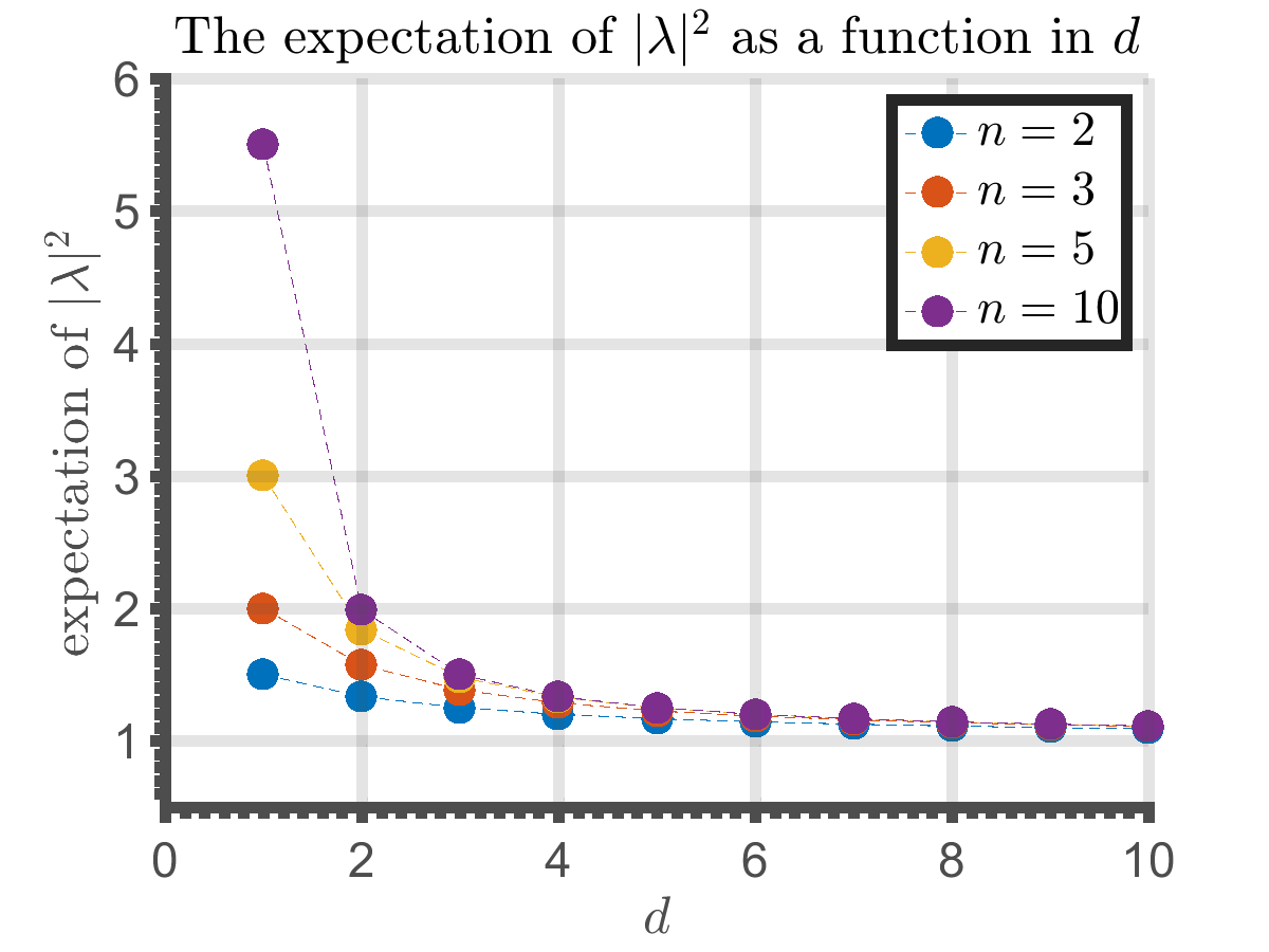
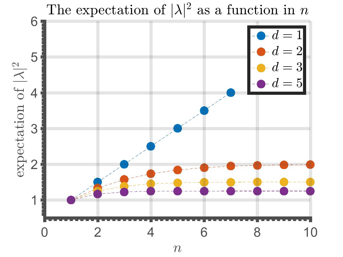
We can compute the expectation of the random variable $\lvert\lambda\rvert^{2}$ ; cf. Figure 1.1.

Corollary 1.3

If $d=1$ , then $\mean\limits_{\lambda\sim\rho^{n,1}}\lvert\lambda\rvert^{2}=\frac{n+1}{2}$ . If $d>1$ , then

\mean\limits_{\lambda\sim\rho^{n,d}}\lvert\lambda\rvert^{2}\ =\ \frac{n-(n+1)d+d^{n+1}}{(d^{n}-1)(d-1)}.

We have $\lim\limits_{d\to\infty}\mean\limits_{\lambda\sim\rho^{n,d}}\lvert\lambda\rvert^{2}=1$ and $\lim\limits_{n\to\infty}\mean\limits_{\lambda\sim\rho^{n,d}}\lvert\lambda\rvert^{2}\ =\ \frac{d}{d-1}$ if $d>1$ . Moreover, for fixed $n$ , the function $d\mapsto\mean\limits_{\lambda\sim\rho^{n,d}}\lvert\lambda\rvert^{2}$ is strictly decreasing. For fixed $d$ , the function $n\mapsto\mean\limits_{\lambda\sim\rho^{n,d}}\lvert\lambda\rvert^{2}$ is strictly increasing.

Refer to caption — Figure 1.1: The left picture shows plots of $d\mapsto\mean\limits_{\lambda\sim\rho^{n,d}}\lvert\lambda\rvert^{2}$ for $n\in\{2,3,5,10\}$ . On the right are plots of $n\mapsto\mean\limits_{\lambda\sim\rho^{n,d}}\lvert\lambda\rvert^{2}$ for $d\in\{1,2,3,5\}$ .

In order to investigate $\rho_{\mathbb{R}}^{n,1}$ for large $n$ , we can normalize $\lvert\lambda\rvert^{2}$ by dividing it by its expectation. We will, however, divide $\lvert\lambda\rvert^{2}$ by $n$ . While for large $n$ this does not make a big difference, the formulas appearing are easier to understand. We will also normalize in the case $d>1$ . So if $d=1$ , we put

\tau:=\frac{\lvert\lambda\rvert^{2}}{n}=\frac{R}{2n},

and if $d>1$ , we put

\tau:=\frac{\lvert\lambda\rvert^{2}}{2\lim\limits_{n\to\infty}\mean\limits_{\lambda\sim\rho^{n,d}}\lvert\lambda\rvert^{2}}=\frac{R(d-1)}{4d}.

(1.2)

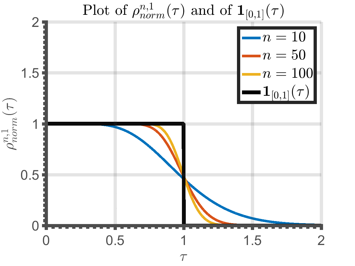
Making a change of variables from $R$ to $\tau$ yields the normalized density, denoted by $\rho^{n,d}_{\textbf{norm}}$ . In [5] Ginibre notes that in the case $d=1$ we have

\lim\limits_{n\to\infty}\rho^{n,1}_{\textbf{norm}}(\tau)=\mathbf{1}_{[0,1]}(\tau):=\begin{cases}1,&\text{ if }0\leq\tau\leq 1\\ 0,&\text{ else}\end{cases}

(1.3)

This means that the distribution of the normalized eigenvalue $\lambda/\sqrt{n}$ converges towards the uniform distribution on the unit ball $\left\{x\in\mathbb{C}\mid\lvert x\rvert\leq 1\right\}$ .

Our third result covers the case $d>1$ .

Theorem 1.4

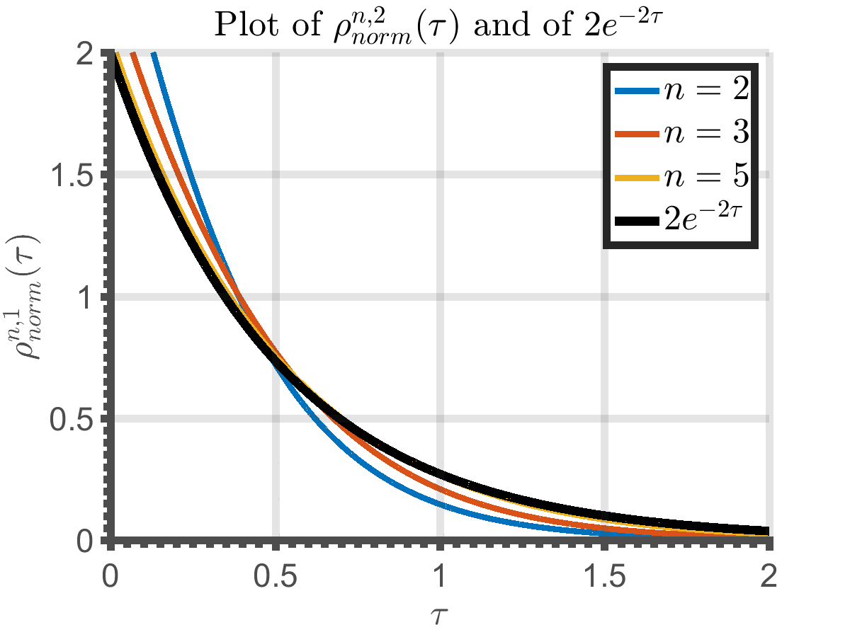
Let $d>1$ be fixed. For any $\tau\geq 0$ we have

\lim_{n\to\infty}\rho^{n,d}_{\textbf{norm}}(\tau)=2\,e^{-2\tau}.

Hence, as $n\to\infty$ , the normalized density $\rho^{n,d}_{\textbf{norm}}(\tau)$ converges towards the exponential distribution with parameter $2$ (cf. Figure 1.2).

1.1 Relation to prior work

Our definition of eigenpairs is inspired by the following definition of E-eigenvalues of tensors and supermatrices given by Qi in [13, sec. 2-3] and [12, sec. 1].

Let $\Phi$ be a multilinear map $(\mathbb{R}^{n})^{d}\to\mathbb{R}^{n}$ , that is represented by the real supermatrix $A=(A_{j,i_{1}\ldots i_{d}})$ . For $v\in\mathbb{R}^{n}$ , Qi puts $A\,v^{d}:=A(v,\ldots,v)$ (see [13, sec. 3, eq. (7)]) and then defines $\lambda\in\mathbb{C}$ to be an E-eigenvalue of $A$ if there exists $v\in\mathbb{C}^{n}$ such that $A\,v^{d}=\lambda v$ and $v^{T}v=1$ . This definition of eigenvalue is independent of the change of orthonormal coordinates. Therefore, $\lambda$ can be regarded as an eigenvalue of $\Phi$ itself. Although assuming $\Phi$ over the reals, Qi allows the eigenvalue to be complex. If the eigenvalue $\lambda$ is real, he calls it a Z-eigenvalue.

In [4] Cartwright and Sturmfels relax the definition of Qi by considering order- $(d+1)$ tensors/supermatrices over the complex numbers $\mathbb{C}$ . They define a pair $(v,\lambda)\in(\mathbb{C}^{n}\backslash\left\{0\right\})\times\penalty\ \mathbb{C}$ to be an eigenpair of $A$ , if

A\,v^{d}=\lambda v.

(1.4)

Observe that Qi’s condition $v^{T}v=1$ implies that $v\neq 0$ , while Sturmfels and Cartwright require the eigenpair to be an element in $(\mathbb{C}\backslash\left\{0\right\})\times\mathbb{C}$ . In reference to Qi they call an eigenpair $(v,\lambda)$ satisfying $v^{T}v=1$ normalized, whereas we call an eigenpair $(v,\lambda)$ normalized, if it satisfies $v^{T}\overline{v}=1$ . In fact, $A\,v^{d}$ is a system of homogeneous polynomials over $\mathbb{C}$ in the entries of $v$ . So 1.4 coincides with our definition.

Another approach to define eigenpairs of homogeneous polynomial systems is given by Lim [10] in his variational approach, which is as follows.

We denote by $\lVert\,\rVert_{k}$ the $\mathcal{L}_{k}$ -norm on $\mathbb{R}^{n}$ for $k>1$ . Suppose that $F(X)$ is a real homogeneous polynomial in $n$ variables $X=(X_{1},\ldots,X_{n})$ of degree $d+1$ . In order to optimize $F$ on the $\mathcal{L}_{k}$ -sphere $\left\{\lVert x\rVert_{k}=1\right\}$ , one can consider the Langrangian of the multilinear Rayleigh quotient $F(X)/\lVert X\rVert_{k}^{d+1}$ , that is $L(X,\Lambda):=F(X)-(d+1)^{-1}\Lambda\,(\lVert X\rVert_{k}^{d+1}-1),$ where $\Lambda$ is an auxiliary variable. Then the equation $\nabla L=0$ gives

\nabla F(X)=\Lambda\,\begin{pmatrix}\mathrm{sgn}(X_{1})^{k}\,X_{1}^{k-1}\\ \vdots\\ \mathrm{sgn}(X_{n})^{k}\,X_{n}^{k-1}\end{pmatrix},\quad\lVert X\rVert_{k}=1.

(1.5)

Note that $\nabla F(X)$ is a system of homogeneous polynomials of degree $d$ . If the pair $(v,\lambda)\in\{\lVert v\rVert_{k}=1\}\times\mathbb{R}$ is a solution of equation 1.5, Lim calls $v$ an $\mathcal{L}^{k}$ -eigenvector and $\lambda$ an $\mathcal{L}^{k}$ -eigenvalue of the system $\nabla F$ . In particular, if $k=2$ , the $\mathcal{L}_{2}$ -eigenvalues $(v,\lambda)\in\{\lVert v\rVert_{2}=1\}\times\mathbb{R}$ satisfy

\nabla F(v)=\lambda\,v,\quad\lVert v\rVert_{2}=1.

If we relax the definition of $\mathcal{L}_{2}$ -eigenvalues by allowing $(v,\lambda)$ to be complex, the pair $(v,\lambda)$ is an eigenpair of the system $\nabla F(X)$ in our sense.

The organization of the paper is as follows. After some preliminaries presented in the next section, we establish in Section 3 the geometric framework for the eigenpair problem. Our concepts and notations are close to the ones from [3, sec. 16]. We define a probability distribution on $\left\{(f,v,\lambda)\mid f(v)=\lambda v\right\}$ , the solution manifold. The pushforward measure of this distribution with respect to the projection onto the space of eigenvalues is precisely $\rho^{n,d}$ . Finally, we prove the stated results in Section 4.

Acknowledgements The basis of this work was laid during the program "Algorithms and Complexity in Algebraic Geometry" at the Simons Institute for the Theory of Computing. We are grateful for the Simons Institute for the stimulating environment and the financial support.

2 Preliminaries

2.1 Differential geometry

We denote by $\langle x,y\rangle:=x^{T}\overline{y}$ the standard hermitian inner product on $\mathbb{C}^{n}$ . Furthermore, we set $\lVert x\rVert:=\sqrt{\langle x,x\rangle}$ and $\mathbb{S}(\mathbb{C}^{n}):=\big\{x\in\mathbb{C}^{n}\mid\lVert x\rVert=1\big\}$ . Given some $x\in\mathbb{C}^{n}\backslash\left\{0\right\}$ we denote by $T_{x}:=\big\{y\in\mathbb{C}^{n}\mid\langle x,y\rangle=0\big\}$ the orthogonal complement of $x$ in $\mathbb{C}^{n}$ .

If $M$ is a differentiable manifold and $x\in M$ we denote by $T_{x}M$ the tangent space of $M$ at $x$ .

Lemma 2.1

Let $v\in\mathbb{S}(\mathbb{C}^{n})$ . Then $T_{v}\mathbb{S}(\mathbb{C}^{n})=\big\{a\in\mathbb{C}^{n}\mid\Re\langle a,v\rangle=0\big\}=T_{v}\oplus\mathbb{R}iv$ and this composition is orthogonal with respect to inner product on $T_{v}\mathbb{S}(\mathbb{C}^{n})$ , that is induced from $\langle\>,\rangle$ .

Proof

See [3, Equation (14.11)] and [3, Lemma 14.9]. _■

If $M$ and $N$ are differentiable manifolds and $F\colon M\to N$ is differentiable, we denote by $DF(x):T_{x}M\to T_{F(x)}N$ its derivative at $x\in M$ and by $NJ(F)(x)$ its normal jacobian at $x$ .

For more details on normal jacobians and the coarea formula we refer to [3, sec. 17.3].

Theorem 2.2 (Coarea formula)

Suppose that $M,N$ are Riemannian manifolds of dimensions $m,n$ , respectively. Let $\Psi:M\to N$ be a surjective smooth map. Then we have for any function $\chi:M\to\mathbb{R}$ that is integrable with respect to the volume measure of $M$ that

\int_{M}\chi\mathrm{d}M=\int_{y\in N}\left[\int_{\Psi^{-1}(y)}\frac{\chi}{NJ(\Psi)}\mathrm{d}\Psi^{-1}(y)\right]\mathrm{d}N.

Let $E_{1},E_{2}$ be finite dimensional complex vector spaces with hermitian inner product, such that $\dim_{\mathbb{C}}E_{1}\geq\dim_{\mathbb{C}}E_{2}$ . Assume that we have a surjective linear map $\phi:E_{1}\to E_{2}$ (think of $\phi$ as a derivative and $E_{1},E_{2}$ being tangent spaces). Let $\Gamma(\phi):=\left\{(x,\phi(x))\in E_{1}\times E_{2}\right\}$ be the graph of $\phi$ . Then $\Gamma(\phi)$ is a linear space and the projections $p_{1}:\Gamma(\phi)\to E_{1}$ and $p_{2}:\Gamma(\phi)\to E_{2}$ are linear maps.

The following result is Lemma 3 in [2, sec. 13.2], combined with the comment in Theorem 5 in [2, sec. 13.2].

Lemma 2.3

Let $W$ be the orthogonal complement of $\ker p_{2}$ . Then we have

\frac{\lvert\det(p_{1})\rvert}{\lvert\det(p_{2}|_{W})\rvert}=\lvert\det(\phi\phi^{*})\rvert^{-1}.

2.2 Expectation of the truncated geometric distribution

The geometric distribution with parameter $p$ truncated at $n\geq 1$ is defined to be the distribution of a geometrically distributed random variable $X$ with parameter $p$ under the condition that $X\leq n$ . Its density is

\Prob\limits_{X\sim\mathrm{Geo}(p)}\left\{X=k\mid X\leq n\right\}=\frac{\Prob\limits_{X\sim\mathrm{Geo}(p)}\left\{X=k\right\}}{\Prob\limits_{X\sim\mathrm{Geo}(p)}\left\{X\leq n\right\}}=\frac{q^{k-1}(1-q)}{1-q^{n}},

(2.1)

where $q:=1-p$ and $k\in\left\{1,\ldots,n\right\}$ .

Lemma 2.4

Let $n\geq 1$ and $0\leq q<1$ . Then

\mean\limits_{X\sim\mathrm{Geo}(1-q)}[X\mid X\leq n]=\frac{nq^{n+1}-(n+1)q^{n}+1}{(1-q^{n})(1-q)}.

Proof

We have $\Prob\limits_{X\sim\mathrm{Geo}(1-q)}\left\{X=k\mid X\leq n\right\}=\frac{q^{k-1}(1-q)}{1-q^{n}}$ , $k\in\left\{1,\ldots,n\right\}$ . This implies

\mean\limits_{X\sim\mathrm{Geo}(1-q)}[X\mid X\leq n]=\frac{1-q}{1-q^{n}}\,\sum_{k=1}^{n}kq^{k-1}.

Observe, that $\sum_{k=1}^{n}kq^{k-1}$ is the derivative of $\frac{1-Z^{n+1}}{1-Z}$ at $Z=q$ and that

\displaystyle\frac{\mathrm{d}\;}{\mathrm{d}Z}\left(\frac{1-Z^{n+1}}{1-Z}\right)=\frac{nZ^{n+1}-(n+1)Z^{n}+1}{(1-Z)^{2}}

Hence the claim. _■

2.3 The expected characteristic polynomial of a random matrix

We say that a random variable $z$ on $\mathbb{C}$ is standard normal distributed if both real and imaginary part of $z$ are i.i.d centered normal distributed random variables with variance $\sigma^{2}=\frac{1}{2}$ . The corresponding density is

\displaystyle\varphi(z):=\frac{1}{\pi}\,\exp\left(-\lvert z\rvert^{2}\right),

and we write $z\sim N(0,\frac{1}{2})$ for this distribution. The reason why we have put $\sigma^{2}=\frac{1}{2}$ is that for a gaussian random variable $z\sim N(0,\frac{1}{2})$ on $\mathbb{C}$ we have

\mean\limits_{z\sim N(0,\frac{1}{2})}\lvert z\rvert^{2}=1.

(2.2)

Suppose that $E$ is a finite dimensional complex vector space with hermitian inner product and let $k:=\dim_{\mathbb{C}}E$ . We define the standard normal density on the space $E$ as

\varphi_{E}(z):=\frac{1}{\pi^{k}}\,\exp\left(-\lVert z\rVert^{2}\right).

(2.3)

it is clear from the context which space is meant, we omit the subscript $E$ . Let $I_{n}$ be the $n\times n$ identity matrix. If a complex matrix $A\in\mathbb{C}^{n\times n}$ is distributed with density $\varphi_{\mathbb{C}^{n\times n}}$ , we write $A\sim N(0,\frac{1}{2}I_{n})$ .

Recall that the Gamma function is defined by $\Gamma(n):=\int_{t=0}^{\infty}t^{n-1}e^{-t}\mathrm{d}t$ for a positive real number $n>0$ . It is well known that $\Gamma(n)=(n-1)!$ if $n$ is a positive integer. The upper incomplete Gamma function is defined as

\Gamma(n,x):=\int_{t=x}^{\infty}t^{n-1}e^{-t}\mathrm{d}t,

where $x\geq 0$ .

Lemma 2.5

1.

Let $x\geq 0$ and $n\geq 1$ . Then $\Gamma(n,x)=(n-1)!\,e^{-x}\sum\limits_{k=0}^{n-1}\frac{x^{k}}{k!}$ .
2.

We have $\mean\limits_{A\sim N\left(0,\frac{1}{2}I_{n}\right)}\lvert\det(A)\rvert^{2}=n!=\Gamma(n-1).$
3.

For $I\subset[n]:=\left\{1,\ldots,n\right\}$ we define $A_{I}\in\mathbb{C}^{\lvert I\rvert\times\lvert I\rvert}$ to be the submatrix of $A\in\mathbb{C}^{n\times n}$ indexed by $I$ . Then for any $t\in\mathbb{C}$ we have that $\det\left(A+tI_{n}\right)=\sum_{I\subset[n]}t^{n-\lvert I\rvert}\det A_{I}.$

Proof

The first assertion is from [6, p. 949], the second is [3, Lemma 4.12], and the third assertion is a well known fact, cf. [8, Theorem 1.2.12]. _■

Proposition 2.6

We have for $A\in\mathbb{C}^{n\times n}$ and $t\in\mathbb{C}$

\mean\limits_{A\sim N\left(0,\frac{1}{2}I_{n}\right)}\lvert\det(A+tI_{n})\rvert^{2}=e^{\lvert t\rvert^{2}}\Gamma\left(n+1,\lvert t\rvert^{2}\right).

Proof

By Lemma 2.5(3), $\det(A+tI_{n\times n})=\sum_{\alpha\in\left\{0,1\right\}^{n}}t^{n-\lvert\alpha\rvert}\det A_{\alpha}$ , hence

\lvert\det(A+tI_{n\times n})\rvert^{2}=\sum_{\alpha,\beta}t^{n-\lvert\alpha\rvert}\,(\overline{t})^{n-\lvert\beta\rvert}\det A_{\alpha}\det\overline{A_{\beta}}.

Due to Lemma 2.5(2), we have $\mean\,[\det A_{\alpha}\det\overline{A_{\beta}}]=\delta_{\alpha,\beta}\,\lvert\alpha\rvert!$ , since we deal with centered distributions. Hence,

\mean\,\lvert\det(A+tI_{n\times n})\rvert^{2}=\sum_{k=0}^{n}\binom{n}{k}\,k!\,\lvert t\rvert^{2(n-k)}=e^{\lvert t\rvert^{2}}\,\Gamma(n+1,\lvert t\rvert^{2});

the last equality by Lemma 2.5(1). _■

3 Geometric framework

3.1 Eigenpairs of homogeneous polynomial systems

Let $n,d\geq 1$ . We denote by $\mathcal{H}_{d}:=\mathcal{H}_{d}(X_{1},\ldots,X_{n})$ the vector space of homogeneous polynomials of degree $d$ in the variables $X_{1},\ldots,X_{n}$ over the complex numbers $\mathbb{C}$ of degree $d$ . The Bombieri-Weyl basis is given by the $e_{\alpha}:=\binom{d}{\alpha}^{\frac{1}{2}}X^{\alpha}$ , $\lvert\alpha\rvert=d$ . We define an inner product on $\mathcal{H}_{d}$ via

\Big\langle\sum\limits_{\alpha}a_{\alpha}e_{\alpha},\sum\limits_{\alpha}b_{\alpha}e_{\alpha}\Big\rangle:=\sum\limits_{\alpha}a_{\alpha}\overline{b_{\alpha}}.

(3.1)

The product 3.1 extends to $(\mathcal{H}_{d})^{n}$ in the following way. Let $f=(f_{1},\ldots,f_{n})$ and $g=(g_{1},\ldots,g_{n})\in(\mathcal{H}_{d})^{n}$ . Then we define $\langle f,g\rangle:=\sum_{i=1}^{n}\langle f_{i},g_{i}\rangle.$ Moreover, for $f\in(\mathcal{H}_{d})^{n}$ we set $\lVert f\rVert:=\sqrt{\langle f,f\rangle}$ .

Remark 3.1

1.

The inner product 3.1 is the unique unitary invariant product on $\mathcal{H}_{d}$ (up to scaling). See [3, Theorem 16.3] and [3, Remark 16.4].
2.

Suppose that $f=(f_{1},\ldots,f_{n})\in(\mathcal{H}_{d})^{n}$ and $f_{i}=\sum_{\alpha}a_{i,\alpha}e_{\alpha}$ , $1\leq i\leq n$ . Let $k:=\dim\mathcal{H}_{d}$ and put $A:=(a_{i,\alpha})\in\mathbb{C}^{n\times k}$ . Then $\lVert f\rVert=\lVert A\rVert_{F}$ , where $\lVert\,\rVert_{F}$ is the Frobenius norm.

For the sake of clarity, we recall the definition of eigenpairs given in the introduction.

Definition 3.2

An eigenpair of $f\in(\mathcal{H}_{d})^{n}$ is a pair $(v,\lambda)\in(\mathbb{C}^{n}\backslash\{0\})\times\mathbb{C}$ such that $f(v)=\lambda v$ . We call $v$ an eigenvector and $\lambda$ an eigenvalue of $f$ . Further, we call eigenpairs $(v,\lambda)$ and $(w,\eta)$ equivalent, $(v,\lambda)\sim(w,\eta)$ , if there exists a nonzero $t\in\mathbb{C}$ such that $(tv,t^{d-1}\lambda)=(w,\eta)$ .

We already noted that the number of equivalence classes of a generic system $f$ equals $D(n,d)=(d^{n}-1)/(d-1)$ if $d>1$ , cf. [4].

3.2 The solution manifold

Let $\mathcal{A}:=\mathbb{C}[X_{1},\ldots,X_{n},\Lambda]$ be the space of polynomials in the $n+1$ variables $X_{1},\ldots,X_{n},\Lambda$ . We consider the map $F:(\mathcal{H}_{d})^{n}\to\mathcal{A}^{n},f\mapsto f(X)-\Lambda X$ . For $f\in(\mathcal{H}_{d})^{n}$ we set $F_{f}:=F(f)$ , such that

F_{f}:\mathbb{C}^{n}\times\mathbb{C}\to\mathbb{C}^{n},\quad(v,\lambda)\mapsto f(v)-\lambda v.

(3.2)

Observe that $F_{f}(X,\Lambda)$ consists of two parts, one homogeneous of degree $d$ and one homogeneous of degree $2$ . Let us denote by $\partial_{X}$ and $\partial_{\Lambda}$ the partial derivatives of $F_{f}(X,\Lambda)$ with respect to $X=(X_{1},\ldots,X_{n})$ and $\Lambda$ , respectively. Then the derivative of $F_{f}$ at $(v,\lambda)$ has the following matrix representation:

\begin{bmatrix}\partial_{X}f-\partial_{X}(\Lambda X),&-\partial_{\Lambda}(\Lambda X)\end{bmatrix}_{(X,\Lambda)=(v,\lambda)}=\begin{bmatrix}\partial_{X}f(v)-\lambda I_{n},&-v\end{bmatrix},

(3.3)

where $I_{n}$ denotes the $n\times n$ -identity matrix.

We adapt the terms “solution manifold” and “well-posed” from [3, sec. 16.2] and tailor them to our (structured) set $\left\{F_{f}\mid f\in(\mathcal{H}_{d})^{n}\right\}$ . Compare [3, Open Problem 15]. We call

\mathcal{V}:=\left\{(f,v,\lambda)\in(\mathcal{H}_{d})^{n}\times\mathbb{S}(\mathbb{C}^{n})\times\mathbb{C}\mid F_{f}(v,\lambda)=0\right\},

the solution manifold and its subset

\mathcal{W}:=\left\{(f,v,\lambda)\in\mathcal{V}\mid\mathrm{rk}\,DF_{f}(v,\lambda)=n\right\}

the manifold of well-posed triples.

The group $\mathcal{U}(n)$ of unitary linear transformations $\mathbb{C}^{n}\to\mathbb{C}^{n}$ acts on $\left(\mathcal{H}_{d}\right)^{n}$ and $\mathcal{V}$ , respectively, via

U.f:=U\circ f\circ U^{-1}\quad\text{and}\quad U.(f,v,\lambda):=(U.f,Uv,\lambda).

(3.4)

We note that $\mathcal{W}$ is invariant under the group action and that $\mathcal{U}(n)$ acts by isometries; see [3, Theorem 16.3].

Lemma 3.3

The solution manifold $\mathcal{V}$ is a connected and smooth submanifold of $(\mathcal{H}_{d})^{n}\times\mathbb{S}(\mathbb{C}^{n})\times\mathbb{C}$ of dimension $\dim_{\mathbb{R}}\mathcal{V}=\dim_{\mathbb{R}}(\mathcal{H}_{d})^{n}+1$ . Moreover, the tangent space of $\mathcal{V}$ at $(f,v,\lambda)$ equals

\left\{(\dot{f},\dot{v},\dot{\lambda})\in(\mathcal{H}_{d})^{n}\times T_{v}\mathbb{S}(\mathbb{C}^{n})\times\mathbb{C}\mid\dot{f}(v)+DF_{f}(v,\lambda)(\dot{v},\dot{\lambda})=0\right\}.

Proof

The map $G:(\mathcal{H}_{d})^{n}\times\mathbb{S}(\mathbb{C}^{n})\times\mathbb{C}\to\mathbb{C}^{n},(f,v,\lambda)\mapsto F_{f}(v,\lambda)$ has $\mathcal{V}$ as its fiber over $0$ . The derivative of $G$ ,

DG(f,v,\lambda):\;(\mathcal{H}_{d})^{n}\times T_{v}\mathbb{S}(\mathbb{C}^{n})\times\mathbb{C}\to\mathbb{C}^{n},\ (\dot{f},\dot{v},\dot{\lambda})\mapsto\dot{f}(v)+DF_{f}(v,\lambda)(\dot{v},\dot{\lambda}),

is clearly surjective. Therefore $0\in\mathbb{C}^{n}$ is a regular value of $G$ and Theorem A.9 in [3] implies the assertion. _■

The following lemma is easily verfied using Euler’s identity for homogeneous functions.

Lemma 3.4

Let $(f,v,\lambda)\in\mathcal{W}$ . Then $\ker DF_{f}(v,\lambda)=\mathbb{C}\,(v,(d-1)\lambda)^{T}$ . In particular, $DF_{f}(v,\lambda)|_{T_{v}\times\mathbb{C}}$ is invertible.

Corollary 3.5

The tangent space $T_{(f,v,\lambda)}\mathcal{V}$ at $(f,v,\lambda)\in\mathcal{W}$ is given by

\Big\{(\dot{f},\dot{v}+riv,\dot{\lambda})\in(\mathcal{H}_{d})^{n}\times(T_{v}\oplus\mathbb{R}iv)\times\mathbb{C}\mid(\dot{v},\dot{\lambda})=-DF_{f}(v,\lambda)|_{T_{v}\times\mathbb{C}}^{-1}\,\dot{f}(v)\Big\}.

Proof

Let $(f,v,\lambda)\in\mathcal{V}$ be fixed. By Lemma 3.3 the tangent space of $\mathcal{V}$ at $(f,v,\lambda)$ equals

\left\{(\dot{f},\dot{w},\dot{\lambda})\in(\mathcal{H}_{d})^{n}\times T_{v}\mathbb{S}(\mathbb{C}^{n})\times\mathbb{C}\mid DF_{f}(v,\lambda)\,(\dot{w},\dot{\lambda})=-\dot{f}(v)\right\}.

From Lemma 2.1 we know that $T_{v}\mathbb{S}(\mathbb{C}^{n})=T_{v}\oplus\mathbb{R}iv$ . Lemma 3.4 tells us that

\ker DF_{f}(v,\lambda)=\mathbb{C}(v,(d-1)\lambda)=\mathbb{R}(v,(d-1)\lambda)\oplus\mathbb{R}i(v,(d-1)\lambda).

Hence, $(T_{v}\mathbb{S}(\mathbb{C}^{n})\times\mathbb{C})\cap\ker DF_{f}(v,\lambda)=\mathbb{R}i(v,(d-1)\lambda)$ . From Lemma 3.4 we know that $DF_{f}(v,\lambda)|_{T_{v}\times\mathbb{C}}$ is invertible. We conclude that if $(\dot{f},\dot{w},\dot{\lambda})\in T_{(f,v,\lambda)}\mathcal{V}$ , then there exist uniquely determined $\dot{v}\in T_{v}$ and $r\in\mathbb{R}$ such that $\dot{w}=\dot{v}+irv$ and $DF_{f}(v,\lambda)(\dot{w},\dot{\lambda})=DF_{f}(v,\lambda)(\dot{v},\dot{\lambda})$ , from which the claim follows. _■

3.3 Projections and normal jacobians

We consider the projections

\pi_{1}\colon\mathcal{V}\to(\mathcal{H}_{d})^{n},(f,v,\lambda)\mapsto f,\quad\pi_{2}\colon\mathcal{V}\to\mathbb{S}(\mathbb{C}^{n})\times\mathbb{C},(f,v,\lambda)\mapsto(v,\lambda).

(3.5)

It is essential that the quotient of the normal jacobians of $\pi_{1}$ and $\pi_{2}$ can be computed in the following way.

Lemma 3.6

For all $(f,v,\lambda)\in\mathcal{W}$ we have

\frac{NJ(\pi_{1})(f,v,\lambda)}{NJ(\pi_{2})(f,v,\lambda)}=\left\lvert\det(DF_{f}(f,v,\lambda)|_{T_{v}\times\mathbb{C}})\right\rvert^{2}.

Proof

Let $\mathcal{U}(n)$ be group of unitary maps $\mathbb{C}^{n}\to\mathbb{C}^{n}$ . Recall from 3.4 that for $U\in\mathcal{U}(n)$ and $(f,v,\lambda)\in\mathcal{V}$ we have put $U.(f,v,\lambda):=(U.f,Uv,\lambda)$ . By definition, the projections $\pi_{1},\pi_{2}$ are $\mathcal{U}(n)$ -equivariant. Hence for any $U\in\mathcal{U}(n)$ we have $NJ(\pi_{i})(f,v,\lambda)=NJ(\pi_{i})(U.(f,v,\lambda))$ , $i=1,2$ . It therefore suffices to show the claim for $v=e_{1}$ , where $e_{1}:=(1,0,\ldots,0)\in\mathbb{C}^{n}$ .

Suppose that $(f,e_{1},\lambda)\in\mathcal{W}$ . The derivatives of $\pi_{1}$ and $\pi_{2}$ are the projections

\begin{array}[]{lll}D\pi_{1}(f,e_{1},\lambda):&T_{(f,e_{1},\lambda)}\mathcal{V}\to(\mathcal{H}_{d})^{n},&(\dot{f},\dot{v},\dot{\lambda})\mapsto\dot{f},\\ D\pi_{2}(f,e_{1},\lambda):&T_{(f,e_{1},\eta)}\mathcal{V}\to T_{e_{1}}\mathbb{S}(\mathbb{C}^{n})\times\mathbb{C},&(\dot{f},\dot{v},\dot{\lambda})\mapsto(\dot{v},\dot{\lambda}).\end{array}

Let us write $\dot{f}=\sum\limits_{\alpha}\dot{f}_{\alpha}X^{\alpha}$ , where for all $\alpha$ we have $\dot{f}_{\alpha}\in\mathbb{C}^{n}$ . Then we obtain $\dot{f}(e_{1})=\dot{f}_{(d,0,\ldots,0)}$ . Hence, $\dot{f}\mapsto\dot{f}(e_{1})$ is an orthogonal projection. We will denote this projection by $\Pi$ . By Lemma 2.1 the projection $\dot{v}+riv\mapsto\dot{v}$ is orthogonal as well. Using Corollary 3.5 it follows that $T_{(f,e_{1},\lambda)}\mathcal{V}$ is the graph of the surjective linear function

-DF_{f}(e_{1},\lambda)|_{T_{e_{1}}\times\mathbb{C}}^{-1}\;\circ\;(\Pi\times 0):\>(\mathcal{H}_{d})^{n}\times\mathbb{R}iv\to T_{e_{1}}\times\mathbb{C}.

Applying Lemma 2.3 yields the claim. _■

3.4 The eigendiscriminant variety

We define the set of ill-posed triples $(f,v,\lambda)$ to be

\Sigma^{\prime}:=\left\{(f,v,\lambda)\in\mathcal{V}\mid\mathrm{rk}\,DF_{f}(v,\lambda)<n\right\}=\mathcal{V}\backslash\mathcal{W}.

(3.6)

Moreover, we denote by $\Sigma$ the Zariski closure of $\overline{\pi_{1}(\Sigma^{\prime})}$ . In reference to [1], we call $\Sigma$ the eigendiscriminant variety.

Remark 3.7

We have $(f,v,\lambda)\in\Sigma^{\prime}$ if and only if $(v,\lambda)$ is not an isolated root of the polynomial $F_{f}$ . Thus, $f\in\pi_{1}(\Sigma^{\prime})$ if and only if $F_{f}$ has a double root or $f$ has infinitely many roots.

Proposition 3.8

1.

We have $f\not\in\Sigma$ , if and only if the number of equivalence classes of $f$ equals $D(n,d)$ .
2.

The set $\Sigma$ is a closed hypersurface of $(\mathcal{H}_{d})^{n}$ of degree at most $n(n-1)d^{n-1}$ .

Proof

For Item 1 use [4, Theorem 1.2]. In [1, Theorem 4.1, Corollary 4.2] it is shown that the eigendiscriminant variety for tensors in $(\mathbb{C}^{n})^{\otimes d}$ is an irreducible hypersurface. We obtain $\Sigma$ by intersecting this with the linear subspace of symmetric tensors and requiring $\|v\|=1$ . The assertion Item 2 follows from the dimension theorem, Bezout’s theorem and the fact that $\Sigma$ is properly contained in $(\mathcal{H}_{d})^{n}$ (see Proposition 3.9 below). _■

In [14] the following explicit element in $(\mathcal{H}_{d})^{n}\backslash\Sigma$ is described ( $d>1$ ).

Proposition 3.9

Let $\phi(X):=\left(X_{1}^{d},X_{2}^{d},\ldots,X_{n}^{d}\right)\in(\mathcal{H}_{d})^{n}$ . Then $\phi\not\in\Sigma$ .

Proof

One has

F_{\phi}(X,\Lambda)=\begin{pmatrix}X_{1}^{d}-\Lambda X_{1}\\ \vdots\\ X_{n}^{d}-\Lambda X_{n}\end{pmatrix}.

We are going to show that $\phi$ has exactly $D(n,d)$ many classes of eigenpairs. Clearly, for any $v\in\mathbb{C}\backslash\left\{0\right\}$ we have $F_{\phi}(v,0)\neq 0$ . Hence, any equivalence class of eigenpairs of $\phi$ contains some representative of the form $(v,1)$ . Let $\zeta$ be a primitive $(d-1)$ -th root of unity and define

M:=\Big\{(\epsilon_{1}\zeta^{i_{1}},\ldots,\epsilon_{n}\zeta^{i_{n}})\mid\epsilon\in\left\{0,1\right\}^{n}\backslash\left\{0\right\},\forall j:1\leq i_{j}\leq d-1\Big\}

Observe that $F_{\phi}(z,1)=(z_{i}^{d}-z_{i})_{i=1}^{n}=0$ , if and only if $z\in M\cup\left\{0\right\}$ . For all $z\in M$ and $t\in\mathbb{C}$ we have $(z,1)\sim(tz,1)$ if and only if $t=\zeta^{i}$ for some $1\leq i\leq d-1$ . Let $\mathfrak{U}:=\langle\zeta\rangle$ denote the cyclic group generated by $\zeta$ . We define a group action of $\mathfrak{U}$ on $M$ via componentwise multiplication. The number of equivalence classes of eigenpairs of $\phi$ then equals the number of $\mathfrak{U}\text{-orbits}$ in $M$ . For $u\in\mathfrak{U}$ put $M^{u}:=\left\{z\in M\mid uz=z\right\}$ . Observe that for $u\neq 1$ we have that $M^{u}=\emptyset$ . Using Burnside’s lemma we obtain

\text{number of }\mathfrak{U}\text{-orbits in }M=\frac{1}{\lvert\mathfrak{U}\rvert}\,\sum_{u\in\mathfrak{U}}\lvert M^{u}\rvert=\frac{1}{\lvert\mathfrak{U}\rvert}\,\lvert M\rvert=\frac{d^{n}-1}{d-1}=D(n,d).

_■

3.5 The standard distribution on the solution manifold

The definition of standard distribution is adapted from [3, eq. (17.19)]. Following 2.3, we say that a random variable $f$ on $(\mathcal{H}_{d})^{n}$ is standard normal distributed, if $f$ has the density

\varphi(f):=\varphi_{(\mathcal{H}_{d})^{n}}(f)=\frac{1}{\pi^{k}}\,\exp\left(-\lVert f\rVert^{2}\right),\quad\text{ where }k=\dim_{\mathbb{C}}(\mathcal{H}_{d})^{n}.

By construction $\varphi(f)$ is invariant under the action of $\mathcal{U}(n)$ .

The following procedure:

1.

choose $f$ according to the standard normal distribution.
2.

choose some normalized eigenpair $(v,\lambda)$ of $f$ uniformly at random.

yields a probability distribution on $\mathcal{V}$ , which we call the standard distribution and denote it by $(f,v,\lambda)\sim{\mathrm{STD}_{\mathcal{V}}}$ . Clearly, the standard distribution is invariant under the action of $\mathcal{U}(n)$ on $\mathcal{V}$ .

Observe that the two steps above are precisely the steps Item 1–Item 3 in the operative description of $\rho^{n,d}$ given in the introduction. This implies that $\rho^{n,d}$ equals the density of the pushforward measure of $\mathrm{STD}_{\mathcal{V}}$ with respect to the projection $\pi_{3}\colon\mathcal{V}\to\mathbb{C},\,(f,v,\lambda)\mapsto\lambda$ .

According to Proposition 3.8, the fiber

V(f):=\left\{(v,\lambda)\in\mathbb{S}(\mathbb{C}^{n})\times\mathbb{C}\mid(f,v,\lambda)\in\mathcal{V}\right\}=\pi_{2}(\pi_{1}^{-1}(f))

over $f\not\in\Sigma$ consists of $D=D(n,d)$ disjoint circles, each of them having volume $2\pi$ . Hence the density of the uniform distribution on $V(f)$ equals $(2\pi D)^{-1}$ . As in [3, Lemma 17.18], one can now show that the density of the standard distribution is given by

\rho_{\mathrm{STD}_{\mathcal{V}}}(f,v,\lambda)=\frac{1}{2\pi D(n,d)}\,NJ(\pi_{1})(f,v,\lambda)\,\varphi(f),

(3.7)

where $\pi_{1}:\mathcal{V}\to(\mathcal{H}_{d})^{n}$ is the projection from (3.5).

We denote by

V(v,\lambda):=\left\{f\in(\mathcal{H}_{d})^{n}\mid(f,v,\lambda)\in\mathcal{V}\right\}=\pi_{1}(\pi_{2}^{-1}(v,\lambda))

the fiber of $\pi_{2}$ over $(v,\lambda)\in\mathbb{S}(\mathbb{C}^{n})\times\mathbb{C}$ .

Lemma 3.10

Let $\theta:\mathcal{V}\to\mathbb{R}$ be an integrable map that is invariant under the group action from 3.4 and $e_{1}:=(1,0,\ldots,0)\in\mathbb{S}(\mathbb{C}^{n})$ . Then

\int_{(f,v,\lambda)\in\mathcal{V}}\theta(f,v,\lambda)\,\rho_{\mathrm{STD}_{\mathcal{V}}}(f,v,\lambda)\mathrm{d}\mathcal{V}=\frac{\pi^{n-1}}{\Gamma(n)D(n,d)}\int\limits_{\lambda\in\mathbb{C}}E(\lambda)\,\mathrm{d}\mathbb{C}.

where

E(\lambda)=\int\limits_{f\in V(e_{1},\lambda)}\left\lvert\det DF_{f}(e_{1},\lambda)\right\rvert^{2}\,\theta(f,e_{1},\lambda)\,\varphi_{V(e_{1},\lambda)}(f)\;\mathrm{d}V(e_{1},\lambda).

Proof

Using the coarea formula, we obtain

		$\displaystyle\int_{(f,v,\lambda)\in\mathcal{V}}\theta(f,v,\lambda)\,\rho_{\mathrm{STD}_{\mathcal{V}}}(f,v,\lambda)\mathrm{d}\mathcal{V}$
	$\displaystyle=$	$\displaystyle\int_{(v,\lambda)\in\mathbb{S}(\mathbb{C}^{n})\times\mathbb{C}}\left[\int_{f\in V(v,\lambda)}\frac{\theta(f,v,\lambda)\,\rho_{\mathrm{STD}_{\mathcal{V}}}(f,v,\lambda)}{NJ(\pi_{2})(f,v,\lambda)}\mathrm{d}V(v,\lambda)\right]\mathrm{d}(\mathbb{S}(\mathbb{C}^{n})\times\mathbb{C})$

By the definition of $\rho_{\mathrm{STD}_{\mathcal{V}}}$ , Lemma 3.6, and the unitary invariance of $\theta$ we have that

	$\displaystyle\int_{f\in V(v,\lambda)}\frac{\theta(f,v,\lambda)}{NJ(\pi_{2})(f,v,\lambda)}\,\rho_{\mathrm{STD}_{\mathcal{V}}}\;\mathrm{d}V(v,\lambda)$
$\displaystyle=$	$\displaystyle\;\frac{1}{2\pi D}\int_{f\in V(v,\lambda)}\lvert\det DF_{f}(v,\lambda)\|_{T_{v}\times\mathbb{C}}\rvert^{2}\,\theta(f,v,\lambda)\,\varphi(f)\;\mathrm{d}V(v,\lambda)$
$\displaystyle=$	$\displaystyle\;\frac{1}{2\pi D}\int_{f\in V(e_{1},\lambda)}\lvert\det DF_{f}(e_{1},\lambda)\|_{T_{e_{1}}\times\mathbb{C}}\rvert^{2}\,\theta(f,e_{1},\lambda)\,\varphi(f)\;\mathrm{d}V(e_{1},\lambda)$
$\displaystyle=$	$\displaystyle\;\frac{E(\lambda)}{2\pi D}.$	(3.8)

Observe that the integral 3.8 does not depend on $v$ anymore. The claim follows by using $\int 1\mathrm{d}\mathbb{S}(\mathbb{C}^{n})=\frac{2\pi^{n}}{\Gamma(n)}$ _■

4 Proofs

We are now ready to prove Theorem 1.1.

Proposition 4.1

The pushforward density of ${\mathrm{STD}_{\mathcal{V}}}$ with respect to $\pi_{3}$ is

\displaystyle\rho^{n,d}(\lambda)

\displaystyle=\frac{d^{n-1}\,e^{-\lvert\lambda\rvert^{2}\left(1-\frac{1}{d}\right)}}{\pi D(n,d)}\,\frac{\Gamma\left(n,\frac{\lvert\lambda\rvert^{2}}{d}\right)}{\Gamma(n)}=\frac{d^{n-1}\,e^{-\lvert\lambda\rvert^{2}}}{\pi D(n,d)}\,\sum_{k=0}^{n-1}\frac{1}{k!}\,\left(\frac{\lvert\lambda\rvert^{2}}{d}\right)^{k}

Proof

Before we start, we remark that Lemma 2.5 justifies the right equality. By Lemma 3.10, the pushforward distribution $\rho^{n,d}(\lambda)$ is obtained by computing

\frac{\pi^{n-1}}{\Gamma(n)D(n,d)}\int_{f\in V(e_{1},\lambda)}\left\lvert\det DF_{f}(e_{1},\lambda)|_{T_{e_{1}}\times\mathbb{C}}\right\rvert^{2}\varphi_{V(e_{1},\lambda)}(f)\mathrm{d}V(e_{1},\lambda)

(4.1)

The case $n=1$ is an easy exercise. So let us assume that $n>1$ . Observe that $V(e_{1},\lambda)$ is the affine space

V(e_{1},\lambda)=\lambda X_{1}^{d}e_{1}+\Big\{g\in(\mathcal{H}_{d})^{n}\mid g(e_{1})=0\Big\}.

Let $R:=\Big\{h\in(\mathcal{H}_{d})^{n}\mid h(e_{1})=0,Dh(e_{1})=0\Big\}$ . By [3, equation (16.10)], for any $f\in V(e_{1},\lambda)$ , there exist uniquely determined $h\in R$ and $M\in\mathbb{C}^{n\times(n-1)}$ such that we can orthogonally decompose $f$ as

f=\lambda X_{1}^{d}e_{1}+X_{1}^{d-1}\sqrt{d}M\,X^{\prime}+h,

(4.2)

where $X^{\prime}=(X_{2},\ldots,X_{n})^{T}$ . We have that

\partial_{X}f(e_{1},\lambda)=\begin{bmatrix}\partial_{X_{1}}f(e_{1},\lambda),&\partial_{X^{\prime}}f(e_{1},\lambda)\end{bmatrix}=\begin{bmatrix}d\lambda e_{1},&\sqrt{d}M\end{bmatrix}\in\mathbb{C}^{n\times n}

(4.3)

Let $a\in\mathbb{C}^{1\times(n-1)}$ be the first row of $M$ and $A\in\mathbb{C}^{(n-1)\times(n-1)}$ be the matrix that is obtained by removing the first row of $M$ . By 3.3 and 4.3 the derivative of $F_{f}$ at $(e_{1},\lambda)$ has the matrix representation

\begin{bmatrix}\partial_{X}f(e_{1},\lambda)-\lambda I_{n},&-e_{1}\end{bmatrix}=\begin{bmatrix}(d-1)\lambda&\sqrt{d}\,a&-1\\ 0&\sqrt{d}A-\lambda I_{n-1}&0\end{bmatrix}\in\mathbb{C}^{n\times(n+1)}.

This implies $\det DF_{f}(e_{1},\lambda)|_{T_{e_{1}}\times\mathbb{C}}=-\det\;(\sqrt{d}A-\lambda I_{n-1}).$

The summands in 4.2 are pairwise orthogonal. From this we get that $\lVert f\rVert^{2}=\lvert\lambda\rvert^{2}+\lVert M\rVert_{F}^{2}+\penalty\ \lVert h\rVert^{2}$ , which implies that

\varphi_{V(e_{1},\lambda)}(f)=\frac{1}{\pi^{n}}\,e^{-\lvert\lambda\rvert^{2}}\,\varphi_{\mathbb{C}^{(n-1)\times(n-1)}}(A)\,\varphi_{\mathbb{C}^{n}}(a)\,\varphi_{R}(h).

Integrating over $a$ and $h$ in 4.1 therefore yields

		$\displaystyle\int_{f\in V(e_{1},\lambda)}\left\lvert\det DF_{f}(e_{1},\lambda)\|_{T_{e_{1}}\times\mathbb{C}}\right\rvert^{2}\varphi_{V(e_{1},\lambda)}(f)\mathrm{d}V(e_{1},\lambda)$
	$\displaystyle=\>$	$\displaystyle\frac{e^{-\lvert\lambda\rvert^{2}}}{\pi^{n}}\,\mean\limits_{A\sim N(0,\frac{1}{2}I_{n-1})}\left\lvert\det\left(\sqrt{d}\,A-\lambda I_{n-1}\right)\right\rvert^{2}$
	$\displaystyle=\>$	$\displaystyle\frac{d^{n-1}e^{-\lvert\lambda\rvert^{2}}}{\pi^{n}}\,\mean\limits_{A\sim N(0,\frac{1}{2}I_{n-1})}\left\lvert\det\left(A-\frac{\lambda}{\sqrt{d}}I_{n-1}\right)\right\rvert^{2}$
	$\displaystyle=\>$	$\displaystyle\frac{d^{n-1}}{\pi^{n}}\,e^{-\lvert\lambda\rvert^{2}(1-\frac{1}{d})}\,\Gamma\left(n,\frac{\lvert\lambda\rvert^{2}}{d}\right);$

the last line by Proposition 2.6. Plugging this into 4.1 the claim follows. _■

Proof (Proof of Theorem 1.1)

Proposition 4.1 shows that the distribution of the eigenvalue $\lambda$ only depends on $\lvert\lambda\rvert$ . As in 1.1 we put $r:=\lvert\lambda\rvert$ and $R:=2r^{2}$ . Making a change of variables, we obtain the density $\rho^{n,d}_{\mathbb{R}}(R):=\frac{\pi}{2}\,\rho^{n,d}(r)$ . From Proposition 4.1 we obtain

\rho^{n,d}_{\mathbb{R}}(R)=\frac{d^{n-1}}{2D(n,d)}\,e^{-\frac{R}{2}}\,\sum_{k=0}^{n-1}\frac{1}{k!}\left(\frac{R}{2d}\right)^{k}.

(4.4)

If $d=1$ , 4.4 becomes

\rho^{n,1}_{\mathbb{R}}(R)=\frac{1}{n}\,\sum\limits_{k=0}^{n-1}\frac{e^{-\frac{R}{2}}R^{k}}{2^{k+1}k!}=\frac{1}{n}\,\sum\limits_{k=1}^{n}\frac{e^{-\frac{R}{2}}R^{k-1}}{2^{k}(k-1)!}.

For any $k$ we have that $e^{-\frac{R}{2}}\,R^{k-1}/(2^{k}(k-1)!)$ is the density of a chi-square distributed random variable with $2k$ degrees of freedom, which proves the assertion in this case.

If $d>1$ , put $q:=\frac{1}{d}$ , such that $D(n,d)=(1-q^{n})/(q^{n-1}(1-q))$ . Then 4.4 becomes

\rho^{n,d}_{\mathbb{R}}(R)=\sum\limits_{k=0}^{n-1}\frac{e^{-\frac{R}{2}}\,R^{k}}{2^{k+1}k!}\,\frac{(1-q)q^{k}}{1-q^{n}}=\sum\limits_{k=1}^{n}\frac{e^{-\frac{R}{2}}\,R^{k-1}}{2^{k}(k-1)!}\,\frac{(1-q)q^{k-1}}{1-q^{n}}.

Using that $\prob\limits_{X\sim\mathrm{Geo}(1-q)}\left\{X=k\mid X\leq n\right\}=q^{k-1}(1-q)/(1-q^{n})$ , see 2.1, finishes the proof. _■

To prove Corollary 1.3 we will need the following lemma.

Lemma 4.2

Let $n\geq 1$ .

1.

If $d=1$ , then $\mean\limits_{\lambda\sim\rho^{n,1}}\lvert\lambda\rvert^{2}=\mean\limits_{X\sim\mathrm{Unif}(\left\{1,\ldots,n\right\})}[X],$
2.

If $d>1$ , then $\mean\limits_{\lambda\sim\rho^{n,d}}\lvert\lambda\rvert^{2}=\mean\limits_{X\sim\mathrm{Geo}(1-\frac{1}{d})}[X\mid X\leq n].$

Proof

We prove the claim for $d>1$ . (The case $d=1$ is proven similarly.) If $R=2\lvert\lambda\rvert^{2}$ , then $\mean\limits_{\lambda\sim\rho^{n,d}}[\lvert\lambda\rvert^{2}]=\frac{1}{2}\mean[R]$ . From Theorem 1.1 we get

	$\displaystyle\mean[R]$	$\displaystyle=\int_{R=0}^{\infty}R\,\rho^{n,d}_{\mathbb{R}}(R)\mathrm{d}R$
		$\displaystyle=\sum_{k=1}^{n}\prob\limits_{X\sim\mathrm{Geo}(1-\frac{1}{d})}\left\{X=k\mid X\leq n\right\}\,\int_{R=0}^{n}R\,\chi^{2}_{2k}(R)\mathrm{d}R.$
		$\displaystyle=\sum_{k=1}^{n}\prob\limits_{X\sim\mathrm{Geo}(1-\frac{1}{d})}\left\{X=k\mid X\leq n\right\}\,2k\;=\;2\mean\limits_{X\sim\mathrm{Geo}(1-\frac{1}{d})}[X\mid X\leq n],$

where we have used that a $\chi_{2k}^{2}$ -distributed random variable with $2k$ degrees of freedom has the expectation $2k$ . _■

Proof (Proof of Corollary 1.3)

If $d=1$ , from Lemma 4.2 we immediately get $\mean\limits_{\lambda\sim\rho^{n,1}}\lvert\lambda\rvert^{2}=\frac{n+1}{2}.$

If $d>1$ , by Lemma 4.2, we have that $\mean\limits_{\lambda\sim\rho^{n,d}}\lvert\lambda\rvert^{2}=\mean\limits_{X\sim\mathrm{Geo}(1-\frac{1}{d})}[X\mid X\leq n].$ Therefore, Lemma 2.4 with $q:=\frac{1}{d}$ implies

\mean\limits_{\lambda\sim\rho^{n,d}}\lvert\lambda\rvert^{2}=\frac{n-(n+1)d+d^{n+1}}{(d^{n}-1)(d-1)}

as claimed. For fixed $n$ we obtain

\lim\limits_{d\to 1}\frac{n-(n+1)d+d^{n+1}}{(d^{n}-1)(d-1)}=\frac{n+1}{2}

by using de l’Hopital’s rule twice. Therefore, the map

\mathbb{R}_{\geq 1}\to\mathbb{R},\quad d\mapsto\begin{cases}\frac{n+1}{2},&\text{if }d=1\\ \frac{n-(n+1)d+d^{n+1}}{(d^{n}-1)\,(d-1)},&\text{if }d>1\end{cases}.

is continous and differentiable on $\mathbb{R}_{>1}$ . One checks that its derivative on $\mathbb{R}_{>1}$ is negative. Hence, for fixed $n$ , we see that $d\mapsto\mean\limits_{\lambda\sim\rho^{n,d}}[\lvert\lambda\rvert^{2}]$ is strictly decreasing. In the same way we can prove that, if $d$ is fixed, $n\mapsto\mean\limits_{\lambda\sim\rho^{n,d}}[\lvert\lambda\rvert^{2}]$ is strictly increasing. Further,

\lim\limits_{d\to\infty}\frac{n-(n+1)d+d^{n+1}}{(d^{n}-1)\,(d-1)}=\lim\limits_{q\to 0}\frac{nq^{n+1}-(n+1)q^{n}+1}{(1-q^{n})\,(1-q)}=1

If $d>1$ , we have

\lim\limits_{n\to\infty}\mean\limits_{\lambda\sim\rho^{n,d}}[\lvert\lambda\rvert^{2}]=\lim\limits_{n\to\infty}\frac{nq^{n+1}-(n+1)q^{n}+1}{(1-q^{n})\,(1-q)}=\frac{1}{1-q},

where again $q=\frac{1}{d}$ . _■

Proof (Proof of Theorem 1.4)

Let $d>1$ . Recall from 1.2 that we have put $\tau=\frac{R(d-1)}{4d}$ and that we denote the density of $\tau$ by $\rho^{n,d}_{\textbf{norm}}$ . Using Theorem 1.1 we get

\rho^{n,d}_{\textbf{norm}}(\tau)=\frac{4d}{d-1}\,\rho^{n,d}_{\mathbb{R}}\left(\frac{4d\tau}{d-1}\right)=\frac{2d^{n}}{d^{n}-1}\,e^{\frac{-2d\tau}{d-1}}\,\sum_{k=0}^{n-1}\frac{1}{k!}\left(\frac{2\tau}{d-1}\right)^{k}.

Again putting $q=\frac{1}{d}$ we obtain

\rho^{n,d}_{\textbf{norm}}(\tau)=\frac{2}{1-q^{n}}\,e^{\frac{-2\tau}{1-q}}\,\sum_{k=0}^{n-1}\frac{1}{k!}\left(\frac{2q\tau}{1-q}\right)^{k}.

Since $0<q<1$ , we have $\lim\limits_{n\to\infty}q^{n}=0$ . Hence,

\lim_{n\to\infty}\rho^{n,d}_{\textbf{norm}}(\tau)=2\,e^{\frac{-2\tau}{1-q}}\,\sum_{k=0}^{\infty}\frac{1}{k!}\left(\frac{2q\tau}{1-q}\right)^{k}=2\,e^{-2\tau},

which finishes the proof. _■

References

[1] H. Abo, A. Seigal, and B. Sturmfels. Eigenconfigurations of Tensors. ArXiv e-prints, May 2015.
[2] Lenore Blum, Felipe Cucker, Michael Shub, and Steve Smale. Complexity and real computation. Springer-Verlag, New York, 1998.
[3] Peter Bürgisser and Felipe Cucker. Condition, volume 349 of Grundlehren der Mathematischen Wissenschaften. Springer, Heidelberg, 2013.
[4] Dustin Cartwright and Bernd Sturmfels. The number of eigenvalues of a tensor. Linear Algebra Appl., 438(2):942–952, 2013.
[5] Jean Ginibre. Statistical ensembles of complex, quaternion, and real matrices. J. Mathematical Phys., 6:440–449, 1965.
[6] I. S. Gradshteyn and I. M. Ryzhik. Table of integrals, series, and products. Elsevier/Academic Press, Amsterdam, eighth edition, 2015.
[7] Christopher J. Hillar and Lek-Heng Lim. Most tensor problems are NP-hard. J. ACM, 60(6):Art. 45, 39, 2013.
[8] R.A. Horn and C.R. Johnson. Matrix analysis, volume 349. Cambridge University Press, Cambridge, 1992.
[9] Guoyin Li, Liqun Qi, and Gaohang Yu. The $Z$ -eigenvalues of a symmetric tensor and its application to spectral hypergraph theory. Numer. Linear Algebra Appl., 20(6):1001–1029, 2013.
[10] L.-H. Lim. Singular Values and Eigenvalues of Tensors: A Variational Approach. ArXiv Mathematics e-print 060764, July 2006.
[11] L.-H. Lim, M. K. Ng, and L. Qi. The spectral theory of tensors and its applications. Numer. Lin. Algebra Appl., 20(6):889–890, 2013.
[12] Liqun Qi. Eigenvalues of a real supersymmetric tensor. J. Symbolic Comput., 40(6):1302–1324, 2005.
[13] Liqun Qi. Eigenvalues and invariants of tensors. J. Math. Anal. Appl., 325(2):1363–1377, 2007.
[14] E. Robeva. Orthogonal Decomposition of Symmetric Tensors. ArXiv e-print 1409.6685, September 2014.

Plots: MATLAB R2015b