跳到论文正文
W Papers独立论文阅读器 arXiv:1507.02482 论文正文 计算阅读时间 · 0%
引用这篇论文根据当前论文元数据生成,正式投稿前建议核对。


License: arXiv.org perpetual non-exclusive license
arXiv:1507.02482v4 [cs.DS] 21 Aug 2017

Differentially Private Ordinary Least Squares

Or Sheffet Affiliation: Computing Science Dept., University of Alberta, Edmonton AB, Canada. This work was done when the author was at Harvard University, supported by NSF grant CNS-123723 Correspondence to: osheffet@ualberta.ca
Abstract

Linear regression is one of the most prevalent techniques in machine learning; however, it is also common to use linear regression for its explanatory capabilities rather than label prediction. Ordinary Least Squares (OLS) is often used in statistics to establish a correlation between an attribute (e.g. gender) and a label (e.g. income) in the presence of other (potentially correlated) features. OLS assumes a particular model that randomly generates the data, and derives tt-values — representing the likelihood of each real value to be the true correlation. Using tt-values, OLS can release a confidence interval, which is an interval on the reals that is likely to contain the true correlation; and when this interval does not intersect the origin, we can reject the null hypothesis as it is likely that the true correlation is non-zero. Our work aims at achieving similar guarantees on data under differentially private estimators. First, we show that for well-spread data, the Gaussian Johnson-Lindenstrauss Transform (JLT) gives a very good approximation of tt-values; secondly, when JLT approximates Ridge regression (linear regression with l2l_{2}-regularization) we derive, under certain conditions, confidence intervals using the projected data; lastly, we derive, under different conditions, confidence intervals for the “Analyze Gauss” algorithm (Dwork et al., 2014).

Keywords: 
Differential Privacy, Ordinary Least Squares, t-Value, p-Value

1 Introduction

Since the early days of differential privacy, its main goal was to design privacy preserving versions of existing techniques for data analysis. It is therefore no surprise that several of the first differentially private algorithms were machine learning algorithms, with a special emphasis on the ubiquitous problem of linear regression (Kasiviswanathan et al., 2008; Chaudhuri et al., 2011; Kifer et al., 2012; Bassily et al., 2014). However, all existing body of work on differentially private linear regression measures utility by bounding the distance between the linear regressor found by the standard non-private algorithm and the regressor found by the privacy-preserving algorithm. This is motivated from a machine-learning perspective, since bounds on the difference in the estimators translate to error bounds on prediction (or on the loss function). Such bounds are (highly) interesting and non-trivial, yet they are of little use in situations where one uses linear regression to establish correlations rather than predict labels.

In the statistics literature, Ordinary Least Squares (OLS) is a technique that uses linear regression in order to infer the correlation between a variable and an outcome, especially in the presence of other factors. And so, in this paper, we draw a distinction between “linear regression,” by which we refer to the machine learning technique of finding a specific estimator for a specific loss function; and “Ordinary Least Squares,” by which we refer to the statistical inference done assuming a specific model for generating the data and that uses linear regression. Many argue that OLS is the most prevalent technique in social sciences (Agresti & Finlay, 2009). Such works make no claim as to the labels of a new unlabeled batch of samples. Rather they aim to establish the existence of a strong correlation between the label and some feature. Needless to say, in such works, the privacy of individuals’ data is a concern.

In order to determine that a certain variable xjx_{j} is positively (resp. negatively) correlated with an outcome yy, OLS assumes a model where the outcome yy is a noisy version of a linear mapping of all variables: y=𝜷⋅𝒙+ey=\boldsymbol{\beta}\cdot\boldsymbol{x}+e (with ee denoting random Gaussian noise) for some predetermined and unknown 𝜷\boldsymbol{\beta}. Then, given many samples (𝒙i,yi)(\boldsymbol{x}_{i},y_{i}) OLS establishes two things: (i) when fitting a linear function to best predict yy from 𝒙\boldsymbol{x} over the sample (via computing 𝜷^=(∑i𝒙i​𝒙i𝖳)−1​(∑iyi​𝒙i)\hat{\boldsymbol{\beta}}=\left(\sum_{i}\boldsymbol{x}_{i}\boldsymbol{x}_{i}^{\mathsf{T}}\right)^{-1}\left(\sum_{i}y_{i}\boldsymbol{x}_{i}\right)) the coefficient β^j\hat{\beta}_{j} is positive (resp. negative); and (ii) inferring, based on βj^\hat{\beta_{j}}, that the true βj\beta_{j} is likely to reside in ℝ>0\mathbb{R}_{>0} (resp. ℝ<0\mathbb{R}_{<0}). In fact, the crux in OLS is by describing βj\beta_{j} using a probability distribution over the reals, indicating where βj\beta_{j} is likely to fall, derived by computing tt-values. These values take into account both the variance in the data as well as the variance of the noise ee.11 1 For example, imagine we run linear regression on a certain (X,𝒚)(X,\boldsymbol{y}) which results in a vector 𝜷^\hat{\boldsymbol{\beta}} with coordinates β^1=β^2=0.1\hat{\beta}_{1}=\hat{\beta}_{2}=0.1. Yet while the column X1X_{1} contains many 11s and (−1)(-1)s, the column X2X_{2} is mostly populated with zeros. In such a setting, OLS gives that it is likely to have β1≈0.1\beta_{1}\approx 0.1, whereas no such guarantees can be given for β2\beta_{2}. Based on this probability distribution one can define the α\alpha-confidence interval — an interval II centered at β^j\hat{\beta}_{j} whose likelihood to contain βj\beta_{j} is 1−α1-\alpha. Of particular importance is the notion of rejecting the null-hypothesis, where the interval II does not contain the origin, and so one is able to say with high confidence that βj\beta_{j} is positive (resp. negative). Further details regarding OLS appear in Section 2.

In this work we give the first analysis of statistical inference for OLS using differentially private estimators. We emphasize that the novelty of our work does not lie in the differentially-private algorithms, which are, as we discuss next, based on the Johnson-Lindenstrauss Transform (JLT) and on additive Gaussian noise and are already known to be differentially private (Blocki et al., 2012; Dwork et al., 2014). Instead, the novelty of our work lies in the analyses of the algorithms and in proving that the output of the algorithms is useful for statistical inference.

The Algorithms. Our first algorithm (Algorithm 1) is an adaptation of Gaussian JLT. Proving that this adaptation remains (ϵ,δ)(\epsilon,\delta)-differentially private is straightforward (the proof appears in Appendix A.1). As described, the algorithm takes as input a parameter rr (in addition to the other parameters of the problem) that indicates the number of rows in the JL-matrix. Later, we analyze what should one set as the value of rr.

Algorithm 1 Outputting a private Johnson-Lindenstrauss projection of a matrix.
 Input: A matrix A∈ℝn×dA\in\mathbb{R}^{n\times d} and a bound B>0B>0 on the l2l_{2}-norm of any row in AA.Privacy parameters: ϵ,δ>0\epsilon,\delta>0.Parameter rr indicating the number of rows in the resulting matrix.
 Set ww s.t. w2=8​B2ϵ​(2​r​ln⁡(8/δ)+2​ln⁡(8/δ))w^{2}=\frac{8B^{2}}{\epsilon}\left(\sqrt{2r\ln(8/\delta)}+2\ln(8/\delta)\right).
 Sample Z∼L​a​p​(4​B2/ϵ)Z\sim Lap(4B^{2}/\epsilon) and let σmin​(A)\sigma_{\min}(A) denote the smallest singular value of AA.
 if σmin​(A)2>w2+Z+4​B2​ln⁡(1/δ)ϵ\sigma_{\min}(A)^{2}>w^{2}+Z+\frac{4B^{2}\ln(1/\delta)}{\epsilon} then
  Sample a (r×n)(r\times n)-matrix RR whose entries are i.i.d samples from a normal Gaussian.
  return R​ARA and “matrix unaltered”.
 else
  Let A′A^{\prime} denote the result of appending AA with the d×dd\times d-matrix w​Id×dwI_{d\times d}.
  Sample a (r×(n+d))(r\times(n+d))-matrix RR whose entries are i.i.d samples from a normal Gaussian.
  returnR​A′RA^{\prime} and “matrix altered”.
 end if

Our second algorithm is taken verbatim from the work of Dwork et al (2014).

Algorithm 2 “Analyze Gauss” Algorithm of Dwork et al (2014).
 Input: A matrix A∈ℝn×dA\in\mathbb{R}^{n\times d} and a bound B>0B>0 on the l2l_{2}-norm of any row in AA.Privacy parameters: ϵ,δ>0\epsilon,\delta>0.
 N←N\leftarrow symmetric (d×d)(d\times d)-matrix with upper triangle entries sampled i.i.d from 𝒩⁡(0,2​B4​ln⁡(2/δ)ϵ2){\mathcal{N}}\left(0,\tfrac{2B^{4}\ln(2/\delta)}{\epsilon^{2}}\right).
 return A𝖳​A+NA^{\mathsf{T}}A+N.

We deliberately focus on algorithms that approximate the 2nd2^{\rm nd}-moment matrix of the data and then run hypothesis-testing by post-processing the output, for two reasons. First, they enable sharing of data22 2 Researcher AA collects the data and uses the approximation of the 2nd2^{\rm nd}-moment matrix to test some OLS hypothesis; but once the approximation is published researcher BB can use it to test for a completely different hypothesis. and running unboundedly many hypothesis-tests. Since, we do not deal with OLS based on the private single-regression ERM algorithms (Chaudhuri et al., 2011; Bassily et al., 2014) as such inference requires us to use the Fisher-information matrix of the loss function — but these algorithms do not minimize a private loss-function but rather prove that outputting the minimizer of the perturbed loss-function is private. This means that differentially-private OLS based on these ERM algorithms requires us to devise new versions of these algorithms, making this a second step in this line of work… (After first understanding what we can do using existing algorithms.) We leave this approach — as well as performing private hypothesis testing using a PTR-type algorithm (Dwork & Lei, 2009) (output merely reject / don’t-reject decision without justification), or releasing only relevant tests judging by their pp-values (Dwork et al., 2015) — for future work.

Our Contribution and Organization. We analyze the performances of our algorithms on a matrix AA of the form A=[X;𝒚]A=[X;\boldsymbol{y}], where each coordinate yiy_{i} is generated according to the homoscedastic model with Gaussian noise, which is a classical model in statistics. We assume the existence of a vector 𝜷\boldsymbol{\beta} s.t. for every ii we have yi=𝜷𝖳​𝒙i+eiy_{i}=\boldsymbol{\beta}^{\mathsf{T}}\boldsymbol{x}_{i}+e_{i} and eie_{i} is sampled i.i.d from 𝒩⁡(0,σ2){\mathcal{N}}(0,\sigma^{2}).33 3 This model may seem objectionable. Assumptions like the noise independence, 00-meaned or sampled from a Gaussian distribution have all been called into question in the past. Yet due to the prevalence of this model we see fit to initiate the line of work on differentially private Least Squares with this Ordinary model.

We study the result of running Algorithm 1 on such data in the two cases: where AA wasn’t altered by the algorithm and when AA was appended by the algorithm. In the former case, Algorithm 1 boils down to projecting the data under a Gaussian JLT. Sarlos (2006) has already shown that the JLT is useful for linear regression, yet his work bounds the l2l_{2}-norm of the difference between the estimated regression before and after the projection. Following Sarlos’ work, other works in statistics have analyzed compressed linear regression (Zhou et al., 2007; Pilanci & Wainwright, 2014a; Pilanci & Wainwright, 2014b). However, none of these works give confidence intervals based on the projected data, presumably for three reasons. Firstly, these works are motivated by computational speedups, and so they use fast JLT as opposed to our analysis which leverages on the fact that our JL-matrix is composed of i.i.d Gaussians. Secondly, the focus of these works is not on OLS but rather on newer versions of linear regression, such as Lasso or when 𝜷\boldsymbol{\beta} lies in some convex set. Lastly, it is evident that the smallest confidence interval is derived from the data itself. Since these works do not consider privacy applications, (actually, (Zhou et al., 2007; Pilanci & Wainwright, 2014a) do consider privacy applications of the JLT, but quite different than differential privacy) they assume the analyst has access to the data itself, and so there was no need to give confidence intervals for the projected data. Our analysis is therefore the first, to the best of our knowledge, to derive tt-values — and therefore achieve all of the rich expressivity one infers from tt-values, such as confidence bounds and null-hypotheses rejection — for OLS estimations without having access to XX itself. We also show that, under certain conditions, the sample complexity for correctly rejecting the null-hypothesis increases from a certain bound N0N_{0} (without privacy) to a bound of N0+O~​(N0⋅κ⁡(1n​A𝖳​A)/ϵ)N_{0}+\tilde{O}(\sqrt{N_{0}}\cdot\kappa(\tfrac{1}{n}A^{\mathsf{T}}A)/\epsilon) with privacy (where κ⁡(M)\kappa(M) denotes the condition number of the matrix MM.) This appears in Section 3.

In Section 4 we analyze the case Algorithm 1 does append the data and the JLT is applied to A′A^{\prime}. In this case, solving the linear regression problem on the projected A′A^{\prime} approximates the solution for Ridge Regression (Tikhonov, 1963; Hoerl & Kennard, 1970). In Ridge Regression we aim to solve min𝒛⁡(∑i(yi−𝒛𝖳​𝒙i)2+w2​‖𝒛‖2)\min_{\boldsymbol{z}}\left(\sum_{i}(y_{i}-\boldsymbol{z}^{\mathsf{T}}\boldsymbol{x}_{i})^{2}+w^{2}\|\boldsymbol{z}\|^{2}\right), which means we penalize vectors whose l2l_{2}-norm is large. In general, it is not known how to derive tt-values from Ridge regression, and the literature on deriving confidence intervals solely from Ridge regression is virtually non-existent. Indeed, prior to our work there was no need for such calculations, as access to the data was (in general) freely given, and so deriving confidence intervals could be done by appealing back to OLS. We too are unable to derive approximated tt-values in the general case, but under additional assumptions about the data — which admittedly depend in part on ‖𝜷‖\|\boldsymbol{\beta}\| and so cannot be verified solely from the data — we show that solving the linear regression problem on R​A′RA^{\prime} allows us to give confidence intervals for βj\beta_{j}, thus correctly determining the correlation’s sign.

In Section 5 we discuss the “Analyze Gauss” algorithm (Dwork et al., 2014) that outputs a noisy version of a covariance of a given matrix using additive noise rather than multiplicative noise. Empirical work (Xi et al., 2011) shows that Analyze Gauss’s output might be non-PSD if the input has small singular values, and this results in truly bad regressors. Nonetheless, under additional conditions (that imply that the output is PSD), we derive confidence bounds for Dwork et al’s “Analyze Gauss” algorithm. Finally, in Section 6 we experiment with the heuristic of computing the tt-values directly from the outputs of Algorithms 1 and 2. We show that Algorithm 1 is more “conservative” than Algorithm 2 in the sense that it tends to not reject the null-hypothesis until the number of examples is large enough to give a very strong indication of rejection. In contrast, Algorithm 2 may wrongly rejects the null-hypothesis even when it is true.

Discussion. Some works have already looked at the intersection of differentially privacy and statistics (Dwork & Lei, 2009; Smith, 2011; Chaudhuri & Hsu, 2012; Duchi et al., 2013; Dwork et al., 2015) (especially focusing on robust statistics and rate of convergence). But only a handful of works studied the significance and power of hypotheses testing under differential privacy, without arguing that the noise introduced by differential privacy vanishes asymptotically (Vu & Slavkovic, 2009; Uhler et al., 2013; Wang et al., 2015; Rogers et al., 2016). These works are experimentally promising, yet they (i) focus on different statistical tests (mostly Goodness-of-Fit and Independence testing), (ii) are only able to prove results for the case of simple hypothesis-testing (a single hypothesis) with an efficient data-generation procedure through repeated simulations — a cumbersome and time consuming approach. In contrast, we deal with a composite hypothesis (we simultaneously reject all 𝜷\boldsymbol{\beta}s with s​i​g​n​(βj)≠s​i​g​n​(β^j)sign(\beta_{j})\neq sign(\hat{\beta}_{j})) by altering the confidence interval (or the critical region).

One potential reason for avoiding confidence-interval analysis for differentially private hypotheses testing is that it does involve re-visiting existing results. Typically, in statistical inference the sole source of randomness lies in the underlying model of data generation, whereas the estimators themselves are a deterministic function of the dataset. In contrast, differentially private estimators are inherently random in their computation. Statistical inference that considers both the randomness in the data and the randomness in the computation is highly uncommon, and this work, to the best of our knowledge, is the first to deal with randomness in OLS hypothesis testing. We therefore strive in our analysis to separate the two sources of randomness — as in classic hypothesis testing, we use α\alpha to denote the bound on any bad event that depends solely on the homoscedastic model, and use ν\nu to bound any bad event that depends on the randomized algorithm.44 4 Or any randomness in generating the feature matrix XX which standard OLS theory assumes to be fixed, see Theorems 2.2 and 3.3. (Thus, any result which is originally of the form “α\alpha-reject the null-hypothesis” is now converted into a result “(α+ν\alpha+\nu)-reject the null hypothesis”.)

2 Preliminaries and OLS Background

Notation. Throughout this paper, we use l​o​w​e​rlower-case letters to denote scalars (e.g., yiy_{i} or eie_{i}); 𝒃​𝒐​𝒍​𝒅\boldsymbol{bold} characters to denote vectors; and UPPER-case letters to denote matrices. The ll-dimensional all zero vector is denoted 𝟎l\boldsymbol{0}_{l}, and the l×ml\times m-matrix of all zeros is denoted 0l×m0_{l\times m}. We use 𝒆\boldsymbol{e} to denote the specific vector 𝒚−X​𝜷\boldsymbol{y}-X\boldsymbol{\beta} in our model; and though the reader may find it a bit confusing but hopefully clear from the context — we also use 𝒆j\boldsymbol{e}_{j} and 𝒆k\boldsymbol{e}_{k} to denote elements of the natural basis (unit length vector in the direction of coordinate jj or kk). We use ϵ,δ\epsilon,\delta to denote the privacy parameters of Algorithms 1 and 2, and use α\alpha and ν\nu to denote confidence parameters (referring to bad events that hold w.p. ≤α\leq\alpha and ≤ν\leq\nu resp.) based on the homoscedastic model or the randomized algorithm resp. We also stick to the notation from Algorithm 1 and use ww to denote the positive scalar for which w2=8​B2ϵ​(2​r​ln⁡(8/δ)+ln⁡(8/δ))w^{2}=\frac{8B^{2}}{\epsilon}\left(\sqrt{2r\ln(8/\delta)}+\ln(8/\delta)\right) throughout this paper. We use standard notation for SVD composition of a matrix (M=U​Σ​V𝖳M=U\Sigma V^{\mathsf{T}}), its singular values and its Moore-Penrose inverse (M+M^{+}).

The Gaussian distribution. A univariate Gaussian 𝒩⁡(μ,σ2){\mathcal{N}}(\mu,\sigma^{2}) denotes the Gaussian distribution whose mean is μ\mu and variance σ2\sigma^{2}. Standard concentration bounds on Gaussians give that 𝐏𝐫[x>μ+2σln⁡(2/ν)]<ν{\bf Pr}[x>\mu+2\sigma\sqrt{\ln(2/\nu)}]<\nu for any ν∈(0,1e)\nu\in(0,\tfrac{1}{e}). A multivariate Gaussian 𝒩⁡(𝝁,Σ){\mathcal{N}}(\boldsymbol{\mu},\Sigma) for some positive semi-definite Σ\Sigma denotes the multivariate Gaussian distribution where the mean of the jj-th coordinate is the μj\mu_{j} and the covariance between coordinates jj and kk is Σj,k\Sigma_{j,k}. The 𝖯𝖣𝖥\mathsf{PDF} of such Gaussian is defined only on the subspace c​o​l​s​p​a​n​(Σ)colspan(\Sigma). A matrix Gaussian distribution, denoted 𝒩⁡(Ma×b,Ia×a,V){\mathcal{N}}(M_{a\times b},I_{a\times a},V) has mean MM, independence among its rows and variance VV for each of its columns. We also require the following property of Gaussian random variables: Let XX and YY be two random Gaussians s.t. X∼𝒩⁡(0,σ2)X\sim{\mathcal{N}}(0,\sigma^{2}) and Y∼𝒩⁡(0,λ2)Y\sim{\mathcal{N}}(0,\lambda^{2}) where 1≤σ2λ2≤c21\leq\frac{\sigma^{2}}{\lambda^{2}}\leq c^{2} for some cc, then for any S⊂ℝS\subset\mathbb{R} we have 1c𝐏𝐫x←Y[x∈S]≤𝐏𝐫x←X[x∈S]≤c𝐏𝐫x←Y[x∈S/c]\tfrac{1}{c}{\bf Pr}_{x\leftarrow Y}[x\in S]\leq{\bf Pr}_{x\leftarrow X}[x\in S]\leq c{\bf Pr}_{x\leftarrow Y}[x\in S/c] (see Proposition A.2).

Additional Distributions. We denote by L​a​p​(σ)Lap(\sigma) the Laplace distribution whose mean is 00 and variance is 2​σ22\sigma^{2}. The χk2\chi^{2}_{k}-distribution, where kk is referred to as the degrees of freedom of the distribution, is the distribution over the l2l_{2}-norm squared of the sum of kk independent normal Gaussians. That is, given i.i.d X1,…,Xk∼𝒩⁡(0,1)X_{1},\ldots,X_{k}\sim{\mathcal{N}}(0,1) it holds that 𝜻=def(X1,X2,…,Xk)∼𝒩⁡(𝟎k,Ik×k)\boldsymbol{\zeta}\stackrel{{\scriptstyle\rm def}}{{=}}(X_{1},X_{2},\ldots,X_{k})\sim{\mathcal{N}}(\boldsymbol{0}_{k},I_{k\times k}), and ‖𝜻‖2∼χk2\|\boldsymbol{\zeta}\|^{2}\sim\chi^{2}_{k}. Existing tail bounds on the χk2\chi^{2}_{k} distribution (Laurent & Massart, 2000) give that 𝐏𝐫[∥𝜻∥2∈(k±2​ln⁡(2/ν))2]≥1−ν{\bf Pr}\left[\|\boldsymbol{\zeta}\|^{2}\in(\sqrt{k}\pm\sqrt{2\ln(2/\nu)})^{2}\right]\geq 1-\nu. The TkT_{k}-distribution, where kk is referred to as the degrees of freedom of the distribution, denotes the distribution over the reals created by independently sampling Z∼𝒩⁡(0,1)Z\sim{\mathcal{N}}(0,1) and ‖ζ‖2∼χk2\|\zeta\|^{2}\sim\chi^{2}_{k}, and taking the quantity Z/‖ζ‖2/kZ/{\sqrt{\|\zeta\|^{2}/k}}. It is a known fact that Tk→k→∞𝒩⁡(0,1)T_{k}\stackrel{{\scriptstyle k\to\infty}}{{\rightarrow}}{\mathcal{N}}(0,1), thus it is a common practice to apply Gaussian tail bounds to the TkT_{k}-distribution when kk is sufficiently large.

Differential Privacy. In this work, we deal with input in the form of a n×dn\times d-matrix with each row bounded by a l2l_{2}-norm of BB. Two inputs AA and A′A^{\prime} are called neighbors if they differ on a single row.

Definition 2.1 ((Dwork et al., 2006a)).

An algorithm ALG which maps (n×d)(n\times d)-matrices into some range ℛ\mathcal{R} is (ϵ,δ)(\epsilon,\delta)-differential privacy it holds that 𝐏𝐫[𝖠𝖫𝖦(A)∈𝒮]≤eϵ𝐏𝐫[𝖠𝖫𝖦(A′)∈𝒮]+δ{\bf Pr}[\mathsf{ALG}(A)\in\mathcal{S}]\leq e^{\epsilon}{\bf Pr}[\mathsf{ALG}(A^{\prime})\in\mathcal{S}]+\delta for all neighboring inputs AA and A′A^{\prime} and all subsets 𝒮⊂ℛ\mathcal{S}\subset\mathcal{R}.

Background on OLS. For the unfamiliar reader, we give here a very brief overview of the main points in OLS. Further details, explanations and proofs appear in Section A.3.

We are given nn observations {(𝒙i,yi)}i=1n\{(\boldsymbol{x}_{i},y_{i})\}_{i=1}^{n} where ∀i,𝒙i∈ℝp\forall i,\boldsymbol{x}_{i}\in\mathbb{R}^{p} and yi∈ℝy_{i}\in\mathbb{R}. We assume the existence of 𝜷∈ℝp\boldsymbol{\beta}\in\mathbb{R}^{p} s.t. the label yiy_{i} was derived by yi=𝜷𝖳​𝒙i+eiy_{i}=\boldsymbol{\beta}^{\mathsf{T}}\boldsymbol{x}_{i}+e_{i} where ei∼𝒩⁡(0,σ2)e_{i}\sim{\mathcal{N}}(0,\sigma^{2}) independently (also known as the homoscedastic Gaussian model). We use the matrix notation where XX denotes the (n×p)(n\times p)- feature matrix and 𝒚\boldsymbol{y} denotes the labels. We assume XX has full rank.

The parameters of the model are therefore 𝜷\boldsymbol{\beta} and σ2\sigma^{2}, which we set to discover. To that end, we minimize min𝒛⁡‖𝒚−X​𝒛‖2\min_{\boldsymbol{z}}\|\boldsymbol{y}-X\boldsymbol{z}\|^{2} and have

𝜷^=(X𝖳​X)−1​X𝖳​𝒚=(X𝖳​X)−1​X𝖳​(X​𝜷+𝒆)=𝜷+X+​𝒆\displaystyle\hat{\boldsymbol{\beta}}=\resizebox{6783045}{}{$(X^{\mathsf{T}}X)^{-1}X^{\mathsf{T}}\boldsymbol{y}=(X^{\mathsf{T}}X)^{-1}X^{\mathsf{T}}(X\boldsymbol{\beta}+\boldsymbol{e})$}=\boldsymbol{\beta}+X^{+}\boldsymbol{e} (1)
𝜻=𝒚−X​𝜷^=(X​𝜷+𝒆)−X⁡(𝜷+X+​𝒆)=(I−X​X+)​𝒆\displaystyle\boldsymbol{\zeta}=\resizebox{5652480}{}{$\boldsymbol{y}-X\hat{\boldsymbol{\beta}}=(X\boldsymbol{\beta}+\boldsymbol{e})-X(\boldsymbol{\beta}+X^{+}\boldsymbol{e})$}=(I-XX^{+})\boldsymbol{e} (2)

And then for any coordinate jj the tt-value, which is the quantity t⁡(βj)=defβ^j−βj(X𝖳​X)j,j−1⋅‖𝜻‖n−pt(\beta_{j})\stackrel{{\scriptstyle\rm def}}{{=}}\frac{\hat{\beta}_{j}-\beta_{j}}{\sqrt{(X^{\mathsf{T}}X)^{-1}_{j,j}}\cdot\frac{\|\boldsymbol{\zeta}\|}{\sqrt{n-p}}}, is distributed according to Tn−pT_{n-p}-distribution. I.e., 𝐏𝐫[𝜷^ and 𝜻 satisfying t(βj)∈S]=∫S𝖯𝖣𝖥Tn−p(x)dx{\bf Pr}\left[\hat{\boldsymbol{\beta}}\textrm{ and }\boldsymbol{\zeta}\textrm{ satisfying }t(\beta_{j})\in S\right]=\int\limits_{S}\mathsf{PDF}_{T_{n-p}}(x)dx for any measurable S⊂ℝS\subset\mathbb{R}. Thus t⁡(βj)t(\beta_{j}) describes the likelihood of any βj\beta_{j} — for any z∈ℝz\in\mathbb{R} we can now give an estimation of how likely it is to have βj=z\beta_{j}=z (which is 𝖯𝖣𝖥Tn−p​(t​(z))\mathsf{PDF}_{T_{n-p}}(t(z))), and this is known as tt-test for the value zz. In particular, given 0<α<10<\alpha<1, we denote cαc_{\alpha} as the number for which the interval (−cα,cα)(-c_{\alpha},c_{\alpha}) contains a probability mass of 1−α1-\alpha from the Tn−pT_{n-p}-distribution. And so we derive a corresponding confidence interval IαI_{\alpha} centered at β^j\hat{\beta}_{j} where βj∈Iα\beta_{j}\in I_{\alpha} with confidence of level of 1−α1-\alpha.

Of particular importance is the quantity t0=deft⁡(0)=β^j​n−p‖𝜻‖​(X𝖳​X)j,j−1t_{0}\stackrel{{\scriptstyle\rm def}}{{=}}t(0)=\frac{\hat{\beta}_{j}\sqrt{n-p}}{\|\boldsymbol{\zeta}\|\sqrt{(X^{\mathsf{T}}X)^{-1}_{j,j}}},since if there is no correlation between xjx_{j} and yy then the likelihood of seeing βj^\hat{\beta_{j}} depends on the ratio of its magnitude to its standard deviation. As mentioned earlier, since Tk→k→∞𝒩⁡(0,1)T_{k}\stackrel{{\scriptstyle k\to\infty}}{{\rightarrow}}{\mathcal{N}}(0,1), then rather than viewing this t0t_{0} as sampled from a Tn−pT_{n-p}-distribution, it is common to think of t0t_{0} as a sample from a normal Gaussian 𝒩⁡(0,1){\mathcal{N}}(0,1). This allows us to associate t0t_{0} with a pp-value, estimating the event “βj\beta_{j} and β^j\hat{\beta}_{j} have different signs.” Specifically, given α∈(0,1/2)\alpha\in(0,1/2), we α\alpha-reject the null hypothesis if p0<αp_{0}<\alpha. Let τα\tau_{\alpha} be the number s.t. Φ(τα)=∫τα∞12​πe−x2/2dx=α\Phi(\tau_{\alpha})=\int_{\tau_{\alpha}}^{\infty}\tfrac{1}{\sqrt{2\pi}}e^{-x^{2}/2}dx=\alpha. This means we α\alpha-reject the null hypothesis when |t0|>τα|t_{0}|>\tau_{\alpha}. We now lower bound the number of i.i.d sample points needed in order to α\alpha-reject the null hypothesis. This bound is our basis for comparison between standard OLS and the differentially private version.55 5 Theorem 2.2 also illustrates how we “separate” the two sources of privacy. In this case, ν\nu bounds the probability of bad events that depend to sampling the rows of XX, and α\alpha bounds the probability of a bad event that depends on the sampling of the 𝒚\boldsymbol{y} coordinates.

Theorem 2.2.

Fix any positive definite matrix Σ∈ℝp×p\Sigma\in\mathbb{R}^{p\times p} and any ν∈(0,12)\nu\in(0,\tfrac{1}{2}). Fix parameters 𝛃∈ℝp\boldsymbol{\beta}\in\mathbb{R}^{p} and σ2\sigma^{2} and a coordinate jj s.t. βj≠0\beta_{j}\neq 0. Let XX be a matrix whose nn rows are i.i.d samples from 𝒩⁡(𝟎,Σ){\mathcal{N}}(\boldsymbol{0},\Sigma), and 𝐲\boldsymbol{y} be a vector where yi−(X​𝛃)iy_{i}-(X\boldsymbol{\beta})_{i} is sampled i.i.d from 𝒩⁡(0,σ2){\mathcal{N}}(0,\sigma^{2}). Fix α∈(0,1)\alpha\in(0,1). Then w.p. ≥1−α−ν\geq 1-\alpha-\nu we have that OLS’s (1−α)(1-\alpha)-confidence interval has length 𝑂𝑃𝐸𝑁O⁡(cα​σ2/(n​σmin​(Σ)𝐶𝐿𝑂𝑆𝐸))O(c_{\alpha}\sqrt{\sigma^{2}/(n\sigma_{\min}(\Sigma)})) provided n≥C1​(p+ln⁡(1/ν))n\geq C_{1}(p+\ln(1/\nu)) for some sufficiently large constant C1C_{1}. Furthermore, there exists a constant C2C_{2} such that w.p. ≥1−α−ν\geq 1-\alpha-\nu OLS (correctly) rejects the null hypothesis provided n≥max⁡{C1​(p+ln⁡(1/ν)),p+C2​σ2βj2⋅cα2+τα2σmin​(Σ)}n\geq\max\left\{C_{1}(p+\ln(1/\nu)),~~p+C_{2}\frac{\sigma^{2}}{\beta_{j}^{2}}\cdot\frac{c_{\alpha}^{2}+\tau_{\alpha}^{2}}{\sigma_{\min}(\Sigma)}\right\}, where cαc_{\alpha} is the number for which ∫−cαcα𝖯𝖣𝖥Tn−p​(x)​𝑑x=1−α\int_{-c_{\alpha}}^{c_{\alpha}}\mathsf{PDF}_{T_{n-p}}(x)dx=1-\alpha.

3 OLS over Projected Data

In this section we deal with the output of Algorithm 1 in the special case where Algorithm 1 outputs matrix unaltered and so we work with R​ARA.

To clarify, the setting is as follows. We denote A=[X;𝒚]A=[X;\boldsymbol{y}] the column-wise concatenation of the (n×(d−1))(n\times(d-1))-matrix XX with the nn-length vector 𝒚\boldsymbol{y}. (Clearly, we can denote any column of AA as 𝒚\boldsymbol{y} and any subset of the remaining columns as the matrix XX.) We therefore denote the output R​A=[R​X;R​𝒚]RA=[RX;R\boldsymbol{y}] and for simplicity we denote M=R​XM=RX and p=d−1p=d-1. We denote the SVD decomposition of X=U​Σ​V𝖳X=U\Sigma V^{\mathsf{T}}. So UU is an orthonormal basis for the column-span of XX and as XX is full-rank VV is an orthonormal basis for ℝp\mathbb{R}^{p}. Finally, in our work we examine the linear regression problem derived from the projected data. That is, we denote

𝜷~=(X𝖳​R𝖳​R​X)−1​(R​X)𝖳​(R​𝒚)=𝜷+(R​X)+​R​𝒆\displaystyle{\tilde{\boldsymbol{\beta}}}=(X^{\mathsf{T}}R^{\mathsf{T}}RX)^{-1}(RX)^{\mathsf{T}}(R\boldsymbol{y})=\boldsymbol{\beta}+(RX)^{+}R\boldsymbol{e} (3)
σ~2=rr−p​‖𝜻~‖2​ , with ​𝜻~=1r​R​𝒚−1r​(R​X)​𝜷~\displaystyle\tilde{\sigma}^{2}=\frac{r}{r-p}\|\tilde{\boldsymbol{\zeta}}\|^{2}\textrm{~~, with ~~~}{\tilde{\boldsymbol{\zeta}}}=\tfrac{1}{\sqrt{r}}R\boldsymbol{y}-\tfrac{1}{\sqrt{r}}(RX)\tilde{\boldsymbol{\beta}} (4)

We now give our main theorem, for estimating the tt-values based on 𝜷~\tilde{\boldsymbol{\beta}} and σ~\tilde{\sigma}.

Theorem 3.1.

Let XX be a (n×p)(n\times p)-matrix, and parameters 𝛃∈ℝp\boldsymbol{\beta}\in\mathbb{R}^{p} and σ2\sigma^{2} are such that we generate the vector 𝐲=X​𝛃+𝐞\boldsymbol{y}=X\boldsymbol{\beta}+\boldsymbol{e} with each coordinate of 𝐞\boldsymbol{e} sampled independently from 𝒩⁡(0,σ2){\mathcal{N}}(0,\sigma^{2}). Assume Algorithm 1 projects the matrix A=[X;𝐲]A=[X;\boldsymbol{y}] without altering it. Fix ν∈(0,1/2)\nu\in(0,1/2) and r=p+Ω⁡(ln⁡(1/ν))r=p+\Omega(\ln(1/\nu)). Fix coordinate jj. Then we have that w.p. ≥1−ν\geq 1-\nu deriving 𝛃~\tilde{\boldsymbol{\beta}} and σ~2\tilde{\sigma}^{2} as in Equations (3) and (4), the pivot quantity t~​(βj)=β~j−βjσ~​(X𝖳​R𝖳​R​X)j,j−1\tilde{t}(\beta_{j})=\frac{\tilde{\beta}_{j}-\beta_{j}}{\tilde{\sigma}\sqrt{(X^{\mathsf{T}}R^{\mathsf{T}}RX)^{-1}_{j,j}}} has a distribution 𝒟\mathcal{D} satisfying e−a​𝖯𝖣𝖥Tr−p​(x)≤𝖯𝖣𝖥𝒟​(x)≤ea​𝖯𝖣𝖥Tr−p​(e−a​x)e^{-a}\mathsf{PDF}_{T_{r-p}}(x)\leq\mathsf{PDF}_{\mathcal{D}}(x)\leq e^{a}\mathsf{PDF}_{T_{r-p}}(e^{-a}x) for any x∈ℝx\in\mathbb{R}, where we denote a=r−pn−pa=\tfrac{r-p}{n-p}.

The implications of Theorem 3.1 are immediate: all estimations one can do based on the tt-values from the true data X,𝒚X,\boldsymbol{y}, we can now do based on t~\tilde{t} modulo an approximation factor of exp⁡(r−pn−p)\exp(\tfrac{r-p}{n-p}). In particular, Theorem 3.1 enables us to deduce a corresponding confidence interval based on 𝜷~\tilde{\boldsymbol{\beta}}.

Corollary 3.2.

In the same setting as in Theorem 3.1, w.p. ≥1−ν\geq 1-\nu we have the following. Fix any α∈(0,12)\alpha\in(0,\tfrac{1}{2}). Let c~α\tilde{c}_{\alpha} denote the number s.t. the interval (c~α,∞)(\tilde{c}_{\alpha},\infty) contains α2​e−a\tfrac{\alpha}{2}e^{-a} probability mass of the Tr−pT_{r-p}-distribution. Then 𝐏𝐫[βj∈(β~j±ea⋅c~α⋅σ~(X𝖳​R𝖳​R​X)j,j−1)]≥1−α{\bf Pr}[\beta_{j}\in\left(\tilde{\beta}_{j}\pm e^{a}\cdot\tilde{c}_{\alpha}\cdot\tilde{\sigma}\sqrt{(X^{\mathsf{T}}R^{\mathsf{T}}RX)^{-1}_{j,j}}\right)]\geq 1-\alpha. 66 6 Moreover, this interval is essentially optimal: denote d~α\tilde{d}_{\alpha} s.t the interval (d~α,∞)(\tilde{d}_{\alpha},\infty) contains α2​er−pn−p\tfrac{\alpha}{2}e^{\tfrac{r-p}{n-p}} probability mass of the Tr−pT_{r-p}-distribution. Then 𝐏𝐫[βj∈(β~j±d~α⋅σ~(X𝖳​R𝖳​R​X)j,j−1)]≤1−α{\bf Pr}[\beta_{j}\in\left(\tilde{\beta}_{j}\pm\tilde{d}_{\alpha}\cdot\tilde{\sigma}\sqrt{(X^{\mathsf{T}}R^{\mathsf{T}}RX)^{-1}_{j,j}}\right)]\leq 1-\alpha.

We compare the confidence interval of Corollary 3.2 to the confidence interval of the standard OLS model, whose length is cα​‖𝜻‖n−p​(X𝖳​X)j,j−1c_{\alpha}\tfrac{\|\boldsymbol{\zeta}\|}{\sqrt{n-p}}\sqrt{(X^{\mathsf{T}}X)^{-1}_{j,j}}. As RR is a JL-matrix, known results regarding the JL transform give that ‖𝜻~‖=Θ⁡(‖𝜻‖)\|\tilde{\boldsymbol{\zeta}}\|=\Theta\left(\|\boldsymbol{\zeta}\|\right), and that (r−p)​(X𝖳​R𝖳​R​X)j,j−1=Θ⁡((X𝖳​X)j,j−1)\sqrt{(r-p)(X^{\mathsf{T}}R^{\mathsf{T}}RX)^{-1}_{j,j}}=\Theta\left(\sqrt{(X^{\mathsf{T}}X)^{-1}_{j,j}}\right). We therefore have that σ~​(X𝖳​R𝖳​R​X)j,j−1=‖𝜻~‖​rr−p​(X𝖳​R𝖳​R​X)j,j−1=r⋅(n−p)(r−p)2⋅Θ⁡(‖𝜻‖n−p​(X𝖳​X)j,j−1)\tilde{\sigma}\sqrt{(X^{\mathsf{T}}R^{\mathsf{T}}RX)^{-1}_{j,j}}=\tfrac{\|\tilde{\boldsymbol{\zeta}}\|\sqrt{r}}{\sqrt{r-p}}\sqrt{(X^{\mathsf{T}}R^{\mathsf{T}}RX)^{-1}_{j,j}}=\sqrt{\tfrac{r\cdot(n-p)}{(r-p)^{2}}}\cdot\Theta\left(\tfrac{\|\boldsymbol{\zeta}\|}{\sqrt{n-p}}\sqrt{(X^{\mathsf{T}}X)^{-1}_{j,j}}\right). So for values of rr for which rr−p=Θ⁡(1)\tfrac{r}{r-p}=\Theta(1) we get that the confidence interval of Theorem 3.1 is a factor of Θ⁡(c~αcα​n−pr−p)\Theta\left(\tfrac{\tilde{c}_{\alpha}}{c_{\alpha}}\sqrt{\tfrac{n-p}{r-p}}\right)-larger than the standard OLS confidence interval. Observe that when α=Θ⁡(1)\alpha=\Theta(1), which is the common case, the dominating factor is (n−p)/(r−p)\sqrt{(n-p)/(r-p)}. This bound intuitively makes sense: we have contracted nn observations to rr observations, hence our model is based on confidence intervals derived from Tr−pT_{r-p} rather than Tn−pT_{n-p}.

In the supplementary material we give further discussion, in which we compare our work to the more straight-forward bounds one gets by “plugging in” Sarlos’ work (2006); and we also compare ourselves to the bounds derived from alternative works in differentially private linear regression.

Rejecting the Null Hypothesis. Due to Theorem 3.1, we can mimic OLS’ technique for rejecting the null hypothesis. I.e., we denote t~0=β~jσ~​(X𝖳​R𝖳​R​X)j,j−1\tilde{t}_{0}=\frac{\tilde{\beta}_{j}}{\tilde{\sigma}\sqrt{(X^{\mathsf{T}}R^{\mathsf{T}}RX)^{-1}_{j,j}}} and reject the null-hypothesis if indeed the associated p~0\tilde{p}_{0}, denoting pp-value of the slightly truncated e−r−pn−p​t~0e^{-\tfrac{r-p}{n-p}}\tilde{t}_{0}, is below α⋅e−r−pn−p\alpha\cdot e^{-\tfrac{r-p}{n-p}}. Much like Theorem 2.2 we now establish a lower bound on nn so that w.h.p we end up (correctly) rejecting the null-hypothesis.

Theorem 3.3.

Fix a positive definite matrix Σ∈ℝp×p\Sigma\in\mathbb{R}^{p\times p}. Fix parameters 𝛃∈ℝp\boldsymbol{\beta}\in\mathbb{R}^{p} and σ2>0\sigma^{2}>0 and a coordinate jj s.t. βj≠0\beta_{j}\neq 0. Let XX be a matrix whose nn rows are sampled i.i.d from 𝒩⁡(𝟎p,Σ){\mathcal{N}}(\boldsymbol{0}_{p},\Sigma). Let 𝐲\boldsymbol{y} be a vector s.t. yi−(X​𝛃)iy_{i}-(X\boldsymbol{\beta})_{i} is sampled i.i.d from 𝒩⁡(0,σ2){\mathcal{N}}(0,\sigma^{2}). Fix ν∈(0,1/2)\nu\in(0,1/2) and α∈(0,1/2)\alpha\in(0,1/2). Then there exist constants C1C_{1}, C2C_{2}, C3C_{3} and C4C_{4} such that when we run Algorithm 1 over [X;𝐲][X;\boldsymbol{y}] with parameter rr w.p. ≥1−α−ν\geq 1-\alpha-\nu we (correctly) reject the null hypothesis using p~0\tilde{p}_{0} (i.e., Algorithm 1 returns 𝚖𝚊𝚝𝚛𝚒𝚡​𝚞𝚗𝚊𝚕𝚝𝚎𝚛𝚎𝚍\mathtt{matrix~unaltered} and we can estimate t~0\tilde{t}_{0} and verify that indeed p~0<α⋅e−r−pn−p\tilde{p}_{0}<\alpha\cdot e^{-\tfrac{r-p}{n-p}}) provided r≥p+max⁡{C1​σ2​(c~α2+τ~α2)βj2​σmin​(Σ),C2​ln⁡(1/ν)}​ , and ​n≥max⁡{r,C3​w2min⁡{σmin​(Σ),σ2},C4​p​ln⁡(1/ν)}r\geq p+\max\left\{C_{1}\frac{\sigma^{2}(\tilde{c}_{\alpha}^{2}+\tilde{\tau}_{\alpha}^{2})}{\beta_{j}^{2}\sigma_{\min}(\Sigma)},~C_{2}\ln(1/\nu)\right\}\textrm{~,~and~~~}n\geq\max\left\{r,~C_{3}\frac{w^{2}}{\min\{\sigma_{\min}(\Sigma),\sigma^{2}\}},~C_{4}p\ln(1/\nu)\right\} where c~α\tilde{c}_{\alpha}, τ~α\tilde{\tau}_{\alpha} defined s.t. 𝐏𝐫X∼Tr−p[X>c~α/er−pn−p]=𝐏𝐫X∼𝒩⁡(0,1)[X>τ~α/er−pn−p]=α2e−r−pn−p{\bf Pr}_{X\sim T_{r-p}}[X>\tilde{c}_{\alpha}/e^{\tfrac{r-p}{n-p}}]={\bf Pr}_{X\sim{\mathcal{N}}(0,1)}[X>\tilde{\tau}_{\alpha}/e^{\tfrac{r-p}{n-p}}]=\tfrac{\alpha}{2}e^{-\tfrac{r-p}{n-p}}.

3.1 Setting the Value of rr, Deriving a Bound on nn

Comparing the lower bound on nn given by Theorem 3.3 to the bound of Theorem 2.2, we have that the data-dependent bound of Ω⁡((c~α+τ~α)2​σ2βj2​σmin​(Σ))\Omega\left(\frac{(\tilde{c}_{\alpha}+\tilde{\tau}_{\alpha})^{2}\sigma^{2}}{\beta_{j}^{2}\sigma_{\min}(\Sigma)}\right) should now hold for rr rather than nn. Yet, Theorem 3.3 also introduces an additional dependency between nn and rr: we require n=Ω⁡(w2σ2+w2σmin​(Σ))n=\Omega(\tfrac{w^{2}}{\sigma^{2}}+\tfrac{w^{2}}{\sigma_{\min}(\Sigma)}) (since otherwise we do not have σmin​(A)≫w\sigma_{\min}(A)\gg w and Algorithm 1 might alter AA before projecting it) and by definition w2w^{2} is proportional to r​ln⁡(1/δ)/ϵ\sqrt{r\ln(1/\delta)}/\epsilon. This is precisely the focus of our discussion in this subsection. We would like to set rr’s value as high as possible — the larger rr is, the more observations we have in R​ARA and the better our confidence bounds (that depend on Tr−pT_{r-p}) are — while satisfying n=Ω⁡(rϵ⋅min⁡{σ2,σmin​(Σ)})n=\Omega(\tfrac{\sqrt{r}}{\epsilon\cdot\min\{\sigma^{2},\sigma_{\min}(\Sigma)\}}).

Recall that if each sample point is drawn i.i.d 𝒙∼𝒩⁡(𝟎p,Σ)\boldsymbol{x}\sim{\mathcal{N}}(\boldsymbol{0}_{p},\Sigma), then each sample (𝒙i∘yi)(\boldsymbol{x}_{i}\circ y_{i}) is sampled from 𝒩⁡(𝟎p+1,ΣA){\mathcal{N}}(\boldsymbol{0}_{p+1},\Sigma_{A}) for ΣA\Sigma_{A} defined in the proof of Theorem 3.3, that is: ΣA=(ΣΣ​𝜷𝜷𝖳​Σσ2+𝜷𝖳​Σ​𝜷)\Sigma_{A}=\left(\begin{array}[]{c|c}\Sigma&\Sigma\boldsymbol{\beta}\cr\hline\cr\phantom{{}^{T^{T}}}\boldsymbol{\beta}^{\mathsf{T}}\Sigma&\scriptstyle{\sigma^{2}+\boldsymbol{\beta}^{\mathsf{T}}\Sigma\boldsymbol{\beta}}\end{array}\right). So, Theorem 3.3 gives the lower bound r−p=Ω⁡(σ2​(c~α+τ~α)2βj2​σmin​(Σ))r-p=\Omega\left(\frac{\sigma^{2}(\tilde{c}_{\alpha}+\tilde{\tau}_{\alpha})^{2}}{\beta_{j}^{2}\sigma_{\min}(\Sigma)}\right) and the following lower bounds on nn: n≥rn\geq r and n=Ω⁡(B2​(r​ln⁡(1/δ)+ln⁡(1/δ))ϵ​σmin​(ΣA))n=\Omega\left(\frac{B^{2}(\sqrt{r\ln(1/\delta)}+\ln(1/\delta))}{\epsilon\sigma_{\min}(\Sigma_{A})}\right), which means r=min⁡{n,ϵ2​σmin2​(ΣA)B4​ln⁡(1/δ)​(n−ln⁡(1/δ))2}r=\min\left\{n,\frac{\epsilon^{2}\sigma_{\min}^{2}(\Sigma_{A})}{B^{4}\ln(1/\delta)}(n-\ln(1/\delta))^{2}\right\}. This discussion culminates in the following corollary.

Corollary 3.4.

Denoting L​B2.2~=σ2​(c~α+τ~α)2βj2​σmin​(Σ)\widetilde{LB_{\ref{thm:baseline_rejecting_nh}}}=\tfrac{\sigma^{2}(\tilde{c}_{\alpha}+\tilde{\tau}_{\alpha})^{2}}{\beta_{j}^{2}\sigma_{\min}(\Sigma)}, we thus conclude that if n−p≥Ω⁡(L​B2.2~)n-p\geq\Omega\left(\widetilde{LB_{\ref{thm:baseline_rejecting_nh}}}\right) and n=Ω⁡(B2​ln⁡(1/δ)ϵ​σmin​(ΣA)⋅L​B2.2~)n=\Omega\left(\frac{B^{2}\ln(1/\delta)}{\epsilon\sigma_{\min}(\Sigma_{A})}\cdot\sqrt{\widetilde{LB_{\ref{thm:baseline_rejecting_nh}}}}\right), then the result of Theorem 3.3 holds by setting r=min⁡{n,ϵ2​σmin2​(ΣA)B4​ln⁡(1/δ)​(n−ln⁡(1/δ))2}r=\min\left\{n,\frac{\epsilon^{2}\sigma_{\min}^{2}(\Sigma_{A})}{B^{4}\ln(1/\delta)}(n-\ln(1/\delta))^{2}\right\}.

It is interesting to note that when we know ΣA\Sigma_{A}, we also have a bound on BB. Recall ΣA\Sigma_{A}, the variance of the Gaussian (𝒙∘y)(\boldsymbol{x}\circ y). Since every sample is an independent draw from 𝒩⁡(𝟎p+1,ΣA){\mathcal{N}}(\boldsymbol{0}_{p+1},\Sigma_{A}) then we have an upper bound of B2≤log⁡(n​p)​σmax​(ΣA)B^{2}\leq\log(np)\sigma_{\max}(\Sigma_{A}). So our lower bound on nn (using κ⁡(ΣA)\kappa(\Sigma_{A}) to denote the condition number of ΣA\Sigma_{A}) is given by n≥max⁡{Ω⁡(L​B2.2~),Ω~​(κ⁡(ΣA)​ln⁡(1/δ)ϵ⋅L​B2.2~)}n\geq\max\left\{\Omega\left(\widetilde{LB_{\ref{thm:baseline_rejecting_nh}}}\right),\tilde{\Omega}\left(\tfrac{\kappa(\Sigma_{A})\ln(1/\delta)}{\epsilon}\cdot\sqrt{\widetilde{LB_{\ref{thm:baseline_rejecting_nh}}}}\right)\right\}. Observe, overall this result is similar in nature to many other results in differentially private learning (Bassily et al., 2014) which are of the form “without privacy, in order to achieve a total loss of ≤η\leq\eta we have a sample complexity bound of some NηN_{\eta}; and with differential privacy the sample complexity increases to Nη+Ω⁡(Nη/ϵ)N_{\eta}+\Omega(\sqrt{N_{\eta}}/\epsilon).” However, there’s a subtlety here worth noting. L​B2.2~\widetilde{LB_{\ref{thm:baseline_rejecting_nh}}} is proportional to 1σmin​(ΣA)\tfrac{1}{\sigma_{\min}(\Sigma_{A})} but not to κ⁡(ΣA)=σmax​(ΣA)σmin​(ΣA)\kappa(\Sigma_{A})=\tfrac{\sigma_{\max}(\Sigma_{A})}{\sigma_{\min}(\Sigma_{A})}. The additional dependence on σmax\sigma_{\max} follows from the fact that differential privacy adds noise proportional to the upper bound on the norm of each row.

4 Projected Ridge Regression

We now turn to deal with the case that our matrix does not pass the if-condition of Algorithm 1. In this case, the matrix is appended with a d×dd\times d-matrix which is w​Id×dwI_{d\times d}. Denoting A′=[Aw⋅Id×d]A^{\prime}=\left[\begin{array}[]{c}A\cr w\cdot I_{d\times d}\end{array}\right] we have that the algorithm’s output is R​A′RA^{\prime}. Similarly to before, we are going to denote d=p+1d=p+1 and decompose A=[X;𝒚]A=[X;\boldsymbol{y}] with X∈ℝn×pX\in\mathbb{R}^{n\times p} and 𝒚∈ℝn\boldsymbol{y}\in\mathbb{R}^{n}, with the standard assumption of 𝒚=X​𝜷+𝒆\boldsymbol{y}=X\boldsymbol{\beta}+\boldsymbol{e} and eie_{i} sampled i.i.d from 𝒩⁡(0,σ2){\mathcal{N}}(0,\sigma^{2}). We now need to introduce some additional notation. We denote the appended matrix and vectors X′X^{\prime} and 𝒚′\boldsymbol{y}^{\prime} s.t. A′=[X′;𝒚′]A^{\prime}=[X^{\prime};\boldsymbol{y}^{\prime}]. And so, using the output R​A′RA^{\prime} of Algorithm 1, we solve the linear regression problem derived from 1r​R​X′\tfrac{1}{\sqrt{r}}RX^{\prime} and 1r​R​𝒚′\tfrac{1}{\sqrt{r}}R\boldsymbol{y}^{\prime}. I.e., we set

𝜷′=(X′𝖳​R𝖳​R​X′)−1​(R​X′)𝖳​(R​𝒚′)\displaystyle\boldsymbol{\beta}^{\prime}=(X^{\prime{\mathsf{T}}}R^{\mathsf{T}}RX^{\prime})^{-1}(RX^{\prime})^{\mathsf{T}}(R\boldsymbol{y}^{\prime}) (5)
𝜻′=1r​(R​𝒚′−R​X′​𝜷′)\displaystyle\boldsymbol{\zeta}^{\prime}=\tfrac{1}{\sqrt{r}}(R\boldsymbol{y}^{\prime}-RX^{\prime}\boldsymbol{\beta}^{\prime}) (6)

Sarlos’ results (2006) regarding the Johnson Lindenstrauss transform give that, when RR has sufficiently many rows, solving the latter optimization problem gives a good approximation for the solution of the optimization problem 𝜷R=arg⁡min𝒛⁡‖𝒚′−X′​𝒛‖2=arg⁡min𝒛⁡(‖𝒚−X​𝒛‖2+w2​‖𝒛‖2)\boldsymbol{\beta}^{R}=\arg\min_{\boldsymbol{z}}\|\boldsymbol{y}^{\prime}-X^{\prime}\boldsymbol{z}\|^{2}=\arg\min_{\boldsymbol{z}}\left(\|\boldsymbol{y}-X\boldsymbol{z}\|^{2}+w^{2}\|\boldsymbol{z}\|^{2}\right). The latter problem is known as the Ridge Regression problem. Invented in the 60s (Tikhonov, 1963; Hoerl & Kennard, 1970), Ridge Regression is often motivated from the perspective of penalizing linear vectors whose coefficients are too large. It is also often applied in the case where XX doesn’t have full rank or is close to not having full-rank: one can show that the minimizer 𝜷R=(X𝖳​X+w2​Ip×p)−1​X𝖳​𝒚\boldsymbol{\beta}^{R}=(X^{\mathsf{T}}X+w^{2}I_{p\times p})^{-1}X^{\mathsf{T}}\boldsymbol{y} is the unique solution of the Ridge Regression problem and that the RHS is always well-defined.

While the solution of the Ridge Regression problem might have smaller risk than the OLS solution, it is not known how to derive tt-values and/or reject the null hypothesis under Ridge Regression (except for using XX to manipulate 𝜷R\boldsymbol{\beta}^{R} back into 𝜷^=(X𝖳​X)−1​X𝖳​𝒚\hat{\boldsymbol{\beta}}=(X^{\mathsf{T}}X)^{-1}X^{\mathsf{T}}\boldsymbol{y} and relying on OLS). In fact, prior to our work there was no need for such analysis! For confidence intervals one could just use the standard OLS, because access to XX and 𝒚\boldsymbol{y} was given.

Therefore, much for the same reason, we are unable to derive tt-values under projected Ridge Regression.77 7 Note: The naïve approach of using R​X′RX^{\prime} and R​𝒚′R\boldsymbol{y}^{\prime} to interpolate R​XRX and R​𝒚R\boldsymbol{y} and then apply Theorem 3.1 using these estimations of R​XRX and R​𝒚R\boldsymbol{y} ignores the noise added from appending the matrix AA into A′A^{\prime}, and therefore leads to inaccurate estimations of the tt-values. Clearly, there are situations where such confidence bounds simply cannot be derived.Nonetheless, under additional assumptions about the data, our work can give confidence intervals for βj\beta_{j}, and in the case where the interval doesn’t intersect the origin — assure us that s​i​g​n​(βj′)=s​i​g​n​(βj)sign(\beta_{j}^{\prime})=sign(\beta_{j}) w.h.p. This is detailed in the supplementary material.

To give an overview of our analysis, we first discuss a model where 𝒆=𝒚−X​𝜷\boldsymbol{e}=\boldsymbol{y}-X\boldsymbol{\beta} is fixed (i.e., the data is fixed and the algorithm is the sole source of randomness), and prove that in this model 𝜷′\boldsymbol{\beta^{\prime}} is as an approximation to 𝜷^\hat{\boldsymbol{\beta}}.

Theorem 4.1.

Fix X∈ℝn×pX\in\mathbb{R}^{n\times p} and 𝐲∈ℝ\boldsymbol{y}\in\mathbb{R}. Define 𝛃^=X+​𝐲\hat{\boldsymbol{\beta}}=X^{+}\boldsymbol{y} and ζ=(I−X​X+)​𝐲\zeta=(I-XX^{+})\boldsymbol{y}. Let R​X′=M′RX^{\prime}=M^{\prime} and R​𝐲′R\boldsymbol{y}^{\prime} denote the result of applying Algorithm 1 to the matrix A=[X;𝐲]A=[X;\boldsymbol{y}] when the algorithm appends the data with a w⋅Iw\cdot I matrix. Fix a coordinate jj and any α∈(0,1/2)\alpha\in(0,1/2). When computing 𝛃′\boldsymbol{\beta}^{\prime} and 𝛇′\boldsymbol{\zeta}^{\prime} as in  (6), we have that w.p. ≥1−α\geq 1-\alpha it holds that β^j∈(βj′±cα′​‖𝛇′‖​rr−p⋅(M′𝖳​M′)j,j−1)\hat{\beta}_{j}\in\left(\beta^{\prime}_{j}\pm c^{\prime}_{\alpha}\|\boldsymbol{\zeta}^{\prime}\|\sqrt{\tfrac{r}{r-p}\cdot(M^{\prime{\mathsf{T}}}M^{\prime})^{-1}_{j,j}}\right) where cα′c^{\prime}_{\alpha} denotes the number such that (−cα′,cα′)(-c^{\prime}_{\alpha},c^{\prime}_{\alpha}) contains 1−α1-\alpha mass of the Tr−pT_{r-p}-distribution.

However, our goal remains to argue that βj′\beta_{j}^{\prime} serves as a good approximation for βj\beta_{j}. To that end, we combine the standard OLS confidence interval — which says that w.p. ≥1−α\geq 1-\alpha over the randomness of picking 𝒆\boldsymbol{e} in the homoscedastic model we have |βj−β^j|≤cα​‖𝜻‖​(X𝖳​X)j,j−1n−p|\beta_{j}-\hat{\beta}_{j}|\leq c_{\alpha}\|\boldsymbol{\zeta}\|\sqrt{\tfrac{(X^{\mathsf{T}}X)^{-1}_{j,j}}{n-p}} — with the confidence interval of Theorem 4.1 above, and denoting I=cα​‖𝜻‖n−p​(X𝖳​X)j,j−1+cα′​‖𝜻′‖r−p​r​(M′𝖳​M′)j,j−1I=c_{\alpha}\frac{\|\boldsymbol{\zeta}\|}{\sqrt{n-p}}\sqrt{(X^{\mathsf{T}}X)^{-1}_{j,j}}+c^{\prime}_{\alpha}\frac{\|\boldsymbol{\zeta}^{\prime}\|}{\sqrt{r-p}}\sqrt{r(M^{\prime{\mathsf{T}}}M^{\prime})^{-1}_{j,j}} we have that 𝐏𝐫[|βj′−βj|=O(I)]≥1−α{\bf Pr}[|\beta^{\prime}_{j}-\beta_{j}|=O(I)]\geq 1-\alpha. And so, in summary, in Section C we give conditions under which the length of the interval II is dominated by the cα′​‖𝜻′‖r−p​r​(M′𝖳​M′)j,j−1c^{\prime}_{\alpha}\tfrac{\|\boldsymbol{\zeta}^{\prime}\|}{\sqrt{r-p}}\sqrt{r(M^{\prime{\mathsf{T}}}M^{\prime})^{-1}_{j,j}} factor derived from Theorem 4.1.

5 Confidence Intervals for “Analyze Gauss”

In this section we analyze the “Analyze Gauss” algorithm of Dwork et al (2014). Algorithm 2 works by adding random Gaussian noise to A𝖳​AA^{\mathsf{T}}A, where the noise is symmetric with each coordinate above the diagonal sampled i.i.d from 𝒩⁡(0,Δ2){\mathcal{N}}(0,\Delta^{2}) with Δ2=O⁡(B4​log⁡(1/δ)ϵ2)\Delta^{2}=O\left(B^{4}\tfrac{\log(1/\delta)}{\epsilon^{2}}\right). Using the same notation for a sub-matrix of AA as [X;𝒚][X;\boldsymbol{y}] as before, we denote the output of Algorithm 2 as (X𝖳​X~X𝖳​𝒚~𝒚𝖳​X~𝒚𝖳​𝒚~)\left(\begin{array}[]{ccc|c}&&&\cr&\widetilde{X^{\mathsf{T}}X}&&\widetilde{X^{\mathsf{T}}\boldsymbol{y}}\\ &&&\\ \hline\cr&\widetilde{\boldsymbol{y}^{\mathsf{T}}X}&&\widetilde{\boldsymbol{y}^{\mathsf{T}}\boldsymbol{y}}\end{array}\right) . Thus, we approximate 𝜷\boldsymbol{\beta} and ‖𝜻‖\|\boldsymbol{\zeta}\| by 𝜷~=(X𝖳​X~)−1​X𝖳​𝒚~\widetilde{\boldsymbol{\beta}}=\left(\widetilde{X^{\mathsf{T}}X}\right)^{-1}\widetilde{X^{\mathsf{T}}\boldsymbol{y}} and ‖𝜻‖2~=𝒚𝖳​𝒚~−2​𝒚T​X~​𝜷~+𝜷~𝖳​X𝖳​X~​𝜷~\widetilde{\|\boldsymbol{\zeta}\|^{2}}=\widetilde{\boldsymbol{y}^{\mathsf{T}}\boldsymbol{y}}-2\,\widetilde{\boldsymbol{y}^{T}X}\,\widetilde{\boldsymbol{\beta}}+\widetilde{\boldsymbol{\beta}}^{\mathsf{T}}\,\widetilde{X^{\mathsf{T}}X}\,\widetilde{\boldsymbol{\beta}} resp. We now argue that it is possible to use βj~\widetilde{\beta_{j}} and ‖𝜻‖2~\widetilde{\|\boldsymbol{\zeta}\|^{2}} to get a confidence interval for βj\beta_{j} under certain conditions.

Theorem 5.1.

Fix α,ν∈(0,12)\alpha,\nu\in(0,\tfrac{1}{2}). Assume that there exists η∈(0,12)\eta\in(0,\tfrac{1}{2}) s.t. σmin​(X𝖳​X)>Δ​p​ln⁡(1/ν)/η\sigma_{\min}(X^{\mathsf{T}}X)>\Delta\sqrt{p\ln(1/\nu)}/\eta. Under the homoscedastic model, given 𝛃\boldsymbol{\beta} and σ2\sigma^{2}, if we assume also that ‖𝛃‖≤B\|\boldsymbol{\beta}\|\leq B and ‖𝛃^‖=‖(X𝖳​X)−1​X𝖳​𝐲‖≤B\|\hat{\boldsymbol{\beta}}\|=\|(X^{\mathsf{T}}X)^{-1}X^{\mathsf{T}}\boldsymbol{y}\|\leq B, then w.p. ≥1−α−ν\geq 1-\alpha-\nu it holds that |βj−β~j|\left|\beta_{j}-\widetilde{\beta}_{j}\right| is at most

O⁡(ρ⋅(X𝖳​X~j,j−1+Δ​p​ln⁡(1/ν)⋅X𝖳​X~j,j−2)​ln⁡(1/α)CLOSE\displaystyle O\Big(\rho\cdot\sqrt{\left(\widetilde{X^{\mathsf{T}}X}^{\,-1}_{j,j}+\Delta\sqrt{p\ln(1/\nu)}\cdot\widetilde{X^{\mathsf{T}}X}^{\,-2}_{j,j}\right)\ln(1/\alpha)}
+ΔX𝖳​X~j,j−2⋅ln⁡(1/ν)⋅(Bp+1))\displaystyle~~~~+\Delta\sqrt{\widetilde{X^{\mathsf{T}}X}^{\,-2}_{j,j}\cdot\ln(1/\nu)}\cdot(B\sqrt{p}+1)\Big)

where ρ\rho is w.h.p an upper bound on σ\sigma (details appear in the Supplementary material).

Note that the assumptions that ‖𝜷‖≤B\|\boldsymbol{\beta}\|\leq B and ‖𝜷^‖≤B\|\hat{\boldsymbol{\beta}}\|\leq B are fairly benign once we assume each row has bounded l2l_{2}-norm. The key assumption is that X𝖳​XX^{\mathsf{T}}X is well-spread. Yet in the model where each row in XX is sampled i.i.d from 𝒩⁡(𝟎,Σ){\mathcal{N}}(\boldsymbol{0},\Sigma), this assumption merely means that nn is large enough — namely, that n=Ω~​(Δ​p​ln⁡(1/ν)η⋅σmin​(Σ))n=\tilde{\Omega}(\tfrac{\Delta\sqrt{p\ln(1/\nu)}}{\eta\cdot\sigma_{\min}(\Sigma)}).

6 Experiment: tt-Values of Output

Goal. We set to experiment with the outputs of Algorithms 1 and 2. While Theorem 3.1 guarantees that computing the tt-value from the output of Algorithm 1 in the matrix unaltered case does give a good approximation of the tt-value – we were wondering if by computing the tt-value directly from the output we can (a) get a good approximation of the true (non-private) tt-value and (b) get the same “higher-level conclusion” of rejecting the null-hypothesis. The answers are, as ever, mixed. The two main observations we do notice is that both algorithms improve as the number of examples increases, and that Algorithm 1 is more conservative then Algorithm 2.

Setting. We tested both algorithms in two settings. The first is over synthetic data. Much like the setting in Theorems 2.2 and 3.3, XX was generated using p=3p=3 independent normal Gaussian features, and 𝒚\boldsymbol{y} was generated using the homoscedastic model. We chose 𝜷=(0.5,−0.25,0)\boldsymbol{\beta}=(0.5,-0.25,0) so the first coordinate is twice as big a the second but of opposite sign, and moreover, 𝒚\boldsymbol{y} is independent of the 33rd feature. The variance of the label is also set to 11, and so the variance of the homosedastic noise equals to σ2=1−(0.5)2−(−0.25)2\sigma^{2}=1-(0.5)^{2}-(-0.25)^{2}. The number of observations nn ranges from n=1000n=1000 to n=100000n=100000.

The second setting is over real-life data. We ran the two algorithms over diabetes dataset collected over ten years (1999-2008) taken from the UCI repository (Strack et al., 2014). We truncated the data to 4 attributes: sex (binary), age (in buckets of 10 years), number medications (numeric, 0-100), and a diagnosis (numeric, 0-1000). Naturally, we added a 5th5^{\rm th} column of all-11 (intercept). Omitting any entry with missing or non-numeric values on these nine attributes we were left with N=91842N=91842 entries, which we shuffled and fed to the algorithm in varying sizes — from n=30,000n=30,000 to n=90,000n=90,000. Running OLS over the entire NN observation yields β≈(14.07,0.54,−0.22,482.59)\beta\approx(14.07,0.54,-0.22,482.59), and tt-Values of (10.48,1.25,−2.66,157.55)(10.48,1.25,-2.66,157.55).

The Algorithms. We ran a version of Algorithm 1 that uses a DP-estimation of σmin\sigma_{\min}, and finds the largest rr the we can use without altering the input, yet if this rr is below 2525 then it does alter the input and approximates Ridge regression. We ran Algorithm 2 verbatim. We set ϵ=0.25\epsilon=0.25 and δ=10−6\delta=10^{-6}. We repeated each algorithm 100100 times.

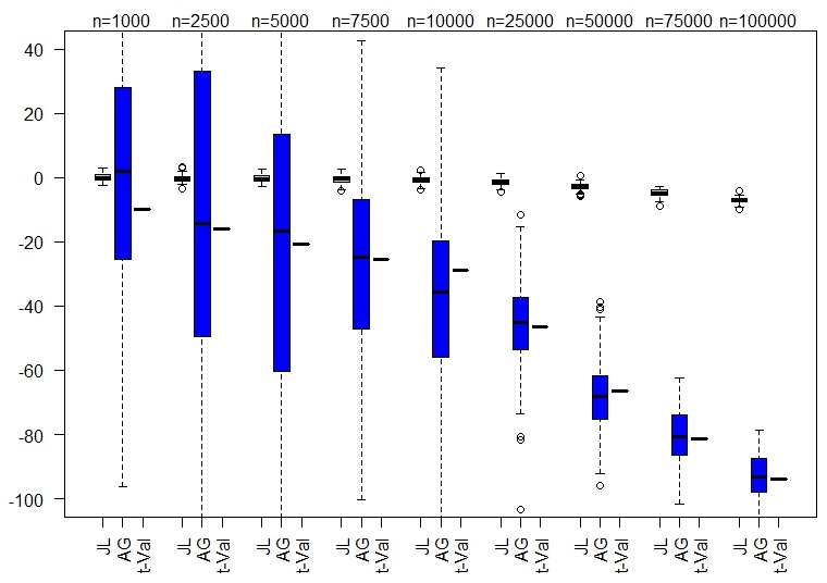
Results. We plot the tt-values we get from Algorithms 1 and 2 and decide to reject the null-hypothesis based on tt-value larger than 2.82.8 (which corresponds to a fairly conservative pp-value of 0.0050.005). Not surprisingly, as nn increases, the tt-values become closer to their expected value – the tt-value of Analyze Gauss is close to the non-private tt-value and the tt-value from Algorithm 1 is a factor of rn\sqrt{\tfrac{r}{n}} smaller as detailed above (see after Corollary 3.2). As a result, when the null-hypothesis is false, Analyze Gauss tends to produce larger tt-values (and thus reject the null-hypothesis) for values of nn under which Algorithm 1 still does not reject, as shown in Figure 1(a). This is exacerbated in real data setting, where its actual least singular value (≈500\approx 500) is fairly small in comparison to its size (N=91842N=91842).

However, what is fairly surprising is the case where the null-hypothesis should not be rejected — since βj=0\beta_{j}=0 (in the synthetic case) or its non-private tt-value is close to 00 (in the real-data case). Here, the Analyze Gauss’ tt-value approximation has fairly large variance, and we still get fairly high (in magnitude) tt-values. As the result, we falsely reject the null-hypothesis based on the tt-value of Analyze Gauss quite often, even for large values of nn. This is shown in Figure 1(b). Additional figures (including plotting the distribution of the tt-value approximations) appear in the supplementary material.

The results show that tt-value approximations that do not take into account the inherent randomness in the DP-algorithms lead to erroneous conclusions. One approach would be to follow the more conservative approach we advocate in this paper, where Algorithm 1 may allow you to get true approximation of the tt-values and otherwise reject the null-hypothesis only based on the confidence interval (of Algorithm 1 or 2) not intersecting the origin. Another approach, which we leave as future work, is to replace the TT-distribution with a new distribution, one that takes into account the randomness in the estimator as well. This, however, has been an open and long-standing challenge since the first works on DP and statistics (see (Vu & Slavkovic, 2009; Dwork & Lei, 2009)) and requires we move into non-asymptotic hypothesis testing.

Refer to caption
(a) Synthetic data, coordinate β1\beta_{1}
Refer to caption
(b) Synthetic data, coordinate β3\beta_{3}
Figure 1: Correctly and Wrongly Rejecting the Null-Hypothesis

Acknowledgements

The bulk of this work was done when the author was a postdoctoral fellow at Harvard University, supported by NSF grant CNS-123723; and also an unpaid collaborator on NSF grant 1565387. The author wishes to wholeheartedly thank Prof. Salil Vadhan, for his tremendous help in shaping this paper. The author would also like to thank Prof. Jelani Nelson and the members of the “Privacy Tools for Sharing Research Data” project at Harvard University (especially James Honaker, Vito D’Orazio, Vishesh Karwa, Prof. Kobbi Nissim and Prof. Gary King) for many helpful discussions and suggestions; as well as Abhradeep Thakurta for clarifying the similarity between our result. Lastly the author thanks the anonymous referees for many helpful suggestions in general and for a reference to (Ullman, 2015) in particular.

References

  • Agresti & Finlay (2009) Agresti, A. and Finlay, B. Statistical Methods for the Social Sciences. Pearson P. Hall, 2009.
  • Bassily et al. (2014) Bassily, R., Smith, A., and Thakurta, A. Private empirical risk minimization: Efficient algorithms and tight error bounds. In FOCS, 2014.
  • Blocki et al. (2012) Blocki, J., Blum, A., Datta, A., and Sheffet, O. The Johnson-Lindenstrauss transform itself preserves differential privacy. In FOCS, 2012.
  • Chaudhuri & Hsu (2012) Chaudhuri, Kamalika and Hsu, Daniel J. Convergence rates for differentially private statistical estimation. In ICML, 2012.
  • Chaudhuri et al. (2011) Chaudhuri, Kamalika, Monteleoni, Claire, and Sarwate, Anand D. Differentially private empirical risk minimization. Journal of Machine Learning Research, 12, 2011.
  • Duchi et al. (2013) Duchi, John C., Jordan, Michael I., and Wainwright, Martin J. Local privacy and statistical minimax rates. In FOCS, pp. 429–438, 2013.
  • Dwork & Lei (2009) Dwork, C. and Lei, J. Differential privacy and robust statistics. In STOC, 2009.
  • Dwork et al. (2006a) Dwork, Cynthia, Kenthapadi, Krishnaram, McSherry, Frank, Mironov, Ilya, and Naor, Moni. Our data, ourselves: Privacy via distributed noise generation. In EUROCRYPT, 2006a.
  • Dwork et al. (2006b) Dwork, Cynthia, Mcsherry, Frank, Nissim, Kobbi, and Smith, Adam. Calibrating noise to sensitivity in private data analysis. In TCC, 2006b.
  • Dwork et al. (2014) Dwork, Cynthia, Talwar, Kunal, Thakurta, Abhradeep, and Zhang, Li. Analyze gauss - optimal bounds for privacy preserving principal component analysis. In STOC, 2014.
  • Dwork et al. (2015) Dwork, Cynthia, Su, Weijie, and Zhang, Li. Private false discovery rate control. CoRR, abs/1511.03803, 2015.
  • Hoerl & Kennard (1970) Hoerl, A. E. and Kennard, R. W. Ridge regression: Biased estimation for nonorthogonal problems. Technometrics, 12:55–67, 1970.
  • Kasiviswanathan et al. (2008) Kasiviswanathan, S., Lee, H., Nissim, K., Raskhodnikova, S., and Smith, A. What can we learn privately? In FOCS, 2008.
  • Kifer et al. (2012) Kifer, Daniel, Smith, Adam D., and Thakurta, Abhradeep. Private convex optimization for empirical risk minimization with applications to high-dimensional regression. In COLT, 2012.
  • Laurent & Massart (2000) Laurent, B. and Massart, P. Adaptive estimation of a quadratic functional by model selection. The Annals of Statistics, 28(5), 10 2000.
  • Ma & Zarowski (1995) Ma, E. M. and Zarowski, Christopher J. On lower bounds for the smallest eigenvalue of a hermitian positive-definite matrix. IEEE Transactions on Information Theory, 41(2), 1995.
  • Muller & Stewart (2006) Muller, Keith E. and Stewart, Paul W. Linear Model Theory: Univariate, Multivariate, and Mixed Models. John Wiley & Sons, Inc., 2006.
  • Pilanci & Wainwright (2014a) Pilanci, M. and Wainwright, M. Randomized sketches of convex programs with sharp guarantees. In ISIT, 2014a.
  • Pilanci & Wainwright (2014b) Pilanci, Mert and Wainwright, Martin J. Iterative hessian sketch: Fast and accurate solution approximation for constrained least-squares. CoRR, abs/1411.0347, 2014b.
  • Rao (1973) Rao, C. Radhakrishna. Linear statistical inference and its applications. Wiley, 1973.
  • Rogers et al. (2016) Rogers, Ryan M., Vadhan, Salil P., Lim, Hyun-Woo, and Gaboardi, Marco. Differentially private chi-squared hypothesis testing: Goodness of fit and independence testing. In ICML, pp. 2111–2120, 2016.
  • Rudelson & Vershynin (2009) Rudelson, Mark and Vershynin, Roman. Smallest singular value of a random rectangular matrix. Comm. Pure Appl. Math, pp. 1707–1739, 2009.
  • Sarlós (2006) Sarlós, T. Improved approx. algs for large matrices via random projections. In FOCS, 2006.
  • Sheffet (2015) Sheffet, O. Private approximations of the 2nd-moment matrix using existing techniques in linear regression. CoRR, abs/1507.00056, 2015. URL http://arxiv.org/abs/1507.00056.
  • Smith (2011) Smith, Adam D. Privacy-preserving statistical estimation with optimal convergence rates. In STOC, pp. 813–822, 2011.
  • Strack et al. (2014) Strack, B., DeShazo, J., Gennings, C., Olmo, J., Ventura, S., Cios, K., and Clore, J. Impact of HbA1c measurement on hospital readmission rates: Analysis of 70,000 clinical database patient records. BioMed Research International, 2014:11 pages, 2014.
  • Tao (2012) Tao, T. Topics in Random Matrix Theory. American Mathematical Soc., 2012.
  • Thakurta & Smith (2013) Thakurta, Abhradeep and Smith, Adam. Differentially private feature selection via stability arguments, and the robustness of the lasso. In COLT, 2013.
  • Tikhonov (1963) Tikhonov, A. N. Solution of incorrectly formulated problems and the regularization method. Soviet Math. Dokl., 4, 1963.
  • Uhler et al. (2013) Uhler, Caroline, Slavkovic, Aleksandra B., and Fienberg, Stephen E. Privacy-preserving data sharing for genome-wide association studies. Journal of Privacy and Confidentiality, 2013. Available at: http://repository.cmu.edu/jpc/vol5/iss1/6.
  • Ullman (2015) Ullman, J. Private multiplicative weights beyond linear queries. In PODS, 2015.
  • Vu & Slavkovic (2009) Vu, D. and Slavkovic, A. Differential privacy for clinical trial data: Preliminary evaluations. In ICDM, 2009.
  • Wang et al. (2015) Wang, Yue, Lee, Jaewoo, and Kifer, Daniel. Differentially private hypothesis testing, revisited. CoRR, abs/1511.03376, 2015.
  • Xi et al. (2011) Xi, B., Kantarcioglu, M., and Inan, A. Mixture of gaussian models and bayes error under differential privacy. In CODASPY. ACM, 2011.
  • Zhou et al. (2007) Zhou, S., Lafferty, J., and Wasserman, L. Compressed regression. In NIPS, 2007.

Appendix A Extended Introductory Discussion

Due to space constraint, a few details from the introductory parts (Sections 1,2) were omitted. We bring them in this appendix. We especially recommend the uninformed reader to go over the extended OLS background we provide in Appendix A.3.

A.1 Proof Of Privacy of Algorithm 1

Theorem A.1.

Algorithm 1 is (ϵ,δ)(\epsilon,\delta)-differentially private.

Proof.

The proof of the theorem is based on the fact the Algorithm 1 is the result of composing the differentially private Propose-Test-Release algorithm of (Dwork & Lei, 2009) with the differentially private analysis of the Johnson-Lindenstrauss transform of (Sheffet, 2015).

More specifically, we use Theorem B.1 from (Sheffet, 2015) that states that given a matrix AA whose all of its singular values at greater than T⁡(ϵ,δ)T(\epsilon,\delta) where T​(ϵ,δ)2=2​B2ϵ​(2​r​ln⁡(4/δ)+2​ln⁡(4/δ))T(\epsilon,\delta)^{2}=\frac{2B^{2}}{\epsilon}\left(\sqrt{2r\ln(4/\delta)}+2\ln(4/\delta)\right), publishing R​ARA is (ϵ,δ)(\epsilon,\delta)-differentially private for a rr-row matrix RR whose entries sampled are i.i.d normal Gaussians. Since we have that all of the singular values of A′A^{\prime} are greater than ww (as specified in Algorithm 1), outputting R​A′RA^{\prime} is (ϵ/2,δ/2)(\epsilon/2,\delta/2)-differentially private. The rest of the proof boils down to showing that (i) the if-else-condition is (ϵ/2,0)(\epsilon/2,0)-differentially private and that (ii) w.p. ≤δ/2\leq\delta/2 any matrix AA whose smallest singular value is smaller than ww passes the if-condition (step 3). If both these facts hold, then knowing whether we pass the if-condition or not is (ϵ/2CLOSE(\epsilon/2)-differentially private and the output of the algorithm is (ϵ/2,δ)(\epsilon/2,\delta)-differentially private, hence basic composition gives the overall bound of (ϵ,δ)(\epsilon,\delta)-differential privacy.

To prove (i) we have that for any pair of neighboring matrices AA and BB that differ only on the ii-th row, denoted 𝒂i\boldsymbol{a}_{i} and 𝒃i\boldsymbol{b}_{i} resp., we have B𝖳​B−𝒃i​𝒃i𝖳=A𝖳​A−𝒂i​𝒂i𝖳B^{\mathsf{T}}B-\boldsymbol{b}_{i}\boldsymbol{b}_{i}^{\mathsf{T}}=A^{\mathsf{T}}A-\boldsymbol{a}_{i}\boldsymbol{a}_{i}^{\mathsf{T}}. Applying Weyl’s inequality we have

σmin​(B𝖳​B)\displaystyle\sigma_{\min}(B^{\mathsf{T}}B) ≤σmin​(B𝖳​B−𝒃i​𝒃i𝖳)+σmax​(𝒃i​𝒃i𝖳)\displaystyle\leq\sigma_{\min}(B^{\mathsf{T}}B-\boldsymbol{b}_{i}\boldsymbol{b}_{i}^{\mathsf{T}})+\sigma_{\max}(\boldsymbol{b}_{i}\boldsymbol{b}_{i}^{\mathsf{T}})
≤σmin​(A𝖳​A)+σmax​(𝒂i​𝒂i𝖳)+σmax​(𝒃i​𝒃i𝖳)\displaystyle\leq\sigma_{\min}(A^{\mathsf{T}}A)+\sigma_{\max}(\boldsymbol{a}_{i}\boldsymbol{a}_{i}^{\mathsf{T}})+\sigma_{\max}(\boldsymbol{b}_{i}\boldsymbol{b}_{i}^{\mathsf{T}})
≤σmin​(A𝖳​A)+2​B2\displaystyle\leq\sigma_{\min}(A^{\mathsf{T}}A)+2B^{2}

hence |σmin​(A)2−σmin​(B)2|≤2​B2|\sigma_{\min}(A)^{2}-\sigma_{\min}(B)^{2}|\leq 2B^{2}, so adding L​a​p​(4​B2ϵ)Lap(\frac{4B^{2}}{\epsilon}) is (ϵ/2)(\epsilon/2)-differentially private.

To prove (ii), note that by standard tail-bounds on the Laplace distribution we have that 𝐏𝐫[Z<−4​B2​ln⁡(1/δ)ϵ]≤δ2{\bf Pr}[Z~<~-\frac{4B^{2}\ln(1/\delta)}{\epsilon}]\leq\tfrac{\delta}{2}. Therefore, w.p. 1−δ/21-\delta/2 it holds that any matrix AA that passes the if-test of the algorithm must have σmin​(A)2>w2\sigma_{\min}(A)^{2}>w^{2}. Also note that a similar argument shows that for any 0<β<10<\beta<1, any matrix AA s.t. σmin​(A)2>w2+4​B2​ln⁡(1/β)ϵ\sigma_{\min}(A)^{2}>w^{2}+\frac{4B^{2}\ln(1/\beta)}{\epsilon} passes the if-condition of the algorithm w.p. 1−β1-\beta. ∎

A.2 Omitted Preliminary Details

Linear Algebra and Pseudo-Inverses. Given a matrix MM we denote its SVD as M=U​S​V𝖳M=USV^{\mathsf{T}} with UU and VV being orthonormal matrices and SS being a non-negative diagonal matrix whose entries are the singular values of MM. We use σmax​(M)\sigma_{\max}(M) and σmin​(M)\sigma_{\min}(M) to denote the largest and smallest singular value resp. Despite the risk of confusion, we stick to the standard notation of using σ2\sigma^{2} to denote the variance of a Gaussian, and use σj​(M)\sigma_{j}(M) to denote the jj-th singular value of MM. We use M+M^{+} to denote the Moore-Penrose inverse of MM, defined as M+=V​S−1​UTM^{+}=VS^{-1}U^{T} where S−1S^{-1} is a matrix with Sj,j−1=1/Sj,jS^{-1}_{j,j}=1/S_{j,j} for any jj s.t. Sj,j>0S_{j,j}>0.

The Gaussian Distribution. A univariate Gaussian 𝒩⁡(μ,σ2){\mathcal{N}}(\mu,\sigma^{2}) denotes the Gaussian distribution whose mean is μ\mu and variance σ2\sigma^{2}, with 𝖯𝖣𝖥⁡(x)=(2​π​σ2)−1​exp⁡(−x−μ2​σ2)\mathsf{PDF}(x)=(\sqrt{2\pi\sigma^{2}})^{-1}\exp(-\tfrac{x-\mu}{2\sigma^{2}}). Standard concentration bounds on Gaussians give that 𝐏𝐫[x>μ+2σln⁡(1/ν)]<ν{\bf Pr}[x>\mu+2\sigma\sqrt{\ln(1/\nu)}]<\nu for any ν∈(0,1e)\nu\in(0,\tfrac{1}{e}). A multivariate Gaussian 𝒩⁡(𝝁,Σ){\mathcal{N}}(\boldsymbol{\mu},\Sigma) for some positive semi-definite Σ\Sigma denotes the multivariate Gaussian distribution where the mean of the jj-th coordinate is the μj\mu_{j} and the co-variance between coordinates jj and kk is Σj,k\Sigma_{j,k}. The 𝖯𝖣𝖥\mathsf{PDF} of such Gaussian is defined only on the subspace c​o​l​s​p​a​n​(Σ)colspan(\Sigma), where for every x∈c​o​l​s​p​a​n​(Σ)x\in colspan(\Sigma) we have 𝖯𝖣𝖥(𝒙)=((2π)r​a​n​k​(Σ)⋅det~(Σ))−1/2exp(−12(𝒙−𝝁)𝖳Σ+(𝒙−𝝁))\mathsf{PDF}(\boldsymbol{x})=\left((2\pi)^{rank(\Sigma)}\cdot\tilde{\det}(\Sigma)\right)^{-1/2}\exp\left(-\tfrac{1}{2}(\boldsymbol{x}-\boldsymbol{\mu})^{\mathsf{T}}\Sigma^{+}(\boldsymbol{x}-\boldsymbol{\mu})\right) and det~​(Σ)\tilde{\det}(\Sigma) is the multiplication of all non-zero singular values of Σ\Sigma. A matrix Gaussian distribution denoted 𝒩⁡(Ma×b,U,V){\mathcal{N}}(M_{a\times b},U,V) has mean MM, variance UU on its rows and variance VV on its columns. For full rank UU and VV it holds that 𝖯𝖣𝖥𝒩⁡(M,U,V)(X)=(2π)−ab/2(det(U))−b/2(det(V))−a/2⋅exp(−12trace(V−1(X−M)𝖳U−1(X−M)))\mathsf{PDF}_{{\mathcal{N}}(M,U,V)}(X)=(2\pi)^{-ab/2}(\det(U))^{-b/2}(\det(V))^{-a/2}\cdot\exp(-\tfrac{1}{2}\mathrm{trace}\left(V^{-1}(X-M)^{\mathsf{T}}U^{-1}(X-M)\right)). In our case, we will only use matrix Gaussian distributions with 𝒩⁡(Ma×b,Ia×a,V){\mathcal{N}}(M_{a\times b},I_{a\times a},V) and so each row in this matrix is an i.i.d sample from a bb-dimensional multivariate Gaussian 𝒩⁡((M)j→,V){\mathcal{N}}((M)_{j\to},V).

We will repeatedly use the rules regarding linear operations on Gaussians. That in, for any cc, it holds that c​𝒩​(μ,σ2)=𝒩⁡(c⋅μ,c2​σ2)c{\mathcal{N}}(\mu,\sigma^{2})={\mathcal{N}}(c\cdot\mu,c^{2}\sigma^{2}). For any CC it holds that C⋅𝒩⁡(𝝁,Σ)=𝒩⁡(C​𝝁,C​Σ​C𝖳)C\cdot{\mathcal{N}}(\boldsymbol{\mu},\Sigma)={\mathcal{N}}(C\boldsymbol{\mu},C\Sigma C^{\mathsf{T}}). And for any CC is holds that 𝒩⁡(M,U,V)⋅C=𝒩⁡(M​C,U,C𝖳​V​C){\mathcal{N}}(M,U,V)\cdot C={\mathcal{N}}(MC,U,C^{\mathsf{T}}VC). In particular, for any 𝒄\boldsymbol{c} (which can be viewed as a b×1b\times 1-matrix) it holds that 𝒩⁡(M,U,V)⋅𝒄=𝒩⁡(M​𝒄,U,𝒄T​V​𝒄)=𝒩⁡(M​𝒄,𝒄T​V​𝒄⋅U){\mathcal{N}}(M,U,V)\cdot\boldsymbol{c}={\mathcal{N}}(M\boldsymbol{c},U,\boldsymbol{c}^{T}V\boldsymbol{c})={\mathcal{N}}(M\boldsymbol{c},\boldsymbol{c}^{T}V\boldsymbol{c}\cdot U).

We will also require the following proposition.

Proposition A.2.

Given σ2,λ2\sigma^{2},\lambda^{2} s.t. 1≤σ2λ2≤c21\leq\frac{\sigma^{2}}{\lambda^{2}}\leq c^{2} for some constant cc, let XX and YY be two random Gaussians s.t. X∼𝒩⁡(0,σ2)X\sim{\mathcal{N}}(0,\sigma^{2}) and Y∼𝒩⁡(0,λ2)Y\sim{\mathcal{N}}(0,\lambda^{2}). It follows that 1c​𝖯𝖣𝖥Y​(x)≤𝖯𝖣𝖥X​(x)≤c​𝖯𝖣𝖥c​Y​(x)\tfrac{1}{c}\mathsf{PDF}_{Y}(x)\leq\mathsf{PDF}_{X}(x)\leq c\mathsf{PDF}_{cY}(x) for any xx.

Corollary A.3.

Under the same notation as in Proposition A.2, for any set S⊂ℝS\subset\mathbb{R} it holds that 1c𝐏𝐫x←Y[x∈S]≤𝐏𝐫x←X[x∈S]≤c𝐏𝐫x←c​Y[x∈S]=c𝐏𝐫x←Y[x∈S/c]\tfrac{1}{c}{\bf Pr}_{x\leftarrow Y}[x\in S]\leq{\bf Pr}_{x\leftarrow X}[x\in S]\leq c{\bf Pr}_{x\leftarrow cY}[x\in S]=c{\bf Pr}_{x\leftarrow Y}[x\in S/c]

Proof.

The proof is mere calculation.

𝖯𝖣𝖥X​(x)𝖯𝖣𝖥c​Y​(x)\displaystyle\frac{\mathsf{PDF}_{X}(x)}{\mathsf{PDF}_{cY}(x)} =c2​λ2σ2⋅exp⁡(−x22​σ2)exp⁡(−x22​c2​λ2)\displaystyle=\sqrt{\frac{c^{2}\lambda^{2}}{\sigma^{2}}}\cdot\frac{\exp(-\tfrac{x^{2}}{2\sigma^{2}})}{\exp(-\tfrac{x^{2}}{2c^{2}\lambda^{2}})}
≤c⋅exp⁡(x22​(1c2​λ2−1σ2))≤c⋅exp⁡(0)=c\displaystyle\leq c\cdot\exp(\frac{x^{2}}{2}(\frac{1}{c^{2}\lambda^{2}}-\frac{1}{\sigma^{2}}))\leq c\cdot\exp(0)=c
𝖯𝖣𝖥X​(x)𝖯𝖣𝖥Y​(x)\displaystyle\frac{\mathsf{PDF}_{X}(x)}{\mathsf{PDF}_{Y}(x)} =λ2σ2⋅exp⁡(−x22​σ2)exp⁡(−x22​λ2)\displaystyle=\sqrt{\frac{\lambda^{2}}{\sigma^{2}}}\cdot\frac{\exp(-\tfrac{x^{2}}{2\sigma^{2}})}{\exp(-\tfrac{x^{2}}{2\lambda^{2}})}
≥c−1​exp⁡(x22​(1λ2−1σ2))≥exp⁡(0)c=c−1\displaystyle\geq c^{-1}\exp(\tfrac{x^{2}}{2}(\tfrac{1}{\lambda^{2}}-\tfrac{1}{\sigma^{2}}))\geq\tfrac{\exp(0)}{c}=c^{-1}

∎

The TkT_{k}-Distribution. The TkT_{k}-distribution, where kk is referred to as the degrees of freedom of the distribution, denotes the distribution over the reals created by independently sampling Z∼𝒩⁡(0,1)Z\sim{\mathcal{N}}(0,1) and ‖ζ‖2∼χk2\|\zeta\|^{2}\sim\chi^{2}_{k}, and taking the quantity Z‖ζ‖2/k\frac{Z}{\sqrt{\|\zeta\|^{2}/k}}. Its 𝖯𝖣𝖥\mathsf{PDF} is given by 𝖯𝖣𝖥Tk​(x)∝(1+x2k)−k+12\mathsf{PDF}_{T_{k}}(x)\propto\left(1+\tfrac{x^{2}}{k}\right)^{-\tfrac{k+1}{2}}. It is a known fact that as kk increases, TkT_{k} becomes closer and closer to a normal Gaussian. The TT-distribution is often used to determine suitable bounds on the rate of converges, as we illustrate in Section A.3. As the TT-distribution is heavy-tailed, existing tail bounds on the TT-distribution (which are of the form: if τν=C​k⁡((1/ν)2/k−1)\tau_{\nu}=C\sqrt{k((1/\nu)^{2/k}-1)} for some constant CC then ∫τν∞𝖯𝖣𝖥Tk​(x)​𝑑x<ν\int_{\tau_{\nu}}^{\infty}\mathsf{PDF}_{T_{k}}(x)dx<\nu) are often cumbersome to work with. Therefore, in many cases in practice, it common to assume ν=Θ⁡(1)\nu=\Theta(1) (most commonly, ν=0.05\nu=0.05) and use existing tail-bounds on normal Gaussians.

Differential Privacy facts. It is known (Dwork et al., 2006b) that if 𝖠𝖫𝖦\mathsf{ALG} outputs a vector in ℝd\mathbb{R}^{d} such that for any AA and A′A^{\prime} it holds that ‖𝖠𝖫𝖦⁡(A)−𝖠𝖫𝖦⁡(A′)‖1≤B\|\mathsf{ALG}(A)-\mathsf{ALG}(A^{\prime})\|_{1}\leq B, then adding Laplace noise L​a​p​(1/ϵ)Lap(1/\epsilon) to each coordinate of the output of 𝖠𝖫𝖦⁡(A)\mathsf{ALG}(A) satisfies ϵ\epsilon-differential privacy. Similarly, (2006b) showed that if for any neighboring AA and A′A^{\prime} it holds that ‖𝖠𝖫𝖦⁡(A)−𝖠𝖫𝖦⁡(A′)‖22≤Δ2\|\mathsf{ALG}(A)-\mathsf{ALG}(A^{\prime})\|_{2}^{2}\leq\Delta^{2} then adding Gaussian noise 𝒩⁡(0,Δ2⋅2​ln⁡(2/δ)ϵ2){\mathcal{N}}(0,\Delta^{2}\cdot\tfrac{2\ln(2/\delta)}{\epsilon^{2}}) to each coordinate of the output of 𝖠𝖫𝖦⁡(A)\mathsf{ALG}(A) satisfies (ϵ,δ)(\epsilon,\delta)-differential privacy.

Another standard result (Dwork et al., 2006a) gives that the composition of the output of a (ϵ1,δ1)(\epsilon_{1},\delta_{1})-differentially private algorithm with the output of a (ϵ2,δ2)(\epsilon_{2},\delta_{2})-differentially private algorithm results in a (ϵ1+ϵ2,δ1+δ2)(\epsilon_{1}+\epsilon_{2},\delta_{1}+\delta_{2})-differentially private algorithm.

A.3 Detailed Background on Ordinary Least Squares

For the unfamiliar reader, we give a short description of the model under which OLS operates as well as the confidence bounds one derives using OLS. This is by no means an exhaustive account of OLS and we refer the interested reader to (Rao, 1973; Muller & Stewart, 2006).

Given nn observations {(𝒙i,yi)}i=1n\{(\boldsymbol{x}_{i},y_{i})\}_{i=1}^{n} where for all ii we have 𝒙i∈ℝp\boldsymbol{x}_{i}\in\mathbb{R}^{p} and yi∈ℝy_{i}\in\mathbb{R}, we assume the existence of a pp-dimensional vector 𝜷∈ℝp\boldsymbol{\beta}\in\mathbb{R}^{p} s.t. the label yiy_{i} was derived by yi=𝜷𝖳​𝒙i+eiy_{i}=\boldsymbol{\beta}^{\mathsf{T}}\boldsymbol{x}_{i}+e_{i} where ei∼𝒩⁡(0,σ2)e_{i}\sim{\mathcal{N}}(0,\sigma^{2}) independently (also known as the homoscedastic Gaussian model). We use the matrix notation where XX denotes the (n×p)(n\times p)-matrix whose rows are 𝒙i\boldsymbol{x}_{i}, and use 𝒚,𝒆∈ℝn\boldsymbol{y},\boldsymbol{e}\in\mathbb{R}^{n} to denote the vectors whose ii-th entry is yiy_{i} and eie_{i} resp. To simplify the discussion, we assume XX has full rank.

The parameters of the model are therefore 𝜷\boldsymbol{\beta} and σ2\sigma^{2}, which we set to discover. To that end, we minimize min𝒛⁡‖𝒚−X​𝒛‖2\min_{\boldsymbol{z}}\|\boldsymbol{y}-X\boldsymbol{z}\|^{2} and solve

𝜷^=(X𝖳​X)−1​X𝖳​𝒚=(X𝖳​X)−1​X𝖳​(X​𝜷+𝒆)=𝜷+X+​𝒆\hat{\boldsymbol{\beta}}=(X^{\mathsf{T}}X)^{-1}X^{\mathsf{T}}\boldsymbol{y}=(X^{\mathsf{T}}X)^{-1}X^{\mathsf{T}}(X\boldsymbol{\beta}+\boldsymbol{e})=\boldsymbol{\beta}+X^{+}\boldsymbol{e}

As 𝒆∼𝒩⁡(𝟎n,σ2​In×n)\boldsymbol{e}\sim{\mathcal{N}}(\boldsymbol{0}_{n},\sigma^{2}I_{n\times n}), it holds that 𝜷^∼𝒩⁡(𝜷,σ2​(X𝖳​X)−1)\hat{\boldsymbol{\beta}}\sim{\mathcal{N}}(\boldsymbol{\beta},\sigma^{2}(X^{\mathsf{T}}X)^{-1}), or alternatively, that for every coordinate jj it holds that β^j=𝒆j𝖳​𝜷^∼𝒩⁡(βj,σ2​(X𝖳​X)j,j−1)\hat{\beta}_{j}=\boldsymbol{e}_{j}^{\mathsf{T}}\hat{\boldsymbol{\beta}}\sim{\mathcal{N}}(\beta_{j},\sigma^{2}(X^{\mathsf{T}}X)^{-1}_{j,j}). Hence we get β^j−βjσ​(X𝖳​X)j,j−1∼𝒩⁡(0,1)\frac{\hat{\beta}_{j}-\beta_{j}}{\sigma\sqrt{(X^{\mathsf{T}}X)^{-1}_{j,j}}}\sim{\mathcal{N}}(0,1). In addition, we denote the vector

𝜻=y−X​𝜷^=(X​𝜷+𝒆)−X⁡(𝜷+X+​𝒆)=(I−X​X+)​𝒆\boldsymbol{\zeta}=y-X\hat{\boldsymbol{\beta}}=(X\boldsymbol{\beta}+\boldsymbol{e})-X(\boldsymbol{\beta}+X^{+}\boldsymbol{e})=(I-XX^{+})\boldsymbol{e}

and since X​X+XX^{+} is a rank-pp (symmetric) projection matrix, we have 𝜻∼𝒩⁡(0,σ2​(I−X​X+))\boldsymbol{\zeta}\sim{\mathcal{N}}(0,\sigma^{2}(I-XX^{+})). Therefore, ‖𝜻‖2\|\boldsymbol{\zeta}\|^{2} is equivalent to summing the squares of (n−p)(n-p) i.i.d samples from 𝒩⁡(0,σ2){\mathcal{N}}(0,\sigma^{2}). In other words, the quantity ‖𝜻‖2/σ2\|\boldsymbol{\zeta}\|^{2}/\sigma^{2} is sampled from a χ2\chi^{2}-distribution with (n−p)(n-p) degrees of freedom.

We sidetrack from the OLS discussion to give the following bounds on the l2l_{2}-distance between 𝜷\boldsymbol{\beta} and 𝜷^\hat{\boldsymbol{\beta}}, as the next claim shows.

Claim A.4.

For any 0<ν<1/20<\nu<1/2, the following holds w.p. ≥1−ν\geq 1-\nu over the randomness of the model (the randomness over 𝐞\boldsymbol{e})

‖𝜷−𝜷^‖2\displaystyle{\|\boldsymbol{\beta}-\hat{\boldsymbol{\beta}}\|^{2}} =‖X+​𝒆‖2\displaystyle=\|X^{+}\boldsymbol{e}\|^{2} (7)
=O⁡(σ2​log⁡(p/ν)⋅‖X+‖F2)\displaystyle=O\left(\sigma^{2}\log(p/\nu)\cdot\|X^{+}\|_{F}^{2}\right) (8)
‖𝜷^‖2\displaystyle\|\hat{\boldsymbol{\beta}}\|^{2} =‖𝜷+X+​𝒆‖2\displaystyle=\|\boldsymbol{\beta}+X^{+}\boldsymbol{e}\|^{2} (9)
=O⁡((‖𝜷‖+σ⋅‖X+‖F⋅log⁡(p/ν))2)\displaystyle=O(\left(\|\boldsymbol{\beta}\|+\sigma\cdot\|X^{+}\|_{F}\cdot\sqrt{\log(p/\nu)}\right)^{2}) (10)
|1n−p​‖𝜻‖2−σ2|\displaystyle\left|\tfrac{1}{n-p}\|\boldsymbol{\zeta}\|^{2}-\sigma^{2}\right| =O⁡(ln⁡(1/ν)n−p)\displaystyle=O(\sqrt{\tfrac{\ln(1/\nu)}{n-p}})
Proof.

Since 𝒆∼𝒩⁡(𝟎n,σ2​In×n)\boldsymbol{e}\sim{\mathcal{N}}(\boldsymbol{0}_{n},\sigma^{2}I_{n\times n}) then X+​𝒆∼𝒩⁡(𝟎n,σ2​(X𝖳​X)−1)X^{+}\boldsymbol{e}\sim{\mathcal{N}}(\boldsymbol{0}_{n},\sigma^{2}(X^{\mathsf{T}}X)^{-1}). Denoting the SVD decomposition (X𝖳​X)−1=V​S​V𝖳(X^{\mathsf{T}}X)^{-1}=VSV^{\mathsf{T}} with SS denoting the diagonal matrix whose entries are σmax−2​(X),…,σmin−2​(X)\sigma_{\max}^{-2}(X),\ldots,\sigma_{\min}^{-2}(X), we have that V𝖳​X+​𝒆∼𝒩⁡(𝟎n,σ2​S)V^{\mathsf{T}}X^{+}\boldsymbol{e}\sim{\mathcal{N}}(\boldsymbol{0}_{n},\sigma^{2}S). And so, each coordinate of V𝖳​X+​𝒆V^{\mathsf{T}}X^{+}\boldsymbol{e} is distributed like an i.i.d Gaussian. So w.p. ≥1−ν/2\geq 1-\nu/2 non of these Gaussians is a factor of O⁡(σ​ln⁡(p/ν))O(\sigma\sqrt{\ln(p/\nu)}) greater than its standard deviation. And so w.p. ≥1−ν/2\geq 1-\nu/2 it holds that ‖X+​𝒆‖2=‖V𝖳​X+​𝒆‖2≤O⁡(σ2​log⁡(p/ν)​(∑iσi−2​(X)))\|X^{+}\boldsymbol{e}\|^{2}=\|V^{\mathsf{T}}X^{+}\boldsymbol{e}\|^{2}\leq O(\sigma^{2}\log(p/\nu)\left(\sum_{i}\sigma_{i}^{-2}(X)\right)). Since ∑iσi−2​(X)=trace⁡((X𝖳​X)−1)=trace⁡(X+​(X+)𝖳)=‖X+‖F2\sum_{i}\sigma_{i}^{-2}(X)=\mathrm{trace}((X^{\mathsf{T}}X)^{-1})=\mathrm{trace}(X^{+}(X^{+})^{\mathsf{T}})=\|X^{+}\|_{F}^{2}, the bound of (8) is proven.

The bound on ‖𝜷^‖2\|\hat{\boldsymbol{\beta}}\|^{2} is an immediate corollary of (8) using the triangle inequality.88 8 Observe, though 𝒆\boldsymbol{e} is spherically symmetric, and is likely to be approximately-orthogonal to 𝜷\boldsymbol{\beta}, this does not necessarily hold for X+​𝒆X^{+}\boldsymbol{e} which isn’t spherically symmetric. Therefore, we result to bounding the l2l_{2}-norm of 𝜷^\hat{\boldsymbol{\beta}} using the triangle bound. The bound on ‖𝜻‖2\|\boldsymbol{\zeta}\|^{2} follows from tail bounds on the χn−p2\chi^{2}_{n-p} distribution, as detailed in Section 2. ∎

Returning to OLS, it is important to note that 𝜷^\hat{\boldsymbol{\beta}} and 𝜻\boldsymbol{\zeta} are independent of one another. (Note, 𝜷^\hat{\boldsymbol{\beta}} depends solely on X+​𝒆=(X+​X)​X+​𝒆=X+​PU​𝒆X^{+}\boldsymbol{e}=(X^{+}X)X^{+}\boldsymbol{e}=X^{+}P_{U}\boldsymbol{e}, whereas 𝜻\boldsymbol{\zeta} depends on (I−X​X+)​𝒆=PU⟂​𝒆(I-XX^{+})\boldsymbol{e}=P_{U^{\perp}}\boldsymbol{e}. As 𝒆\boldsymbol{e} is spherically symmetric, the two projections are independent of one another and so 𝜷^\hat{\boldsymbol{\beta}} is independent of 𝜻\boldsymbol{\zeta}.) As a result of the above two calculations, we have that the quantity

tβ^j​(βj)=defβ^j−βj(X𝖳​X)j,j−1⋅‖𝜻‖n−p=β^j−βjσ​(X𝖳​X)j,j−1/‖𝜻‖σ​n−pt_{\hat{\beta}_{j}}(\beta_{j})\stackrel{{\scriptstyle\rm def}}{{=}}\frac{\hat{\beta}_{j}-\beta_{j}}{\sqrt{(X^{\mathsf{T}}X)^{-1}_{j,j}}\cdot\frac{\|\boldsymbol{\zeta}\|}{\sqrt{n-p}}}=\frac{\hat{\beta}_{j}-\beta_{j}}{\sigma\sqrt{(X^{\mathsf{T}}X)^{-1}_{j,j}}}\Big/\frac{\|\boldsymbol{\zeta}\|}{\sigma\sqrt{n-p}}

is distributed like a TT-distribution with (n−p)(n-p) degrees of freedom. Therefore, we can compute an exact probability estimation for this quantity. That is, for any measurable S⊂ℝS\subset\mathbb{R} we have

𝐏𝐫[𝜷^ and 𝜻 satisfying tβ^j(βj)∈S]=∫S𝖯𝖣𝖥Tn−p(x)dx{\bf Pr}\left[\hat{\boldsymbol{\beta}}\textrm{ and }\boldsymbol{\zeta}\textrm{ satisfying }t_{\hat{\beta}_{j}}(\beta_{j})\in S\right]=\int_{S}\mathsf{PDF}_{T_{n-p}}(x)dx

The importance of the tt-value t⁡(βj)t(\beta_{j}) lies in the fact that it can be fully estimated from the observed data XX and yy (for any value of βj\beta_{j}), which makes it a pivotal quantity. Therefore, given XX and 𝒚\boldsymbol{y}, we can use t⁡(βj)t(\beta_{j}) to describe the likelihood of any βj\beta_{j} — for any z∈ℝz\in\mathbb{R} we can now give an estimation of how likely it is to have βj=z\beta_{j}=z (which is 𝖯𝖣𝖥Tn−p​(t​(z))\mathsf{PDF}_{T_{n-p}}(t(z))). The tt-values enable us to perform multitude of statistical inferences. For example, we can say which of two hypotheses is more likely and by how much (e.g., we are 55-times more likely that the hypothesis βj=3\beta_{j}=3 is true than the hypothesis βj=14\beta_{j}=14 is true); we can compare between two coordinates jj and j′j^{\prime} and report we are more confident that βj>0\beta_{j}>0 than βj′>0\beta_{j^{\prime}}>0; or even compare among the tt-values we get across multiple datasets (such as the datasets we get from subsampling rows from a single dataset).

In particular, we can use t⁡(βj)t(\beta_{j}) to α\alpha-reject unlikely values of βj\beta_{j}. Given 0<α<10<\alpha<1, we denote cαc_{\alpha} as the number for which the interval (−cα,cα)(-c_{\alpha},c_{\alpha}) contains a probability mass of 1−α1-\alpha from the Tn−pT_{n-p}-distribution. And so we derive a corresponding confidence interval IαI_{\alpha} centered at β^j\hat{\beta}_{j} where βj∈Iα\beta_{j}\in I_{\alpha} with confidence of level of 1−α1-\alpha.

We comment as to the actual meaning of this confidence interval. Our analysis thus far applied w.h.p to a vector 𝒚\boldsymbol{y} derived according to this model. Such XX and 𝒚\boldsymbol{y} will result in the quantity tβ^j​(βj)t_{\hat{\beta}_{j}}(\beta_{j}) being distributed like a Tn−pT_{n-p}-distribution — where βj\beta_{j} is given as the model parameters and β^j\hat{\beta}_{j} is the random variable. We therefore have that guarantee that for XX and 𝒚\boldsymbol{y} derived according to this model, the event Eα=defβ^j∈(βj±cα⋅(X𝖳​X)j,j−1⋅‖𝜻‖2n−p)E_{\alpha}\stackrel{{\scriptstyle\rm def}}{{=}}\hat{\beta}_{j}\in\left(\beta_{j}\pm c_{\alpha}\cdot\sqrt{(X^{\mathsf{T}}X)^{-1}_{j,j}\cdot\tfrac{\|\boldsymbol{\zeta}\|^{2}}{n-p}}\right) happens w.p. 1−α1-\alpha. However, the analysis done over a given dataset XX and 𝒚\boldsymbol{y} (once 𝒚\boldsymbol{y} has been drawn) views the quantity tβ^j​(βj)t_{\hat{\beta}_{j}}(\beta_{j}) with β^j\hat{\beta}_{j} given and βj\beta_{j} unknown. Therefore the event EαE_{\alpha} either holds or does not hold. That is why the alternative terms of likelihood or confidence are used, instead of probability. We have a confidence level of 1−α1-\alpha that indeed βj∈βj^±cα⋅(X𝖳​X)j,j−1⋅‖𝜻‖2n−p\beta_{j}\in\hat{\beta_{j}}\pm c_{\alpha}\cdot\sqrt{(X^{\mathsf{T}}X)^{-1}_{j,j}\cdot\tfrac{\|\boldsymbol{\zeta}\|^{2}}{n-p}}, because this event does happen in 1−α1-\alpha fraction of all datasets generated according to our model.

Rejecting the Null Hypothesis. One important implication of the quantity t⁡(βj)t(\beta_{j}) is that we can refer specifically to the hypothesis that βj=0\beta_{j}=0, called the null hypothesis. This quantity, t0=deftβ^j​(0)=β^j​n−p‖𝜻‖​(X𝖳​X)j,j−1t_{0}\stackrel{{\scriptstyle\rm def}}{{=}}t_{\hat{\beta}_{j}}(0)=\frac{\hat{\beta}_{j}\sqrt{n-p}}{\|\boldsymbol{\zeta}\|\sqrt{(X^{\mathsf{T}}X)^{-1}_{j,j}}}, represents how large is β^j\hat{\beta}_{j} relatively to the empirical estimation of standard deviation σ\sigma. Since it is known that as the number of degrees of freedom of a TT-distribution tends to infinity then the TT-distribution becomes a normal Gaussian, it is common to think of t0t_{0} as a sample from a normal Gaussian 𝒩⁡(0,1){\mathcal{N}}(0,1). This allows us to associate t0t_{0} with a pp-value, estimating the event “βj\beta_{j} and β^j\hat{\beta}_{j} have different signs.” Formally, we define p0=∫|t0|∞12​πe−x2/2dxp_{0}=\int_{|t_{0}|}^{\infty}\frac{1}{\sqrt{2\pi}}e^{-x^{2}/2}dx. It is common to reject the null hypothesis when p0p_{0} is sufficiently small (typically, below 0.050.05).99 9 Indeed, it is more accurate to associate with t0t_{0} the value ∫|t0|∞𝖯𝖣𝖥Tn−p​(x)​𝑑x\int_{|t_{0}|}^{\infty}\mathsf{PDF}_{T_{n-p}}(x)dx and check that this value is <α<\alpha. However, as most uses take α\alpha to be a constant (often α=0.05\alpha=0.05), asymptotically the threshold we get for rejecting the null hypothesis are the same.

Specifically, given α∈(0,1/2)\alpha\in(0,1/2), we say we α\alpha-reject the null hypothesis if p0<αp_{0}<\alpha. Let τα\tau_{\alpha} be the number s.t. Φ(τα)=∫τα∞12​πe−x2/2dx=α\Phi(\tau_{\alpha})=\int_{\tau_{\alpha}}^{\infty}\tfrac{1}{\sqrt{2\pi}}e^{-x^{2}/2}dx=\alpha. (Standard bounds give that τα<2​ln⁡(1/α)\tau_{\alpha}<2\sqrt{\ln(1/\alpha)}.) This means we α\alpha-reject the null hypothesis if t0>ταt_{0}>\tau_{\alpha} or t0<−ταt_{0}<-\tau_{\alpha}, meaning if |β^j|>τα​(X𝖳​X)j,j−1​‖𝜻‖n−p|\hat{\beta}_{j}|>\tau_{\alpha}\sqrt{(X^{\mathsf{T}}X)^{-1}_{j,j}}\tfrac{\|\boldsymbol{\zeta}\|}{\sqrt{n-p}}.

We can now lower bound the number of i.i.d sample points needed in order to α\alpha-reject the null hypothesis. This bound will be our basis for comparison --- between standard OLS and the differentially private version.1010 10 This theorem is far from being new (except for maybe focusing on the setting where every row in XX is sampled from an i.i.d multivariate Gaussians), it is just stated in a non-standard way, discussing solely the power of the tt-test in OLS. For further discussions on sample size calculations see (Muller & Stewart, 2006).

Theorem A.5 (Theorem 2.2 restated.).

Fix any positive definite matrix Σ∈ℝp×p\Sigma\in\mathbb{R}^{p\times p} and any ν∈(0,12)\nu\in(0,\tfrac{1}{2}). Fix parameters 𝛃∈ℝp\boldsymbol{\beta}\in\mathbb{R}^{p} and σ2\sigma^{2} and a coordinate jj s.t. βj≠0\beta_{j}\neq 0. Let XX be a matrix whose nn rows are i.i.d samples from 𝒩⁡(𝟎,Σ){\mathcal{N}}(\boldsymbol{0},\Sigma), and 𝐲\boldsymbol{y} be a vector where yi−(X​𝛃)iy_{i}-(X\boldsymbol{\beta})_{i} is sampled i.i.d from 𝒩⁡(0,σ2){\mathcal{N}}(0,\sigma^{2}). Fix α∈(0,1)\alpha\in(0,1). Then w.p. ≥1−ν\geq 1-\nu we have that the (1−α)(1-\alpha)-confidence interval is of length 𝑂𝑃𝐸𝑁O⁡(cα​σ2/(n​σmin​(Σ)𝐶𝐿𝑂𝑆𝐸))O(c_{\alpha}\sqrt{\sigma^{2}/(n\sigma_{\min}(\Sigma)})) provided n≥C1​(p+ln⁡(1/ν))n\geq C_{1}(p+\ln(1/\nu)) for some sufficiently large constant C1C_{1}. Furthermore, there exists a constant C2C_{2} such that w.p. ≥1−α−ν\geq 1-\alpha-\nu we (correctly) reject the null hypothesis provided

n≥max⁡{C1​(p+ln⁡(1/ν)),C2​σ2βj2⋅cα2+τα2σmin​(Σ)}n\geq\max\left\{C_{1}(p+\ln(1/\nu)),~~C_{2}\frac{\sigma^{2}}{\beta_{j}^{2}}\cdot\frac{c_{\alpha}^{2}+\tau_{\alpha}^{2}}{\sigma_{\min}(\Sigma)}\right\}

Here cαc_{\alpha} denotes the number for which ∫−cαcα𝖯𝖣𝖥Tn−p​(x)​𝑑x=1−α\int_{-c_{\alpha}}^{c_{\alpha}}\mathsf{PDF}_{T_{n-p}}(x)dx=1-\alpha. (If we are content with approximating Tn−pT_{n-p} with a normal Gaussian than one can set cα≈τα<2​ln⁡(1/α)c_{\alpha}\approx\tau_{\alpha}<2\sqrt{\ln(1/\alpha)}.)

Proof.

The discussion above shows that w.p. ≥1−α\geq 1-\alpha we have |βj−β^j|≤cα​(X𝖳​X)j,j−1​‖𝜻‖2n−p|\beta_{j}-\hat{\beta}_{j}|\leq c_{\alpha}\sqrt{(X^{\mathsf{T}}X)^{-1}_{j,j}\tfrac{\|\boldsymbol{\zeta}\|^{2}}{n-p}}; and in order to α\alpha-reject the null hypothesis we must have |β^j|>τα​(X𝖳​X)j,j−1​‖𝜻‖2n−p|\hat{\beta}_{j}|>\tau_{\alpha}\sqrt{(X^{\mathsf{T}}X)^{-1}_{j,j}\tfrac{\|\boldsymbol{\zeta}\|^{2}}{n-p}}. Therefore, a sufficient condition for OLS to α\alpha-reject the null-hypothesis is to have nn large enough s.t. |βj|>(cα+τα)​(X𝖳​X)j,j−1​‖𝜻‖2n−p|\beta_{j}|>(c_{\alpha}+\tau_{\alpha})\sqrt{(X^{\mathsf{T}}X)^{-1}_{j,j}\tfrac{\|\boldsymbol{\zeta}\|^{2}}{n-p}}. We therefore argue that w.p.≥1−ν\geq 1-\nu this inequality indeed holds.

We assume each row of XX i.i.d vector 𝒙i∼𝒩⁡(𝟎p,Σ)\boldsymbol{x}_{i}\sim{\mathcal{N}}(\boldsymbol{0}_{p},\Sigma), and recall that according to the model ‖𝜻‖2∼σ2​χ2​(n−p)\|\boldsymbol{\zeta}\|^{2}\sim\sigma^{2}\chi^{2}(n-p). Straightforward concentration bounds on Gaussians and on the χ2\chi^{2}-distribution give:
(i) W.p. ≤α\leq\alpha it holds that OPEN‖𝜻‖>σ⁡(n−p+2​ln⁡(2/α)))\|\boldsymbol{\zeta}\|>\sigma\left(\sqrt{n-p}+2\ln(2/\alpha))\right). (This is part of the standard OLS analysis.)
(ii) W.p. ≤ν\leq\nu it holds that σmin​(X𝖳​X)≤σmin​(Σ)​(n−(p+2​ln⁡(2/ν)))2\sigma_{\min}(X^{\mathsf{T}}X)\leq\sigma_{\min}(\Sigma)(\sqrt{n}-(\sqrt{p}+\sqrt{2\ln(2/\nu)}))^{2}. (Rudelson & Vershynin, 2009)
Therefore, due to the lower bound n=Ω⁡(p+ln⁡(1/ν))n=\Omega(p+\ln(1/\nu)), w.p.≥1−ν−α\geq 1-\nu-\alpha we have that none of these events hold. In such a case we have (X𝖳​X)j,j−1≤σmax​((X𝖳​X)−1)=O⁡(1n​σmin​(Σ))\sqrt{(X^{\mathsf{T}}X)^{-1}_{j,j}}\leq\sqrt{\sigma_{\max}((X^{\mathsf{T}}X)^{-1})}=O(\tfrac{1}{\sqrt{n\sigma_{\min}(\Sigma)}}) and ‖𝜻‖=O⁡(σ​n−p)\|\boldsymbol{\zeta}\|=O(\sigma\sqrt{n-p}). This implies that the confidence interval of level 1−α1-\alpha has length of cα​(X𝖳​X)j,j−1⋅‖𝜻‖2n−p=O⁡(cα​σ2n​σmin​(Σ))c_{\alpha}\sqrt{(X^{\mathsf{T}}X)^{-1}_{j,j}\cdot\tfrac{\|\boldsymbol{\zeta}\|^{2}}{n-p}}=O\left(c_{\alpha}\sqrt{\tfrac{\sigma^{2}}{n\sigma_{\min}(\Sigma)}}\right); and that in order to α\alpha-reject that null-hypothesis it suffices to have |βj|=Ω⁡((cα+τα)​σ2n​σmin​(Σ))|\beta_{j}|=\Omega\left((c_{\alpha}+\tau_{\alpha})\sqrt{\tfrac{\sigma^{2}}{n\sigma_{\min}(\Sigma)}}\right). Plugging in the lower bound on nn, we see that this inequality holds.

We comment that for sufficiently large constants C1,C2C_{1},C_{2}, it holds that all the constants hidden in the OO- and Ω\Omega-notations of the proof are close to 11. I.e., they are all within the interval (1±η)(1\pm\eta) for some small η>0\eta>0 given C1,C2∈Ω⁡(η−2)C_{1},C_{2}\in\Omega(\eta^{-2}). ∎

Appendix B Projecting the Data using Gaussian Johnson-Lindenstrauss Transform

B.1 Main Theorem Restated and Further Discussion

Theorem B.1 (Theorem 3.1 restated.).

Let XX be a n×pn\times p matrix, and parameters 𝛃∈ℝp\boldsymbol{\beta}\in\mathbb{R}^{p} and σ2\sigma^{2} are such that we generate the vector 𝐲=X​𝛃+𝐞\boldsymbol{y}=X\boldsymbol{\beta}+\boldsymbol{e} with each coordinate of 𝐞\boldsymbol{e} sampled independently from 𝒩⁡(0,σ2){\mathcal{N}}(0,\sigma^{2}). Assume σmin​(X)≥C⋅w\sigma_{\min}(X)\geq C\cdot w and that nn is sufficiently large s.t. all of the singular values of the matrix [X;𝐲][X;\boldsymbol{y}] are greater than C⋅wC\cdot w for some large constant CC, and so Algorithm 1 projects the matrix A=[X;𝐲]A=[X;\boldsymbol{y}] without altering it, and publishes [R​X;R​𝐲][RX;R\boldsymbol{y}].
Fix ν∈(0,1/2)\nu\in(0,1/2) and r=p+Ω⁡(ln⁡(1/ν))r=p+\Omega(\ln(1/\nu)). Fix coordinate jj. Then w.p. ≥1−ν\geq 1-\nu we have that deriving 𝛃~\tilde{\boldsymbol{\beta}}, 𝛇~\tilde{\boldsymbol{\zeta}} and σ~2\tilde{\sigma}^{2} as follows

𝜷~\displaystyle{\tilde{\boldsymbol{\beta}}} =(X𝖳​R𝖳​R​X)−1​(R​X)𝖳​(R​𝒚)=𝜷+(R​X)+​R​𝒆\displaystyle=(X^{\mathsf{T}}R^{\mathsf{T}}RX)^{-1}(RX)^{\mathsf{T}}(R\boldsymbol{y})=\boldsymbol{\beta}+(RX)^{+}R\boldsymbol{e}
𝜻~\displaystyle{\tilde{\boldsymbol{\zeta}}} =1r​R​𝒚−1r​(R​X)​𝜷~\displaystyle=\tfrac{1}{\sqrt{r}}R\boldsymbol{y}-\tfrac{1}{\sqrt{r}}(RX)\tilde{\boldsymbol{\beta}}
OPEN=1r​(I−(R​X)​(X𝖳​R𝖳​R​X)−1​(R​X)𝖳))​R​𝒆\displaystyle=\tfrac{1}{\sqrt{r}}\left(I-(RX)(X^{\mathsf{T}}R^{\mathsf{T}}RX)^{-1}(RX)^{\mathsf{T}})\right)R\boldsymbol{e}
σ~2\displaystyle\tilde{\sigma}^{2} =rr−p​‖𝜻~‖2\displaystyle=\frac{r}{r-p}\|\tilde{\boldsymbol{\zeta}}\|^{2}

then the pivot quantity

t~​(βj)=β~j−βjσ~​(X𝖳​R𝖳​R​X)j,j−1\tilde{t}(\beta_{j})=\frac{\tilde{\beta}_{j}-\beta_{j}}{\tilde{\sigma}\sqrt{(X^{\mathsf{T}}R^{\mathsf{T}}RX)^{-1}_{j,j}}}

has a distribution 𝒟\mathcal{D} satisfying e−a​𝖯𝖣𝖥Tr−p​(x)≤𝖯𝖣𝖥𝒟​(x)≤ea​𝖯𝖣𝖥Tr−p​(e−a​x)e^{-a}\mathsf{PDF}_{T_{r-p}}(x)\leq\mathsf{PDF}_{\mathcal{D}}(x)\leq e^{a}\mathsf{PDF}_{T_{r-p}}(e^{-a}x) for any x∈ℝx\in\mathbb{R}, where we denote a=r−pn−pa=\tfrac{r-p}{n-p}.

Comparison with Existing Bounds. Sarlos’ work (2006) utilizes the fact that when rr, the numbers of rows in RR, is large enough, then 1r​R\tfrac{1}{\sqrt{r}}R is a Johnson-Lindenstrauss matrix. Specifically, given rr and ν∈(0,1)\nu\in(0,1) we denote η=Ω⁡(p​ln⁡(p)​ln⁡(1/ν)r)\eta=\Omega(\sqrt{\frac{p\ln(p)\ln(1/\nu)}{r}}), and so r=O⁡(p​ln⁡(p)​ln⁡(1/ν)η2)r=O(\tfrac{p\ln(p)\ln(1/\nu)}{\eta^{2}}). Let us denote 𝜷~=arg⁡min𝒛​1r​‖R​X​𝒛−R​𝒚‖2\tilde{\boldsymbol{\beta}}=\arg\min_{\boldsymbol{z}}\tfrac{1}{r}\|RX\boldsymbol{z}-R\boldsymbol{y}\|^{2}. In this setting, Sarlos’ work (Sarlós, 2006) (Theorem 12(3)) guarantees that w.p. ≥1−ν\geq 1-\nu we have ‖𝜷^−𝜷~‖2≤η​‖𝜻‖/σmin​(X)=O⁡(p​log⁡(p)​log​(1/ν)r​σmin​(X𝖳​X)​‖𝜻‖)\|\hat{\boldsymbol{\beta}}-\tilde{\boldsymbol{\beta}}\|_{2}\leq\eta\|\boldsymbol{\zeta}\|/\sigma_{\min}(X)=O\left(\sqrt{\frac{p\log(p)\log(1/\nu)}{r\sigma_{\min}(X^{\mathsf{T}}X)}}\|\boldsymbol{\zeta}\|\right). Naïvely bounding |β^j−β~j|≤‖𝜷^−𝜷~‖|\hat{\beta}_{j}-\tilde{\beta}_{j}|\leq\|\hat{\boldsymbol{\beta}}-\tilde{\boldsymbol{\beta}}\| and using the confidence interval for 𝜷^j−𝜷j\hat{\boldsymbol{\beta}}_{j}-\boldsymbol{\beta}_{j} from Section A.31111 11 Where we approximate cαc_{\alpha}, the tail bound of the Tn−pT_{n-p}-distribution with the tail bound on a Gaussian, i.e., use the approximation cα≈O⁡(ln⁡(1/α))c_{\alpha}\approx O(\sqrt{\ln(1/\alpha)}). gives a confidence interval of level 1−(α+ν)1-(\alpha+\nu) centered at β~j\tilde{\beta}_{j} with length of O⁡(p​ln⁡(p)​log​(1/ν)r​σmin​(X𝖳​X)​‖𝜻‖)+O⁡((X𝖳​X)j,j−1​log⁡(1/α)n−p​‖𝜻‖)=O⁡(p​ln⁡(p)​log⁡(1/ν)+log⁡(1/α)r​σmin​(X𝖳​X)​‖𝜻‖)O\left(\sqrt{\frac{p\ln(p)\log(1/\nu)}{r\sigma_{\min}(X^{\mathsf{T}}X)}}\|\boldsymbol{\zeta}\|\right)+O\left(\sqrt{(X^{\mathsf{T}}X)^{-1}_{j,j}\frac{\log(1/\alpha)}{n-p}}\|\boldsymbol{\zeta}\|\right)=O\left(\sqrt{\frac{p\ln(p)\log(1/\nu)+\log(1/\alpha)}{r\sigma_{\min}(X^{\mathsf{T}}X)}}\|\boldsymbol{\zeta}\|\right). This implies that our confidence interval has decreased its degrees of freedom from n−pn-p to roughly r/p​ln⁡(p)r/p\ln(p), and furthermore, that it no longer depends on (XT​X)j,j−1(X^{T}X)^{-1}_{j,j} but rather on 1/σmin​(X𝖳​X)1/\sigma_{\min}(X^{\mathsf{T}}X). It is only due to the fact that we rely on Gaussians and by mimicking carefully the original proof that we can deduce that the t~\tilde{t}-value has (roughly) r−pr-p degrees of freedom and depends solely on (XT​X)j,j−1(X^{T}X)^{-1}_{j,j}.

(In the worst case, we have that (X𝖳​X)j,j−1(X^{\mathsf{T}}X)^{-1}_{j,j} is proportional to σmin​(X𝖳​X)−1\sigma_{\min}(X^{\mathsf{T}}X)^{-1}, but it is not uncommon to have matrices where the former is much larger than the latter.) As mentioned in the introduction, alternative techniques ((Chaudhuri et al., 2011; Bassily et al., 2014; Ullman, 2015)) for finding a DP estimator 𝜷d​p\boldsymbol{\beta}^{dp} of the linear regression give a data-independent1212 12 In other words, independent of X,𝜻X,\boldsymbol{\zeta}. bound of ‖𝜷d​p−𝜷^‖=O~​(p/ϵ)\|\boldsymbol{\beta}^{dp}-\hat{\boldsymbol{\beta}}\|=\tilde{O}(p/\epsilon). Such bounds are harder to compare with the interval length given by Corollary 3.2. Indeed, as we discuss in Section 3 under “Rejecting the null-hypothesis,” enough samples from a multivariate Gaussian whose covariance-matrix is well conditioned give a bound which is well below the worst-upper bound of O⁡(p/ϵ)O(p/\epsilon). (Yet, it is possible that these techniques also do much better on such “well-behaved” data.) What the works of Sarlos and alternative works regrading differentially private linear regression do not take into account are questions such as generating a likelihood for βj\beta_{j} nor do they discuss rejecting the null hypothesis.

B.2 Proof of Theorem 3.1

We now turn to our analysis of 𝜷~\tilde{\boldsymbol{\beta}} and 𝜻~\tilde{\boldsymbol{\zeta}}, where our goal is to show that the distribution of the t~\tilde{t}-values as specified in Theorem 3.1 is well-approximated by the Tr−pT_{r-p}-distribution. For now, we assume the existence of fixed vectors 𝜷∈ℝp\boldsymbol{\beta}\in\mathbb{R}^{p} and 𝒆∈ℝn\boldsymbol{e}\in\mathbb{R}^{n} s.t. 𝒚=X​𝜷+𝒆\boldsymbol{y}=X\boldsymbol{\beta}+\boldsymbol{e}. (Later, we will return to the homoscedastic model where each coordinate of 𝒆\boldsymbol{e} is sampled i.i.d from 𝒩⁡(0,σ2){\mathcal{N}}(0,\sigma^{2}) for some σ2\sigma^{2}.) In other words, we first examine the case where RR is the sole source of randomness in our estimation. Based on the assumption that 𝒆\boldsymbol{e} is fixed, we argue the following.

Claim B.2.

In our model, given XX and the output M=R​XM=RX, we have that 𝛃~∼𝒩⁡(𝛃+X+​𝐞,‖PU⟂​𝐞‖2​(M𝖳​M)−1)\tilde{\boldsymbol{\beta}}\sim{\mathcal{N}}\left(\boldsymbol{\beta}+X^{+}\boldsymbol{e},\|P_{U^{\perp}}\boldsymbol{e}\|^{2}(M^{\mathsf{T}}M)^{-1}\right) and 𝛇~∼𝒩⁡(𝟎n,‖PU⟂​𝐞‖2r​(Ir×r−M​(M𝖳​M)−1​M𝖳))\tilde{\boldsymbol{\zeta}}\sim{\mathcal{N}}\left(\boldsymbol{0}_{n},\tfrac{\|P_{U^{\perp}}\boldsymbol{e}\|^{2}}{r}(I_{r\times r}-M(M^{\mathsf{T}}M)^{-1}M^{\mathsf{T}})\right). Where PU⟂P_{U^{\perp}} denotes the projection operator onto the subspace orthogonal to c​o​l​s​p​a​n​(X)colspan(X); i.e., PU=X​X+P_{U}=XX^{+} and PU⟂=(Ir×r−X​X+)P_{U^{\perp}}=(I_{r\times r}-XX^{{+}}).

Proof.

The matrix RR is sampled from 𝒩⁡(0r×p,Ir×r,Ip×p){\mathcal{N}}(0_{r\times p},I_{r\times r},I_{p\times p}). Given XX and R​X=MRX=M, we learn the projection of each row in RR onto the subspace spanned by the columns of XX. That is, denoting 𝒖𝖳\boldsymbol{u}^{\mathsf{T}} as the ii-th row of RR and 𝒗𝖳\boldsymbol{v}^{\mathsf{T}} as the ii-th row of MM, we have that X𝖳​𝒖=𝒗X^{\mathsf{T}}\boldsymbol{u}=\boldsymbol{v}. Recall, initially 𝒖∼𝒩⁡(𝟎n,In×n)\boldsymbol{u}\sim{\mathcal{N}}(\boldsymbol{0}_{n},I_{n\times n}) – a spherically symmetric Gaussian. As a result, we can denote 𝒖=PU​𝒖×PU⟂​𝒖\boldsymbol{u}=P_{U}\boldsymbol{u}\times P_{U^{\perp}}\boldsymbol{u} where the two projections are independent samples from 𝒩⁡(𝟎n,PU){\mathcal{N}}(\boldsymbol{0}_{n},P_{U}) and 𝒩⁡(𝟎n,PU⟂){\mathcal{N}}(\boldsymbol{0}_{n},P_{U^{\perp}}) resp. However, once we know that 𝒗=X𝖳​𝒖\boldsymbol{v}=X^{\mathsf{T}}\boldsymbol{u} we have that PU​𝒖=X​(X𝖳​X)−1​X𝖳​𝒖=X​(X𝖳​X)−1​𝒗P_{U}\boldsymbol{u}=X(X^{\mathsf{T}}X)^{-1}X^{\mathsf{T}}\boldsymbol{u}=X(X^{\mathsf{T}}X)^{-1}\boldsymbol{v} so we learn PU​𝒖P_{U}\boldsymbol{u} exactly, whereas we get no information about PU⟂P_{U^{\perp}} so PU⟂​𝒖P_{U^{\perp}}\boldsymbol{u} is still sampled from a Gaussian 𝒩⁡(𝟎n,PU⟂){\mathcal{N}}(\boldsymbol{0}_{n},P_{U^{\perp}}). As we know for each row of RR that 𝒖𝖳​PU=𝒗𝖳​X+\boldsymbol{u}^{\mathsf{T}}P_{U}=\boldsymbol{v}^{\mathsf{T}}X^{+}, we therefore have that

R=R​PU+R​PU⟂=M​X++R​PU⟂R=RP_{U}+RP_{U^{\perp}}=MX^{+}+RP_{U^{\perp}}

where R​PU⟂∼𝒩⁡(0r×n,Ir×r,PU⟂)RP_{U^{\perp}}\sim{\mathcal{N}}(0_{r\times n},I_{r\times r},P_{U^{\perp}}). From here on, we just rely on the existing results about the linearity of Gaussians.

R∼𝒩⁡(M​X+,Ir×r,PU⟂)\displaystyle R\sim{\mathcal{N}}(MX^{+},I_{r\times r},P_{U^{\perp}})
⇒R​𝒆∼𝒩⁡(M​X+​𝒆,‖PU⟂​𝒆‖2​Ir×r)\displaystyle~~~\Rightarrow R\boldsymbol{e}\sim{\mathcal{N}}(MX^{+}\boldsymbol{e},\|P_{U^{\perp}}\boldsymbol{e}\|^{2}I_{r\times r})
⇒M+​R​𝒆∼𝒩⁡(X+​𝒆,‖PU⟂​𝒆‖2​(M𝖳​M)−1)\displaystyle~~~\Rightarrow M^{+}R\boldsymbol{e}\sim{\mathcal{N}}(X^{+}\boldsymbol{e},\|P_{U^{\perp}}\boldsymbol{e}\|^{2}(M^{\mathsf{T}}M)^{-1})

so 𝜷~=𝜷+M+​R​𝒆\tilde{\boldsymbol{\beta}}=\boldsymbol{\beta}+M^{+}R\boldsymbol{e} implies 𝜷~∼𝒩⁡(𝜷+X+​𝒆,‖PU⟂​𝒆‖2​(M𝖳​M)−1)\tilde{\boldsymbol{\beta}}\sim{\mathcal{N}}(\boldsymbol{\beta}+X^{+}\boldsymbol{e},\|P_{U^{\perp}}\boldsymbol{e}\|^{2}(M^{\mathsf{T}}M)^{-1}). And as 𝜻~=1r​(Ir×r−M​(M𝖳​M)−1​M𝖳)​R​𝒆\tilde{\boldsymbol{\zeta}}=\tfrac{1}{\sqrt{r}}(I_{r\times r}~-~M(M^{\mathsf{T}}M)^{-1}M^{\mathsf{T}})R\boldsymbol{e} then we have 𝜻~∼𝒩⁡(𝟎r,‖PU⟂​𝒆‖2r​(Ir×r−M​M+))\tilde{\boldsymbol{\zeta}}\sim{\mathcal{N}}(\boldsymbol{0}_{r},\tfrac{\|P_{U^{\perp}}\boldsymbol{e}\|^{2}}{r}(I_{r\times r}-MM^{{+}})) as (Ir×r−M​M+)​M=0r×p(I_{r\times r}-MM^{+})M=0_{r\times p}. ∎

Claim B.2 was based on the assumption that 𝒆\boldsymbol{e} is fixed. However, given XX and 𝒚\boldsymbol{y} there are many different ways to assign vectors 𝜷\boldsymbol{\beta} and 𝒆\boldsymbol{e} s.t. 𝒚=X​𝜷+𝒆\boldsymbol{y}=X\boldsymbol{\beta}+\boldsymbol{e}. However, the distributions we get in Claim B.2 are unique. To see that, recall Equations (1) and (2): 𝜷+X+​𝒆=X+​𝒚=𝜷^\boldsymbol{\beta}+X^{+}\boldsymbol{e}=X^{+}\boldsymbol{y}=\hat{\boldsymbol{\beta}} and PU⟂​𝒆=PU⟂​𝒚=(I−X​X+)​𝒚=𝜻P_{U^{\perp}}\boldsymbol{e}=P_{U^{\perp}}\boldsymbol{y}=(I-XX^{+})\boldsymbol{y}=\boldsymbol{\zeta}. We therefore have 𝜷~∼𝒩⁡(𝜷^,‖𝜻‖2​(M𝖳​M)−1)\tilde{\boldsymbol{\beta}}\sim{\mathcal{N}}(\hat{\boldsymbol{\beta}},\|\boldsymbol{\zeta}\|^{2}(M^{\mathsf{T}}M)^{-1}) and 𝜻~∼𝒩⁡(𝟎n,‖𝜻‖2r​(I−M​M+))\tilde{\boldsymbol{\zeta}}\sim~{\mathcal{N}}(\boldsymbol{0}_{n},\tfrac{\|\boldsymbol{\zeta}\|^{2}}{r}(I-MM^{+})). We will discuss this further, in Section 4, where we will not be able to better analyze the explicit distributions of our estimators. But in this section, we are able to argue more about the distributions of 𝜷~\tilde{\boldsymbol{\beta}} and 𝜻~\tilde{\boldsymbol{\zeta}}.

So far we have considered the case that 𝒆\boldsymbol{e} is fixed, whereas our goal is to argue about the case where each coordinate of 𝒆\boldsymbol{e} is sampled i.i.d from 𝒩⁡(0,σ2){\mathcal{N}}(0,\sigma^{2}). To that end, we now switch to an intermediate model, in which PU​𝒆P_{U}\boldsymbol{e} is sampled from a multivariate Gaussian while PU⟂​𝒆P_{U^{\perp}}\boldsymbol{e} is fixed as some arbitrary vector of length ll. Formally, let 𝒟l\mathcal{D}_{l} denote the distribution where PU​𝒆∼𝒩⁡(0,σ2​PU)P_{U}\boldsymbol{e}\sim{\mathcal{N}}(0,\sigma^{2}P_{U}) and PU⟂​𝒆P_{U^{\perp}}\boldsymbol{e} is fixed as some specific vector whose length is denoted by ‖PU⟂​𝒆‖=l\|P_{U^{\perp}}\boldsymbol{e}\|=l.

Claim B.3.

Under the same assumptions as in Claim B.2, given that 𝐞∼𝒟l\boldsymbol{e}\sim\mathcal{D}_{l}, we have that 𝛃~∼𝒩⁡(𝛃,σ2​(XT​X)−1+l2​(M𝖳​M)−1)\tilde{\boldsymbol{\beta}}\sim{\mathcal{N}}\left(\boldsymbol{\beta},\sigma^{2}(X^{T}X)^{-1}+l^{2}(M^{\mathsf{T}}M)^{-1}\right) and 𝛇~∼𝒩⁡(𝟎n,l2r​(I−M​M+))\tilde{\boldsymbol{\zeta}}\sim{\mathcal{N}}\left(\boldsymbol{0}_{n},\tfrac{l^{2}}{r}(I-MM^{+})\right).

Proof.

Recall, 𝜷~=𝜷+M+​R​𝒆=𝜷+M+​(M​X++R​PU⟂)​𝒆=𝜷+X+​𝒆+M+​R​(PU⟂​𝒆)\tilde{\boldsymbol{\beta}}=\boldsymbol{\beta}+M^{+}R\boldsymbol{e}=\boldsymbol{\beta}+M^{+}(MX^{+}+RP_{U^{\perp}})\boldsymbol{e}=\boldsymbol{\beta}+X^{+}\boldsymbol{e}+M^{+}R(P_{U^{\perp}}\boldsymbol{e}). Now, under the assumption 𝒆∼𝒟l\boldsymbol{e}\sim\mathcal{D}_{l} we have that β\beta is the sum of two independent Gaussians:

𝜷+X+​𝒆\displaystyle\boldsymbol{\beta}+X^{+}\boldsymbol{e} ∼𝒩⁡(𝜷,σ2​(X+⋅PU⋅(X+)𝖳))\displaystyle\sim{\mathcal{N}}(\boldsymbol{\beta},\sigma^{2}\left(X^{+}\cdot P_{U}\cdot(X^{+})^{\mathsf{T}}\right))
=𝒩⁡(𝜷,σ2​(X𝖳​X)−1)\displaystyle={\mathcal{N}}(\boldsymbol{\beta},\sigma^{2}(X^{\mathsf{T}}X)^{-1})
R​PU⟂​𝒆\displaystyle RP_{U^{\perp}}\boldsymbol{e} ∼𝒩⁡(𝟎r,‖PU⟂​𝒆‖2​Ir×r)\displaystyle\sim{\mathcal{N}}(\boldsymbol{0}_{r},\|P_{U^{\perp}}\boldsymbol{e}\|^{2}I_{r\times r})
⇒M+​R​𝒆\displaystyle\Rightarrow M^{+}R\boldsymbol{e} ∼𝒩⁡(𝟎p,‖PU⟂​𝒆‖2​(M𝖳​M)−1)\displaystyle\sim{\mathcal{N}}(\boldsymbol{0}_{p},\|P_{U^{\perp}}\boldsymbol{e}\|^{2}(M^{\mathsf{T}}M)^{-1})

Summing the two independent Gaussians’ means and variances gives the distribution of 𝜷~\tilde{\boldsymbol{\beta}}. Furthermore, in Claim B.2 we have already established that for any fixed 𝒆\boldsymbol{e} we have 𝜻~∼𝒩⁡(𝟎n,‖PU⟂​𝒆‖2r​(I−M​M+))\tilde{\boldsymbol{\zeta}}\sim{\mathcal{N}}\left(\boldsymbol{0}_{n},\tfrac{\|P_{U^{\perp}}\boldsymbol{e}\|^{2}}{r}(I-MM^{+})\right). Hence, for 𝒆∼𝒟l\boldsymbol{e}\sim\mathcal{D}_{l} we still have 𝜻~∼𝒩⁡(𝟎n,l2r​(I−M​M+))\tilde{\boldsymbol{\zeta}}\sim{\mathcal{N}}\left(\boldsymbol{0}_{n},\tfrac{l^{2}}{r}(I-MM^{+})\right). (It is easy to verify that the same chain of derivations is applicable when 𝒆∼𝒟l\boldsymbol{e}\sim\mathcal{D}_{l}.) ∎

Corollary B.4.

Given that 𝐞∼𝒟l\boldsymbol{e}\sim\mathcal{D}_{l} we have that β~j∼𝒩⁡(βj,σ2​(X𝖳​X)j,j−1+l2​(M𝖳​M)j,j−1)\tilde{\beta}_{j}\sim{\mathcal{N}}(\beta_{j},~\sigma^{2}(X^{\mathsf{T}}X)^{-1}_{j,j}+l^{2}(M^{\mathsf{T}}M)^{-1}_{j,j}) for any coordinate jj, and that ‖𝛇~‖2∼l2r⋅χr−p2\|\tilde{\boldsymbol{\zeta}}\|^{2}\sim\frac{l^{2}}{r}\cdot\chi^{2}_{r-p}.

Proof.

The corollary follows immediately from the fact that βj=𝒆j𝖳​𝜷~\beta_{j}=\boldsymbol{e}_{j}^{\mathsf{T}}\tilde{\boldsymbol{\beta}}, and from the definition of the χ2\chi^{2}-distribution, as 𝜻~\tilde{\boldsymbol{\zeta}} is a spherically symmetric Gaussian defined on the subspace c​o​l​s​p​a​n​(M)⟂colspan(M)^{\perp} of dimension r−pr-p.∎

To continue, we need the following claim.

Claim B.5.

Given XX and M=R​XM=RX, and given that 𝐞∼𝒟l\boldsymbol{e}\sim\mathcal{D}_{l} we have that 𝛃~\tilde{\boldsymbol{\beta}} and 𝛇~\tilde{\boldsymbol{\zeta}} are independent.

Proof.

Recall, 𝜷~=𝜷+X+​𝒆+M+​R​(PU⟂​𝒆)\tilde{\boldsymbol{\beta}}=\boldsymbol{\beta}+X^{+}\boldsymbol{e}+M^{+}R(P_{U^{\perp}}\boldsymbol{e}). And so, given XX, MM and a specific vector PU⟂​𝒆P_{U^{\perp}}\boldsymbol{e} we have that the distribution of 𝜷~\tilde{\boldsymbol{\beta}} depends on (i) the projection of 𝒆\boldsymbol{e} on U=c​o​l​s​p​a​n​(X)U=colspan(X) and on (ii) the projection of each row in RR onto U~=c​o​l​s​p​a​n​(M)\tilde{U}=colspan(M). The distribution of 𝜻~=1r​PU~⟂​R​𝒆=1r​PU~⟂​(M​X++R​PU⟂)​𝒆=1r​PU~⟂​R​PU⟂​𝒆\tilde{\boldsymbol{\zeta}}=\tfrac{1}{\sqrt{r}}P_{\tilde{U}^{\perp}}R\boldsymbol{e}=\tfrac{1}{\sqrt{r}}P_{\tilde{U}^{\perp}}(MX^{+}+RP_{U^{\perp}})\boldsymbol{e}=\tfrac{1}{\sqrt{r}}P_{\tilde{U}^{\perp}}RP_{U^{\perp}}\boldsymbol{e} depends on (i) the projection of 𝒆\boldsymbol{e} onto U⟂U^{\perp} (which for the time being is fix to some specific vector of length ll) and on (ii) the projection of each row in RR onto U~⟂\tilde{U}^{\perp}. Since PU​𝒆P_{U}\boldsymbol{e} is independent from PU⟂​𝒆P_{U^{\perp}}\boldsymbol{e}, and since for any row 𝒖𝖳\boldsymbol{u}^{\mathsf{T}} of RR we have that PU~​𝒖P_{\tilde{U}}\boldsymbol{u} is independent of PU~⟂​𝒖P_{\tilde{U}^{\perp}}\boldsymbol{u}, and since 𝒆\boldsymbol{e} and RR are chosen independently, we have that 𝜷~\tilde{\boldsymbol{\beta}} and 𝜻~\tilde{\boldsymbol{\zeta}} are independent.

Formally, consider any pair of coordinates β~j\tilde{\beta}_{j} and ζ~k\tilde{\zeta}_{k}, and we have

β~j−βj\displaystyle\tilde{\beta}_{j}-\beta_{j} =𝒆j𝖳​X+​𝒆+𝒆j𝖳​M+​(R​PU⟂​𝒆)\displaystyle=\boldsymbol{e}_{j}^{\mathsf{T}}X^{+}\boldsymbol{e}+\boldsymbol{e}_{j}^{\mathsf{T}}M^{+}(RP_{U^{\perp}}\boldsymbol{e})
ζ~k\displaystyle\tilde{\zeta}_{k} =𝒆k𝖳​PU~⟂​(R​PU⟂​𝒆)\displaystyle=\boldsymbol{e}_{k}^{\mathsf{T}}P_{\tilde{U}^{\perp}}(RP_{U^{\perp}}\boldsymbol{e})

Recall, we are given XX and M=R​XM=RX. Therefore, we know PUP_{U} and PU~P_{\tilde{U}}. And so

Cov​[β~j,ζ~k]\displaystyle\textrm{Cov}[\tilde{\beta}_{j},\tilde{\zeta}_{k}]
=𝐄⁡[(β~j−βj)​(ζ~k−0)]\displaystyle={\bf E}[(\tilde{\beta}_{j}-\beta_{j})(\tilde{\zeta}_{k}-0)]
=𝐄⁡[𝒆j𝖳​X+​𝒆​(R​PU⟂​𝒆)𝖳​PU~⟂​𝒆k]\displaystyle={\bf E}[\boldsymbol{e}_{j}^{\mathsf{T}}X^{+}\boldsymbol{e}(RP_{U^{\perp}}\boldsymbol{e})^{\mathsf{T}}P_{\tilde{U}^{\perp}}\boldsymbol{e}_{k}]
+𝐄⁡[𝒆j𝖳​M+​(R​PU⟂​𝒆)​(R​PU⟂​𝒆)𝖳​PU~⟂​𝒆k]\displaystyle~~~+{\bf E}[\boldsymbol{e}_{j}^{\mathsf{T}}M^{+}(RP_{U^{\perp}}\boldsymbol{e})(RP_{U^{\perp}}\boldsymbol{e})^{\mathsf{T}}P_{\tilde{U}^{\perp}}\boldsymbol{e}_{k}]
=𝒆j𝖳​X+​𝐄​[𝒆​𝒆𝖳​PU⟂]​𝐄​[R𝖳]​PU~⟂​𝒆k\displaystyle=\boldsymbol{e}_{j}^{\mathsf{T}}X^{+}{\bf E}[\boldsymbol{e}\boldsymbol{e}^{\mathsf{T}}P_{U^{\perp}}]{\bf E}[R^{\mathsf{T}}]P_{\tilde{U}^{\perp}}\boldsymbol{e}_{k}
+𝒆j𝖳​M+​𝐄​[(R​PU⟂​𝒆)​(R​PU⟂​𝒆)𝖳]​PU~⟂​𝒆k\displaystyle~~~+\boldsymbol{e}_{j}^{\mathsf{T}}M^{+}{\bf E}[(RP_{U^{\perp}}\boldsymbol{e})(RP_{U^{\perp}}\boldsymbol{e})^{\mathsf{T}}]P_{\tilde{U}^{\perp}}\boldsymbol{e}_{k}
=𝒆j𝖳​X+​𝐄​[𝒆​𝒆𝖳​PU⟂]​((M​X+)𝖳+𝐄⁡[(R​PU⟂)𝖳])​PU~⟂​𝒆k\displaystyle=\boldsymbol{e}_{j}^{\mathsf{T}}X^{+}{\bf E}[\boldsymbol{e}\boldsymbol{e}^{\mathsf{T}}P_{U^{\perp}}]\left((MX^{+})^{\mathsf{T}}+{\bf E}[(RP_{U^{\perp}})^{\mathsf{T}}]\right)P_{\tilde{U}^{\perp}}\boldsymbol{e}_{k}
+𝒆j𝖳​M+​(‖PU⟂​𝒆‖2​Ir×r)​PU~⟂​𝒆k\displaystyle~~~+\boldsymbol{e}_{j}^{\mathsf{T}}M^{+}\left(\|P_{U^{\perp}}\boldsymbol{e}\|^{2}I_{r\times r}\right)P_{\tilde{U}^{\perp}}\boldsymbol{e}_{k}
=𝒆j𝖳​X+​𝐄​[𝒆​𝒆𝖳​PU⟂]​(X+)𝖳​(M𝖳​PU~⟂)​𝒆k+0\displaystyle=\boldsymbol{e}_{j}^{\mathsf{T}}X^{+}{\bf E}[\boldsymbol{e}\boldsymbol{e}^{\mathsf{T}}P_{U^{\perp}}](X^{+})^{\mathsf{T}}\left(M^{\mathsf{T}}P_{\tilde{U}^{\perp}}\right)\boldsymbol{e}_{k}+0
+l2⋅𝒆j𝖳(M+PU~⟂)𝒆k\displaystyle~~~+l^{2}\cdot\boldsymbol{e}_{j}^{\mathsf{T}}\left(M^{+}P_{\tilde{U}^{\perp}}\right)\boldsymbol{e}_{k}
=0+0+0=0\displaystyle=0+0+0=0

And as 𝜷~\tilde{\boldsymbol{\beta}} and 𝜻~\tilde{\boldsymbol{\zeta}} are Gaussians, having their covariance =0=0 implies independence. ∎

Having established that 𝜷~\tilde{\boldsymbol{\beta}} and 𝜻~\tilde{\boldsymbol{\zeta}} are independent Gaussians and specified their distributions, we continue with the proof of Theorem 3.1. We assume for now that there exists some small a>0a>0 s.t.

l2​(M𝖳​M)j,j−1≤σ2​(XT​X)j,j−1+l2​(M𝖳​M)j,j−1\displaystyle l^{2}(M^{\mathsf{T}}M)^{-1}_{j,j}\leq\sigma^{2}(X^{T}X)^{-1}_{j,j}+l^{2}(M^{\mathsf{T}}M)^{-1}_{j,j} (11)
≤e2​a⋅l2​(M𝖳​M)j,j−1\displaystyle\leq e^{2a}\cdot l^{2}(M^{\mathsf{T}}M)^{-1}_{j,j} (12)

Then, due to Corollary A.3, denoting the distributions 𝒩1=𝒩⁡(0,l2​(M𝖳​M)j,j−1){\mathcal{N}}_{1}={\mathcal{N}}(0,~l^{2}(M^{\mathsf{T}}M)^{-1}_{j,j}) and 𝒩2=𝒩⁡(0,σ2​(X𝖳​X)j,j−1+l2​(M𝖳​M)j,j−1){\mathcal{N}}_{2}={\mathcal{N}}(0,~\sigma^{2}(X^{\mathsf{T}}X)^{-1}_{j,j}+l^{2}(M^{\mathsf{T}}M)^{-1}_{j,j}), we have that for any S⊂ℝS\subset\mathbb{R} it holds that1313 13 In fact, it is possible to use standard techniques from differential privacy, and argue a similar result — that the probabilities of any event that depends on some function f⁡(βj)f(\beta_{j}) under βj∼𝒩1\beta_{j}\sim{\mathcal{N}}_{1} and under βj∼𝒩2\beta_{j}\sim{\mathcal{N}}_{2} are close in the differential privacy sense.

e−a​𝐏𝐫β~j∼𝒩1​[S]≤𝐏𝐫β~j∼𝒩2​[S]≤ea​𝐏𝐫β~j∼𝒩1​[S/ea]e^{-a}{\bf Pr}_{\tilde{\beta}_{j}\sim{\mathcal{N}}_{1}}[S]\leq{\bf Pr}_{\tilde{\beta}_{j}\sim{\mathcal{N}}_{2}}[S]\leq e^{a}{\bf Pr}_{\tilde{\beta}_{j}\sim{\mathcal{N}}_{1}}[S/e^{a}] (13)

More specifically, denote the function

t~​(ψ,‖𝝃‖,βj)\displaystyle\tilde{t}(\psi,\|\boldsymbol{\xi}\|,\beta_{j}) =ψ−βj‖𝝃‖​rr−p​(M𝖳​M)j,j−1\displaystyle=\frac{\psi-\beta_{j}}{\|\boldsymbol{\xi}\|\sqrt{\tfrac{r}{r-p}(M^{\mathsf{T}}M)^{-1}_{j,j}}}
=ψ−βjl​(M𝖳​M)j,j−1/‖𝝃‖​rr−pl\displaystyle=\frac{\psi-\beta_{j}}{l\sqrt{(M^{\mathsf{T}}M)^{-1}_{j,j}}}\Big/\frac{\|\boldsymbol{\xi}\|\sqrt{\tfrac{r}{r-p}}}{l}

and observe that when we sample ψ,𝝃\psi,\boldsymbol{\xi} independently s.t. ψ∼𝒩⁡(βj,l2​(M𝖳​M)j,j−1)\psi\sim{\mathcal{N}}(\beta_{j},~l^{2}(M^{\mathsf{T}}M)^{-1}_{j,j}) and ‖𝝃‖2∼l2r​χr−p2\|\boldsymbol{\xi}\|^{2}\sim\tfrac{l^{2}}{r}\chi^{2}_{r-p} then t~​(ψ,‖𝝃‖,βj)\tilde{t}(\psi,\|\boldsymbol{\xi}\|,\beta_{j}) is distributed like a TT-distribution with r−pr-p degrees of freedom. And so, for any τ>0\tau>0 we have that under such way to sample ψ,𝝃\psi,\boldsymbol{\xi} we have 𝐏𝐫[t~(ψ,∥𝝃∥,βj)>τ]=1−𝖢𝖣𝖥Tr−p(τ){\bf Pr}[\tilde{t}(\psi,\|\boldsymbol{\xi}\|,\beta_{j})>\tau]=1-\mathsf{CDF}_{T_{r-p}}(\tau).

For any τ≥0\tau\geq 0 and for any non-negative real value zz let SzτS^{\tau}_{z} denote the suitable set of values s.t.

𝐏𝐫{ψ∼𝒩⁡(βj,l2​(M𝖳​M)j,j−1)‖𝝃‖2∼l2r​χr−p2}[t~(ψ,∥𝝃∥,βj)>τ]\displaystyle{\bf Pr}_{\left\{\begin{subarray}{c}\psi\sim{\mathcal{N}}(\beta_{j},~l^{2}(M^{\mathsf{T}}M)^{-1}_{j,j})\\ \|\boldsymbol{\xi}\|^{2}\sim\tfrac{l^{2}}{r}\chi^{2}_{r-p}\end{subarray}\right\}}[\tilde{t}(\psi,\|\boldsymbol{\xi}\|,\beta_{j})>\tau]
=∫0∞𝖯𝖣𝖥l2r​χr−p2(z)⋅𝐏𝐫{ψ−βj∼𝒩(0,l2(M𝖳M)−1j,j)}[Szτ]dz\displaystyle=\int\limits_{0}^{\infty}\mathsf{PDF}_{\tfrac{l^{2}}{r}\chi^{2}_{r-p}}(z)\cdot\mathop{\bf Pr\/}_{\left\{\psi-\beta_{j}\sim{\mathcal{N}}(0,~l^{2}(M^{\mathsf{T}}M)^{-1}_{j,j})\right\}}[S^{\tau}_{z}]\,dz

That is, Szτ=(τ⋅z​rr−p​(M𝖳​M)j,j−1,∞)S^{\tau}_{z}=\left(\tau\cdot z\sqrt{\tfrac{r}{r-p}(M^{\mathsf{T}}M)^{-1}_{j,j}},~\infty\right).

We now use Equation (13) (Since 𝒩⁡(0,l2​(M𝖳​M)j,j−1){\mathcal{N}}(0,~l^{2}(M^{\mathsf{T}}M)^{-1}_{j,j}) is precisely 𝒩1{\mathcal{N}}_{1}) to deduce that

𝐏𝐫{ψ∼𝒩⁡(βj,l2​(M𝖳​M)j,j−1+σ2​(X𝖳​X)j,j−1)‖𝝃‖2∼l2r​χr−p2}[t~(ψ,∥𝝃∥,βj)>τ]\displaystyle{\bf Pr}_{\left\{\begin{subarray}{c}\psi\sim{\mathcal{N}}(\beta_{j},~l^{2}(M^{\mathsf{T}}M)^{-1}_{j,j}+\sigma^{2}(X^{\mathsf{T}}X)^{-1}_{j,j})\\ \|\boldsymbol{\xi}\|^{2}\sim\tfrac{l^{2}}{r}\chi^{2}_{r-p}\end{subarray}\right\}}[\tilde{t}(\psi,\|\boldsymbol{\xi}\|,\beta_{j})>\tau]
=∫0∞𝖯𝖣𝖥l2r​χr−p2​(z)​𝐏𝐫ψ−βj∼𝒩⁡(0,l2​(M𝖳​M)j,j−1+σ2​(X𝖳​X)j,j−1)[Szτ]​𝑑z\displaystyle~=\int_{0}^{\infty}\mathsf{PDF}_{\tfrac{l^{2}}{r}\chi^{2}_{r-p}}(z)\mathop{\bf Pr\/}_{\resizebox{5652480}{}{$\psi-\beta_{j}\sim{\mathcal{N}}(0,~l^{2}(M^{\mathsf{T}}M)^{-1}_{j,j}+\sigma^{2}(X^{\mathsf{T}}X)^{-1}_{j,j})$}}[S^{\tau}_{z}]dz
≤ea​∫0∞𝖯𝖣𝖥l2r​χr−p2​(z)​𝐏𝐫ψ−βj∼𝒩⁡(0,l2​(M𝖳​M)j,j−1)[Szτ/ea]​𝑑z\displaystyle~\leq e^{a}\int_{0}^{\infty}\mathsf{PDF}_{\tfrac{l^{2}}{r}\chi^{2}_{r-p}}(z)\mathop{\bf Pr\/}_{\psi-\beta_{j}\sim{\mathcal{N}}(0,~l^{2}(M^{\mathsf{T}}M)^{-1}_{j,j})}[S^{\tau}_{z}/e_{a}]dz
=(∗)ea​∫0∞𝖯𝖣𝖥l2r​χr−p2​(z)​𝐏𝐫ψ−βj∼𝒩⁡(0,l2​(M𝖳​M)j,j−1)[Szτ/ea]​𝑑z\displaystyle~\stackrel{{\scriptstyle(*)}}{{=}}e^{a}\int_{0}^{\infty}\mathsf{PDF}_{\tfrac{l^{2}}{r}\chi^{2}_{r-p}}(z)\mathop{\bf Pr\/}_{\psi-\beta_{j}\sim{\mathcal{N}}(0,~l^{2}(M^{\mathsf{T}}M)^{-1}_{j,j})}[S^{\tau/e^{a}}_{z}]dz
=ea𝐏𝐫{ψ∼𝒩⁡(βj,l2​(M𝖳​M)j,j−1)‖𝝃‖2∼l2r​χr−p2}[t~(ψ,∥𝝃∥,βj)>τ/ea]\displaystyle~=e^{a}{\bf Pr}_{\left\{\begin{subarray}{c}\psi\sim{\mathcal{N}}(\beta_{j},~l^{2}(M^{\mathsf{T}}M)^{-1}_{j,j})\\ \|\boldsymbol{\xi}\|^{2}\sim\tfrac{l^{2}}{r}\chi^{2}_{r-p}\end{subarray}\right\}}[\tilde{t}(\psi,\|\boldsymbol{\xi}\|,\beta_{j})>\tau/e^{a}]
=ea​(1−𝖢𝖣𝖥Tr−p​(τ/ea))\displaystyle~=e^{a}\left(1-\mathsf{CDF}_{T_{r-p}}(\tau/e^{a})\right)

where the equality (∗)(*) follows from the fact that Szτ/c=Szτ/cS^{\tau}_{z}/c=S^{\tau/c}_{z} for any c>0c>0, since it is a non-negative interval. Analogously, we can also show that

𝐏𝐫{ψ∼𝒩⁡(βj,l2​(M𝖳​M)j,j−1+σ2​(X𝖳​X)j,j−1)‖𝝃‖2∼l2r​χr−p2}[t~(ψ,∥𝝃∥,βj)>τ]\displaystyle{\bf Pr}_{\left\{\begin{subarray}{c}\psi\sim{\mathcal{N}}(\beta_{j},~l^{2}(M^{\mathsf{T}}M)^{-1}_{j,j}+\sigma^{2}(X^{\mathsf{T}}X)^{-1}_{j,j})\\ \|\boldsymbol{\xi}\|^{2}\sim\tfrac{l^{2}}{r}\chi^{2}_{r-p}\end{subarray}\right\}}[\tilde{t}(\psi,\|\boldsymbol{\xi}\|,\beta_{j})>\tau]
≥e−a𝐏𝐫{ψ∼𝒩⁡(βj,l2​(M𝖳​M)j,j−1)‖𝝃‖2∼l2r​χr−p2}[t~(ψ,∥𝝃∥,βj)>τ]\displaystyle~~~~~~~\geq e^{-a}{\bf Pr}_{\left\{\begin{subarray}{c}\psi\sim{\mathcal{N}}(\beta_{j},~l^{2}(M^{\mathsf{T}}M)^{-1}_{j,j})\\ \|\boldsymbol{\xi}\|^{2}\sim\tfrac{l^{2}}{r}\chi^{2}_{r-p}\end{subarray}\right\}}[\tilde{t}(\psi,\|\boldsymbol{\xi}\|,\beta_{j})>\tau]
=e−a​(1−𝖢𝖣𝖥Tr−p​(τ))\displaystyle=e^{-a}\left(1-\mathsf{CDF}_{T_{r-p}}(\tau)\right)

In other words, we have just shown that for any interval I=(τ,∞)I=(\tau,\infty) with τ≥0\tau\geq 0 we have that 𝐏𝐫{ψ∼𝒩⁡(βj,l2​(M𝖳​M)j,j−1+σ2​(X𝖳​X)j,j−1)‖𝝃‖2∼l2r​χr−p2}[t~(ψ,∥𝝃∥,βj)∈I]{\bf Pr}_{\left\{\begin{subarray}{c}\psi\sim{\mathcal{N}}(\beta_{j},~l^{2}(M^{\mathsf{T}}M)^{-1}_{j,j}+\sigma^{2}(X^{\mathsf{T}}X)^{-1}_{j,j})\\ \|\boldsymbol{\xi}\|^{2}\sim\tfrac{l^{2}}{r}\chi^{2}_{r-p}\end{subarray}\right\}}[\tilde{t}(\psi,\|\boldsymbol{\xi}\|,\beta_{j})\in I] is lower bounded by ea​∫I𝖯𝖣𝖥Tr−p​(z)​𝑑ze^{a}\int\limits_{I}\mathsf{PDF}_{T_{r-p}}(z)dz and upper bounded by ea​∫I/ea𝖯𝖣𝖥Tr−p​(z)​𝑑ze^{a}\int\limits_{I/e^{a}}\mathsf{PDF}_{T_{r-p}}(z)dz. We can now repeat the same argument for I=(τ1,τ2)I=(\tau_{1},\tau_{2}) with 0≤τ1<τ20\leq\tau_{1}<\tau_{2} (using an analogous definition of Szτ1,τ2S^{\tau_{1},\tau_{2}}_{z}), and again for any I=(τ1,τ2)I=(\tau_{1},\tau_{2}) with τ1<τ2≤0\tau_{1}<\tau_{2}\leq 0, and deduce that the 𝖯𝖣𝖥\mathsf{PDF} of the function t~​(ψ,‖𝝃‖,βj)\tilde{t}(\psi,\|\boldsymbol{\xi}\|,\beta_{j}) at xx — where we sample ψ∼𝒩⁡(βj,l2​(M𝖳​M)j,j−1+σ2​(X𝖳​X)j,j−1)\psi\sim{\mathcal{N}}(\beta_{j},~l^{2}(M^{\mathsf{T}}M)^{-1}_{j,j}+\sigma^{2}(X^{\mathsf{T}}X)^{-1}_{j,j}) and ‖𝝃‖2∼l2r​χr−p2\|\boldsymbol{\xi}\|^{2}\sim\tfrac{l^{2}}{r}\chi^{2}_{r-p} independently — lies in the range (e−a​𝖯𝖣𝖥Tr−p​(x),ea​𝖯𝖣𝖥Tr−p​(x/ea))\left(e^{-a}\mathsf{PDF}_{T_{r-p}}(x),e^{a}\mathsf{PDF}_{T_{r-p}}(x/e^{a})\right). And so, using Corollary B.4 and Claim B.5, we have that when 𝒆∼𝒟l\boldsymbol{e}\sim\mathcal{D}_{l}, the distributions of β~j\tilde{\beta}_{j} and ‖𝜻~‖2\|\tilde{\boldsymbol{\zeta}}\|^{2} are precisely as stated above, and so we have that the distribution of t~​(βj)=deft~​(β~j,‖𝜻~‖,βj)\tilde{t}(\beta_{j})\stackrel{{\scriptstyle\rm def}}{{=}}\tilde{t}(\tilde{\beta}_{j},\|\tilde{\boldsymbol{\zeta}}\|,\beta_{j}) has a 𝖯𝖣𝖥\mathsf{PDF} that at the point xx is “sandwiched” between e−a​𝖯𝖣𝖥Tr−p​(x)e^{-a}\mathsf{PDF}_{T_{r-p}}(x) and ea​𝖯𝖣𝖥Tr−p​(x/ea)e^{a}\mathsf{PDF}_{T_{r-p}}(x/e^{a}).

Next, we aim to argue that this characterization of the 𝖯𝖣𝖥\mathsf{PDF} of t~​(βj)\tilde{t}(\beta_{j}) still holds when e∼𝒩⁡(𝟎n,σ2​In×n)e\sim~{\mathcal{N}}(\boldsymbol{0}_{n},\sigma^{2}I_{n\times n}). It would be convenient to think of 𝒆\boldsymbol{e} as a sample in 𝒩⁡(𝟎n,σ2​PU)×𝒩⁡(𝟎n,σ2​PU⟂){\mathcal{N}}(\boldsymbol{0}_{n},\sigma^{2}P_{U})\times{\mathcal{N}}(\boldsymbol{0}_{n},\sigma^{2}P_{U^{\perp}}). (So while in 𝒟l\mathcal{D}_{l} we have PU​𝒆∼𝒩⁡(𝟎n,σ2​PU)P_{U}\boldsymbol{e}\sim{\mathcal{N}}(\boldsymbol{0}_{n},\sigma^{2}P_{U}) but PU⟂​𝒆P_{U^{\perp}}\boldsymbol{e} is fixed, now both PU​𝒆P_{U}\boldsymbol{e} and PU⟂​𝒆P_{U^{\perp}}\boldsymbol{e} are sampled from spherical Gaussians.) The reason why the above still holds lies in the fact that t~​(βj)\tilde{t}(\beta_{j}) does not depend on ll. In more details:

𝐏𝐫𝒆∼𝒩⁡(𝟎n,σ2​In×n)[t~(βj)∈I]\displaystyle{\bf Pr}_{\boldsymbol{e}\sim{\mathcal{N}}(\boldsymbol{0}_{n},\sigma^{2}I_{n\times n})}\left[\tilde{t}(\beta_{j})\in I\right]
=∫𝒗𝐏𝐫𝒆∼𝒩⁡(𝟎n,σ2​In×n)[t~​(βj)∈I|PU⟂​𝒆=𝒗]​𝖯𝖣𝖥PU⟂​𝒆​(𝒗)​𝑑𝒗\displaystyle=\int_{\boldsymbol{v}}\resizebox{6783045}{}{$\mathop{\bf Pr\/}_{\boldsymbol{e}\sim{\mathcal{N}}(\boldsymbol{0}_{n},\sigma^{2}I_{n\times n})}\left[\tilde{t}(\beta_{j})\in I\;|~P_{U^{\perp}}\boldsymbol{e}=\boldsymbol{v}\right]$}\mathsf{PDF}_{P_{U^{\perp}}\boldsymbol{e}}(\boldsymbol{v})d\boldsymbol{v}
=∫𝒗𝐏𝐫𝒆∼𝒟l[t~​(βj)∈I|l=‖𝒗‖]​𝖯𝖣𝖥PU⟂​𝒆​(𝒗)​𝑑𝒗\displaystyle=\int_{\boldsymbol{v}}\mathop{\bf Pr\/}_{\boldsymbol{e}\sim\mathcal{D}_{l}}\left[\tilde{t}(\beta_{j})\in I\;|~l=\|\boldsymbol{v}\|\right]\mathsf{PDF}_{P_{U^{\perp}}\boldsymbol{e}}(\boldsymbol{v})d\boldsymbol{v}
≤∫𝒗(ea​∫I/ea𝖯𝖣𝖥Tr−p​(z)​𝑑z)​𝖯𝖣𝖥PU⟂​𝒆​(𝒗)​𝑑𝒗\displaystyle\leq\int_{\boldsymbol{v}}\left(e^{a}\int_{I/e^{a}}\mathsf{PDF}_{T_{r-p}}(z)dz\right)\mathsf{PDF}_{P_{U^{\perp}}\boldsymbol{e}}(\boldsymbol{v})d\boldsymbol{v}
=(ea​∫I/ea𝖯𝖣𝖥Tr−p​(z)​𝑑z)​∫𝒗𝖯𝖣𝖥PU⟂​𝒆​(𝒗)​𝑑𝒗\displaystyle=\left(e^{a}\int_{I/e^{a}}\mathsf{PDF}_{T_{r-p}}(z)dz\right)\int_{\boldsymbol{v}}\mathsf{PDF}_{P_{U^{\perp}}\boldsymbol{e}}(\boldsymbol{v})d\boldsymbol{v}
=ea​∫I/ea𝖯𝖣𝖥Tr−p​(z)​𝑑z\displaystyle=e^{a}\int_{I/e^{a}}\mathsf{PDF}_{T_{r-p}}(z)dz

where the last transition is possible precisely because t~\tilde{t} is independent of ll (or ‖𝒗‖\|\boldsymbol{v}\|) — which is precisely what makes this tt-value a pivot quantity. The proof of the lower bound is symmetric.

To conclude, we have shown that if Equation (12) holds, then for every interval I⊂ℝI\subset\mathbb{R} we have that 𝐏𝐫𝒆∼𝒩⁡(𝟎n,σ2​In×n)[t~(βj)∈I]{\bf Pr}_{\boldsymbol{e}\sim{\mathcal{N}}(\boldsymbol{0}_{n},\sigma^{2}I_{n\times n})}\left[\tilde{t}(\beta_{j})\in I\right] is lower bounded by e−a𝐏𝐫z∼Tr−p[z∈I]e^{-a}{\bf Pr}_{z\sim T_{r-p}}\left[z\in I\right] and upper bounded by ea𝐏𝐫z∼Tr−p[z∈(I/ea)]e^{a}{\bf Pr}_{z\sim T_{r-p}}\left[z\in(I/e^{a})\right]. So to conclude the proof of Theorem 3.1, we need to show that w.h.p such aa as in Equation (12) exists.

Claim B.6.

In the homoscedastic model with Gaussian noise, if both nn and rr satisfy n,r≥p+Ω⁡(log⁡(1/ν))n,r\geq~p~+~\Omega(\log(1/\nu)), then we have that σ2​(XT​X)j,j−1+l2​(M𝖳​M)j,j−1≥l2​(M𝖳​M)j,j−1\sigma^{2}(X^{T}X)^{-1}_{j,j}+l^{2}(M^{\mathsf{T}}M)^{-1}_{j,j}\geq l^{2}(M^{\mathsf{T}}M)^{-1}_{j,j} and

σ2​(XT​X)j,j−1+l2​(M𝖳​M)j,j−1≤(1+2​(r−p)n−p)⋅l2​(M𝖳​M)j,j−1\sigma^{2}(X^{T}X)^{-1}_{j,j}+l^{2}(M^{\mathsf{T}}M)^{-1}_{j,j}\leq(1+\tfrac{2(r-p)}{n-p})\cdot l^{2}(M^{\mathsf{T}}M)^{-1}_{j,j}

Using (1+2​(r−p)n−p)≤e2​(r−p)n−p(1+\tfrac{2(r-p)}{n-p})\leq e^{\tfrac{2(r-p)}{n-p}}, Theorem 3.1 now follows from plugging a=r−pn−pa=\tfrac{r-p}{n-p} to our above discussion.

Proof.

The lower bound is immediate from non-negativity of σ2\sigma^{2} and of (X𝖳X)j,j−1=∥(X𝖳X)−1/2𝒆j∥2(X^{\mathsf{T}}X)^{-1}_{j,j}=\|(X^{\mathsf{T}}X)^{-1/2}\boldsymbol{e}_{j}\|^{2}. We therefore prove the upper bound.

First, observe that l2=‖PU⟂​𝒆‖2l^{2}=\|P_{U^{\perp}}\boldsymbol{e}\|^{2} is sampled from σ2⋅χn−p2\sigma^{2}\cdot\chi^{2}_{n-p} as U⟂U^{\perp} is of dimension n−pn-p. Therefore, it holds that w.p. ≥1−ν/2\geq 1-\nu/2 that

σ2​(n−p−2​ln⁡(2/ν))2≤l2\sigma^{2}\left(\sqrt{n-p}-\sqrt{2\ln(2/\nu)}\right)^{2}\leq l^{2}

and assuming n>p+100​ln⁡(2/ν)n>p+100\ln(2/\nu) we therefore have σ2≤43​(n−p)​l2\sigma^{2}\leq\tfrac{4}{3(n-p)}l^{2}.

Secondly, we argue that when r>p+300​ln⁡(4/ν)r>p+300\ln(4/\nu) we have that w.p. ≥1−ν/2\geq 1-\nu/2 it holds that 34​(X𝖳​X)j,j−1≤(r−p)​(X𝖳​R𝖳​R​X)j,j−1\tfrac{3}{4}(X^{\mathsf{T}}X)^{-1}_{j,j}\leq(r-p)(X^{\mathsf{T}}R^{\mathsf{T}}RX)^{-1}_{j,j}. To see this, first observe that by picking R∼𝒩⁡(0r×n,Ir×r,In×n)R\sim{\mathcal{N}}(0_{r\times n},I_{r\times r},I_{n\times n}) the distribution of the product R​X∼𝒩⁡(0r×d,Ir×r,X𝖳​X)RX\sim{\mathcal{N}}(0_{r\times d},I_{r\times r},X^{\mathsf{T}}X) is identical to picking Q∼𝒩⁡(0r×d,Ir×r,Id×d)Q\sim{\mathcal{N}}(0_{r\times d},I_{r\times r},I_{d\times d}) and taking the product Q​(X𝖳​X)1/2Q(X^{\mathsf{T}}X)^{1/2}. Therefore, the distribution of (X𝖳​RT​R​X)−1(X^{\mathsf{T}}R^{T}RX)^{-1} is identical to ((X𝖳X)1/2Q𝖳Q(X𝖳X)1/2)−1=(X𝖳X)−1/2(Q𝖳Q)−1(X𝖳X)−1/2\left((X^{\mathsf{T}}X)^{1/2}Q^{\mathsf{T}}Q(X^{\mathsf{T}}X)^{1/2}\right)^{-1}=(X^{\mathsf{T}}X)^{-1/2}(Q^{\mathsf{T}}Q)^{-1}(X^{\mathsf{T}}X)^{-1/2}. Denoting 𝒗=(X𝖳X)−1/2𝒆j\boldsymbol{v}=(X^{\mathsf{T}}X)^{-1/2}\boldsymbol{e}_{j} we have ‖𝒗‖2=(X𝖳​X)j,j−1\|\boldsymbol{v}\|^{2}=(X^{\mathsf{T}}X)^{-1}_{j,j}. Claim A.1 from (Sheffet, 2015) gives that w.p. ≥1−ν/2\geq 1-\nu/2 we have

(r−p)⋅𝒆j𝖳​((X𝖳​X)1/2​Q𝖳​Q​(X𝖳​X)1/2)−1​𝒆j\displaystyle(r-p)\cdot\boldsymbol{e}_{j}^{\mathsf{T}}\left((X^{\mathsf{T}}X)^{1/2}Q^{\mathsf{T}}Q(X^{\mathsf{T}}X)^{1/2}\right)^{-1}\boldsymbol{e}_{j}
=𝒗𝖳​(1r−p​Q𝖳​Q)−1​𝒗≥34​𝒗𝖳​𝒗=34​(X𝖳​X)j,j−1\displaystyle~~~~~=\boldsymbol{v}^{\mathsf{T}}(\tfrac{1}{r-p}Q^{\mathsf{T}}Q)^{-1}\boldsymbol{v}\geq\tfrac{3}{4}\boldsymbol{v}^{\mathsf{T}}\boldsymbol{v}=\tfrac{3}{4}(X^{\mathsf{T}}X)^{-1}_{j,j}

which implies the required.

Combining the two inequalities we get:

σ2​(X𝖳​X)j,j−1\displaystyle\sigma^{2}(X^{\mathsf{T}}X)^{-1}_{j,j} ≤16​l2​(r−p)n−p​(X𝖳​R𝖳​R​X)j,j−1\displaystyle\leq\tfrac{16l^{2}(r-p)}{n-p}(X^{\mathsf{T}}R^{\mathsf{T}}RX)^{-1}_{j,j}
≤2​(r−p)n−p​l2​(X𝖳​R𝖳​R​X)j,j−1\displaystyle~~\leq\tfrac{2(r-p)}{n-p}l^{2}(X^{\mathsf{T}}R^{\mathsf{T}}RX)^{-1}_{j,j}

and as we denote M=R​XM=RX we are done.∎

We comment that our analysis in the proof of Claim B.6 implicitly assumes r≪nr\ll n (as we do think of the projection RR as dimensionality reduction), and so the ratio r−pn−p\tfrac{r-p}{n-p} is small. However, a similar analysis holds for rr which is comparable to nn — in which we would argue that σ2​(XT​X)j,j−1+l2​(M𝖳​M)j,j−1σ2​(XT​X)−1∈[1,1+η]\frac{\sigma^{2}(X^{T}X)^{-1}_{j,j}+l^{2}(M^{\mathsf{T}}M)^{-1}_{j,j}}{\sigma^{2}(X^{T}X)^{-1}}\in[1,1+\eta] for some small η\eta.

B.3 Proof of Theorem 3.3

Theorem B.7 (Theorem 3.3 restated.).

Fix a positive definite matrix Σ∈ℝp×p\Sigma\in\mathbb{R}^{p\times p}. Fix parameters 𝛃∈ℝp\boldsymbol{\beta}\in\mathbb{R}^{p} and σ2>0\sigma^{2}>0 and a coordinate jj s.t. βj≠0\beta_{j}\neq 0. Let XX be a matrix whose nn rows are sampled i.i.d from 𝒩⁡(𝟎p,Σ){\mathcal{N}}(\boldsymbol{0}_{p},\Sigma). Let 𝐲\boldsymbol{y} be a vector s.t. yi−(X​𝛃)iy_{i}-(X\boldsymbol{\beta})_{i} is sampled i.i.d from 𝒩⁡(0,σ2){\mathcal{N}}(0,\sigma^{2}). Fix ν∈(0,1/2)\nu\in(0,1/2) and α∈(0,1/2)\alpha\in(0,1/2). Then there exist constants C1C_{1}, C2C_{2}, C3C_{3} and C4C_{4} such that when we run Algorithm 1 over [X;𝐲][X;\boldsymbol{y}] with parameter rr w.p. ≥1−ν\geq 1-\nu we correctly α\alpha-reject the null hypothesis using p~0\tilde{p}_{0} (i.e., w.p. ≥1−ν\geq 1-\nu Algorithm 1 returns 𝚖𝚊𝚝𝚛𝚒𝚡​𝚞𝚗𝚊𝚕𝚝𝚎𝚛𝚎𝚍\mathtt{matrix~unaltered} and we can estimate t~0\tilde{t}_{0} and verify that indeed p~0<α⋅e−r−pn−p\tilde{p}_{0}<\alpha\cdot e^{-\tfrac{r-p}{n-p}}) provided

r≥p+max⁡{C1​σ2​(c~α2+τ~α2)βj2​σmin​(Σ),C2​ln⁡(1/ν)}r\geq p+\max\left\{C_{1}\frac{\sigma^{2}(\tilde{c}_{\alpha}^{2}+\tilde{\tau}_{\alpha}^{2})}{\beta_{j}^{2}\sigma_{\min}(\Sigma)},~C_{2}\ln(1/\nu)\right\}

and

n≥max⁡{r,C3​w2min⁡{σmin​(Σ),σ2},C4​(p+ln⁡(1/ν))}n\geq\max\left\{r,~C_{3}\frac{w^{2}}{\min\{\sigma_{\min}(\Sigma),\sigma^{2}\}},~C_{4}(p+\ln(1/\nu))\right\}

where c~α\tilde{c}_{\alpha}, τ~α\tilde{\tau}_{\alpha} denote the numbers s.t. ∫c~α/er−pn−p∞𝖯𝖣𝖥Tr−p​(x)​𝑑x=α2​e−r−pn−p\int\limits_{\tilde{c}_{\alpha}/e^{\tfrac{r-p}{n-p}}}^{\infty}\mathsf{PDF}_{T_{r-p}}(x)dx=\frac{\alpha}{2}e^{-\tfrac{r-p}{n-p}} and ∫τ~α/er−pn−p∞𝖯𝖣𝖥𝒩⁡(0,1)​(x)​𝑑x=α2​e−r−pn−p\int\limits_{\tilde{\tau}_{\alpha}/e^{\tfrac{r-p}{n-p}}}^{\infty}\mathsf{PDF}_{{\mathcal{N}}(0,1)}(x)dx=\tfrac{\alpha}{2}e^{-\tfrac{r-p}{n-p}} resp.

Proof.

First we need to use the lower bound on nn to show that indeed Algorithm 1 does not alter AA, and that various quantities are not far from their expected values. Formally, we claim the following.

Proposition B.8.

Under the same lower bounds on nn and rr as in Theorem 3.3, w.p. 1−α−ν1-\alpha-\nu we have that Theorem 3.1 holds and also that

𝜻~∥2=Θ(r−pr∥PU⟂𝒆∥2)=Θ(r−pr(n−p)σ2)\tilde{\boldsymbol{\zeta}}\|^{2}=\Theta(\tfrac{r-p}{r}\|P_{U^{\perp}}\boldsymbol{e}\|^{2})=\Theta(\tfrac{r-p}{r}(n-p)\sigma^{2})

and

(X𝖳​R𝖳​R​X)j,j−1=Θ⁡(1r−p​(X𝖳​X)j,j−1)(X^{\mathsf{T}}R^{\mathsf{T}}RX)^{-1}_{j,j}=\Theta(\tfrac{1}{r-p}(X^{\mathsf{T}}X)^{-1}_{j,j})
Proof of Proposition B.8.

First, we need to argue that we have enough samples as to have the gap σmin2​([X;y])−w2\sigma_{\min}^{2}([X;y])-w^{2} sufficiently large.

Since 𝒙i∼𝒩⁡(0,Σ)\boldsymbol{x}_{i}\sim{\mathcal{N}}(0,\Sigma), and yi=𝜷𝖳​𝒙i+eiy_{i}=\boldsymbol{\beta}^{\mathsf{T}}\boldsymbol{x}_{i}+e_{i} with ei∼𝒩⁡(0,σ2)e_{i}\sim{\mathcal{N}}(0,\sigma^{2}), we have that the concatenation (𝒙i∘yi)(\boldsymbol{x}_{i}\circ y_{i}) is also sampled from a Gaussian. Clearly, 𝐄⁡[yi]=𝜷𝖳​𝐄​[𝒙i]+𝐄⁡[ei]=0{\bf E}[y_{i}]=\boldsymbol{\beta}^{\mathsf{T}}{\bf E}[\boldsymbol{x}_{i}]+{\bf E}[e_{i}]=0. Similarly, 𝐄⁡[xi,j​yi]=𝐄⁡[xi,j⋅(𝜷𝖳​𝒙i+ei)]=(Σ​𝜷)j{\bf E}[x_{i,j}y_{i}]={\bf E}[x_{i,j}\cdot(\boldsymbol{\beta}^{\mathsf{T}}\boldsymbol{x}_{i}+e_{i})]=(\Sigma\boldsymbol{\beta})_{j} and 𝐄⁡[yi2]=𝐄⁡[ei2]+𝐄⁡[‖X​𝜷‖2]=σ2+𝐄⁡[𝜷𝖳​X𝖳​X​𝜷]=σ2+𝜷𝖳​Σ​𝜷{\bf E}[y_{i}^{2}]={\bf E}[e_{i}^{2}]+{\bf E}[\|X\boldsymbol{\beta}\|^{2}]=\sigma^{2}+{\bf E}[\boldsymbol{\beta}^{\mathsf{T}}X^{\mathsf{T}}X\boldsymbol{\beta}]=\sigma^{2}+\boldsymbol{\beta}^{\mathsf{T}}\Sigma\boldsymbol{\beta}. Therefore, each row of AA is an i.i.d sample of 𝒩⁡(𝟎p+1,ΣA){\mathcal{N}}(\boldsymbol{0}_{p+1},\Sigma_{A}), with

ΣA=(ΣΣ​𝜷𝜷𝖳​Σσ2+𝜷𝖳​Σ​𝜷)\Sigma_{A}=\left(\begin{array}[]{c|c}\Sigma&\Sigma\boldsymbol{\beta}\cr\hline\cr\vphantom{T^{T^{T}}}\boldsymbol{\beta}^{\mathsf{T}}\Sigma&\scriptstyle{\sigma^{2}+\boldsymbol{\beta}^{\mathsf{T}}\Sigma\boldsymbol{\beta}}\end{array}\right)

Denote λ2=σmin​(Σ)\lambda^{2}=\sigma_{\min}(\Sigma). Then, to argue that σmin​(ΣA)\sigma_{\min}(\Sigma_{A}) is large we use the lower bound from (Ma & Zarowski, 1995) (Theorem 3.1) combining with some simple arithmetic manipulations to deduce that σmin​(ΣA)≥min⁡{σmin​(Σ),σ2}\sigma_{\min}(\Sigma_{A})\geq\min\{\sigma_{\min}(\Sigma),\sigma^{2}\}.

Having established a lower bound on σmin​(ΣA)\sigma_{\min}(\Sigma_{A}), it follows that with n=Ω⁡(p​ln⁡(1/ν))n=\Omega(p\ln(1/\nu)) i.i.d draws from 𝒩⁡(𝟎p+1,ΣA){\mathcal{N}}(\boldsymbol{0}_{p+1},\Sigma_{A}) we have w.p. ≤ν/4\leq\nu/4 that σmin​(A𝖳​A)=o⁡(n)⋅min⁡{σmin​(Σ),σ2}\sigma_{\min}(A^{\mathsf{T}}A)=o(n)\cdot\min\{\sigma_{\min}(\Sigma),\sigma^{2}\}. Conditioned on σmin​(A𝖳​A)=Ω⁡(n​σmin​(ΣA))=Ω⁡(w2)\sigma_{\min}(A^{\mathsf{T}}A)=\Omega(n\sigma_{\min}(\Sigma_{A}))=\Omega(w^{2}) being large enough, we have that w.p. ≤ν/4\leq\nu/4 over the randomness of Algorithm 1 the matrix AA does not pass the if-condition and the output of the algorithm is not R​ARA. Conditioned on Algorithm 1 outputting R​ARA, and due to the lower bound r=p+Ω⁡(ln⁡(1/ν))r=p+\Omega(\ln(1/\nu)), we have that the result of Theorem 3.1 does not hold w.p. ≤α+ν/4\leq\alpha+\nu/4. All in all we deduce that w.p. ≥1−α−3​ν/4\geq 1-\alpha-3\nu/4 the result of Theorem 3.1 holds. And since we argue Theorem 3.1 holds, then the following two bounds that are used in the proof1414 14 More accurately, both are bounds shown in Claim B.6. also hold:

(X𝖳​R𝖳​R​X)j,j−1=Θ⁡(1r−p​(X𝖳​X)j,j−1)\displaystyle(X^{\mathsf{T}}R^{\mathsf{T}}RX)^{-1}_{j,j}=\Theta(\tfrac{1}{r-p}(X^{\mathsf{T}}X)^{-1}_{j,j})
‖PU⟂​𝒆‖2=Θ⁡((n−p)​σ2)\displaystyle\|P_{U^{\perp}}\boldsymbol{e}\|^{2}=\Theta((n-p)\sigma^{2})

Lastly, in the proof of Theorem 3.1 we argue that for a given PU⟂​𝒆P_{U^{\perp}}\boldsymbol{e} the length ‖𝜻~‖2\|\tilde{\boldsymbol{\zeta}}\|^{2} is distributed like ‖PU⟂​𝒆‖2r​χr−p2\tfrac{\|P_{U^{\perp}}\boldsymbol{e}\|^{2}}{r}\chi^{2}_{r-p}. Appealing again to the fact that r=p+Ω⁡(ln⁡(1/ν)CLOSEr=p+\Omega(\ln(1/\nu) we have that w.p. ≥ν/4\geq\nu/4 it holds that ‖𝜻~‖2>2​(r−p)​‖PU⟂​𝒆‖2r\|\tilde{\boldsymbol{\zeta}}\|^{2}>2(r-p)\tfrac{\|P_{U^{\perp}}\boldsymbol{e}\|^{2}}{r}. Plugging in the value of ‖PU⟂​𝒆‖2\|P_{U^{\perp}}\boldsymbol{e}\|^{2} concludes the proof of the proposition. ∎

Based on Proposition B.8, we now show that we indeed reject the null-hypothesis (as we should). When Theorem 3.1 holds, reject the null-hypothesis iff p~0<α⋅e−r−pn−p\tilde{p}_{0}<\alpha\cdot e^{-\tfrac{r-p}{n-p}} which holds iff |t~0|>er−pn−p​τ~α|\tilde{t}_{0}|>e^{\tfrac{r-p}{n-p}}\tilde{\tau}_{\alpha}. This implies we reject that null-hypothesis when OPEN|β~j|>er−pn−p​τ~α⋅σ~​(X𝖳​R𝖳​R​X)j,j−1)|\tilde{\beta}_{j}|>e^{\tfrac{r-p}{n-p}}\tilde{\tau}_{\alpha}\cdot\tilde{\sigma}\sqrt{(X^{\mathsf{T}}R^{\mathsf{T}}RX)^{-1}_{j,j}}). Note that this bound is based on Corollary 3.2 that determines that OPEN|β~j−βj|=O⁡(er−pn−p​c~α⋅σ~​(X𝖳​R𝖳​R​X)j,j−1))|\tilde{\beta}_{j}-\beta_{j}|=O\left(e^{\tfrac{r-p}{n-p}}\tilde{c}_{\alpha}\cdot\tilde{\sigma}\sqrt{(X^{\mathsf{T}}R^{\mathsf{T}}RX)^{-1}_{j,j}})\right). And so we have that w.p. ≥1−ν\geq 1-\nu we α\alpha-reject the null hypothesis when it holds that OPENOPEN|βj|>3​(c~α+τ~α)⋅σ~​(X𝖳​R𝖳​R​X)j,j−1)≥er−pn−p​(c~α+τ~α)​σ~​(X𝖳​R𝖳​R​X)j,j−1)|\beta_{j}|>3(\tilde{c}_{\alpha}+\tilde{\tau}_{\alpha})\cdot\tilde{\sigma}\sqrt{(X^{\mathsf{T}}R^{\mathsf{T}}RX)^{-1}_{j,j}})\geq e^{\tfrac{r-p}{n-p}}(\tilde{c}_{\alpha}+\tilde{\tau}_{\alpha})\tilde{\sigma}\sqrt{(X^{\mathsf{T}}R^{\mathsf{T}}RX)^{-1}_{j,j}}) (due to the lower bound n≥rn\geq r).

Based on the bounds stated above we have that

σ~=‖𝜻~‖​rr−p=Θ⁡(σ​n−p​r−pr​rr−p)=Θ⁡(σ​n−p)\tilde{\sigma}=\|\tilde{\boldsymbol{\zeta}}\|\sqrt{\tfrac{r}{r-p}}=\Theta(\sigma\sqrt{n-p}\sqrt{\tfrac{r-p}{r}}\sqrt{\tfrac{r}{r-p}})=\Theta(\sigma\sqrt{n-p})

and that

(X𝖳​R𝖳​R​X)j,j−1=Θ⁡(1r−p​(X𝖳​X)j,j−1)=O⁡(1r−p⋅1n​σmin​(Σ))(X^{\mathsf{T}}R^{\mathsf{T}}RX)^{-1}_{j,j}=\Theta(\tfrac{1}{r-p}(X^{\mathsf{T}}X)^{-1}_{j,j})=O\left(\tfrac{1}{r-p}\cdot\tfrac{1}{n\sigma_{\min}(\Sigma)}\right)

And so, a sufficient condition for rejecting the null-hypothesis is to have

|βj|\displaystyle|\beta_{j}| =Ω⁡((c~α+τ~α)​σ​n−pr−p⋅1n​σmin​(Σ))\displaystyle=\Omega\left((\tilde{c}_{\alpha}+\tilde{\tau}_{\alpha})\sigma\sqrt{\frac{n-p}{r-p}}\cdot\sqrt{\tfrac{1}{n\sigma_{\min}(\Sigma)}}\right)
OPEN=Ω⁡(er−pn−p​(c~α+τ~α)​σ~​(X𝖳​R𝖳​R​X)j,j−1))\displaystyle=\Omega(e^{\tfrac{r-p}{n-p}}(\tilde{c}_{\alpha}+\tilde{\tau}_{\alpha})\tilde{\sigma}\sqrt{(X^{\mathsf{T}}R^{\mathsf{T}}RX)^{-1}_{j,j}}))

which, given the lower bound r=p+Ω⁡((c~α+τ~α)2​σ2βj2​σmin​(Σ))r=p+\Omega\left(\frac{(\tilde{c}_{\alpha}+\tilde{\tau}_{\alpha})^{2}\sigma^{2}}{\beta_{j}^{2}\sigma_{\min}(\Sigma)}\right) indeed holds. ∎

Appendix C Projected Ridge Regression

In this section we deal with the case that our matrix does not pass the if-condition of Algorithm 1. In this case, the matrix is appended with a d×dd\times d-matrix which is w​Id×dwI_{d\times d}. Denoting A′=[Aw⋅Id×d]A^{\prime}=\left[\begin{array}[]{c}A\cr w\cdot I_{d\times d}\end{array}\right] we have that the algorithm’s output is R​A′RA^{\prime}.

Similarly to before, we are going to denote d=p+1d=p+1 and decompose A=[X;𝒚]A=[X;\boldsymbol{y}] with X∈ℝn×pX\in\mathbb{R}^{n\times p} and 𝒚∈ℝn\boldsymbol{y}\in\mathbb{R}^{n}, with the standard assumption of 𝒚=X​𝜷+𝒆\boldsymbol{y}=X\boldsymbol{\beta}+\boldsymbol{e} and eie_{i} sampled i.i.d from 𝒩⁡(0,σ2){\mathcal{N}}(0,\sigma^{2}).1515 15 Just as before, it is possible to denote any single column as 𝒚\boldsymbol{y} and any subset of the remaining columns as XX. We now need to introduce some additional notation. We denote the appended matrix and vectors X′X^{\prime} and 𝒚′\boldsymbol{y}^{\prime} s.t. A′=[X′;𝒚′]A^{\prime}=[X^{\prime};\boldsymbol{y}^{\prime}]. Meaning:

X′=[Xw​Ip×p𝟎p𝖳]X^{\prime}=\left[\begin{array}[]{c}X\cr wI_{p\times p}\cr\boldsymbol{0}_{p}^{\mathsf{T}}\end{array}\right]

and

𝒚′=[𝒚𝟎pw]=X′​𝜷+[𝒆−w​𝜷w]=defX′​𝜷+𝒆′\boldsymbol{y}^{\prime}=\left[\begin{array}[]{c}\boldsymbol{y}\cr\boldsymbol{0}_{p}\cr w\end{array}\right]=X^{\prime}\boldsymbol{\beta}+\left[\begin{array}[]{c}\boldsymbol{e}\cr-w\boldsymbol{\beta}\cr w\end{array}\right]\stackrel{{\scriptstyle\rm def}}{{=}}X^{\prime}\boldsymbol{\beta}+\boldsymbol{e}^{\prime}

And so we respectively denote R=[R1;R2;R3]R=\left[R_{1};R_{2};R_{3}\right] with R1∈ℝr×nR_{1}\in\mathbb{R}^{r\times n}, R2∈ℝr×pR_{2}\in\mathbb{R}^{r\times p} and R3∈ℝr×1R_{3}\in\mathbb{R}^{r\times 1} (so R3R_{3} is a vector denoted as a matrix). Hence:

M′=R​X′=R1​X+w​R2M^{\prime}=RX^{\prime}=R_{1}X+wR_{2}

and

R​𝒚′=R​X′​𝜷+R​𝒆′=R1​𝒚+w​R3=R1​X​𝜷+R1​𝒆+w​R3R\boldsymbol{y}^{\prime}=RX^{\prime}\boldsymbol{\beta}+R\boldsymbol{e}^{\prime}=R_{1}\boldsymbol{y}+wR_{3}=R_{1}X\boldsymbol{\beta}+R_{1}\boldsymbol{e}+wR_{3}

And so, using the output R​A′RA^{\prime} of Algorithm 1, we solve the linear regression problem derived from 1r​R​X′\tfrac{1}{\sqrt{r}}RX^{\prime} and 1r​R​𝒚′\tfrac{1}{\sqrt{r}}R\boldsymbol{y}^{\prime}. I.e., we set

𝜷′\displaystyle\boldsymbol{\beta}^{\prime} =arg⁡min𝒛​1r​‖R​𝒚′−R​X′​𝒛‖2\displaystyle=\arg\min_{\boldsymbol{z}}\tfrac{1}{r}\|R\boldsymbol{y}^{\prime}-RX^{\prime}\boldsymbol{z}\|^{2}
=(X′𝖳​R𝖳​R​X′)−1​(R​X′)𝖳​(R​𝒚′)\displaystyle=(X^{\prime{\mathsf{T}}}R^{\mathsf{T}}RX^{\prime})^{-1}(RX^{\prime})^{\mathsf{T}}(R\boldsymbol{y}^{\prime})

Sarlos’ results (2006) regarding the Johnson Lindenstrauss transform give that, when RR has sufficiently many rows, solving the latter optimization problem gives a good approximation for the solution of the optimization problem

𝜷R=arg⁡min𝒛⁡‖𝒚′−X′​𝒛‖2=arg⁡min𝒛⁡(‖𝒚−X​𝒛‖2+w2​‖𝒛‖2)\boldsymbol{\beta}^{R}=\arg\min_{\boldsymbol{z}}\|\boldsymbol{y}^{\prime}-X^{\prime}\boldsymbol{z}\|^{2}=\arg\min_{\boldsymbol{z}}\left(\|\boldsymbol{y}-X\boldsymbol{z}\|^{2}+w^{2}\|\boldsymbol{z}\|^{2}\right)

The latter problem is known as the Ridge Regression problem. Invented in the 60s (Tikhonov, 1963; Hoerl & Kennard, 1970), Ridge Regression is often motivated from the perspective of penalizing linear vectors whose coefficients are too large. It is also often applied in the case where XX doesn’t have full rank or is close to not having full-rank. That is because the Ridge Regression problem is always solvable. One can show that the minimizer 𝜷R=(X𝖳​X+w2​Ip×p)−1​X𝖳​𝒚\boldsymbol{\beta}^{R}=(X^{\mathsf{T}}X+w^{2}I_{p\times p})^{-1}X^{\mathsf{T}}\boldsymbol{y} is the unique solution of the Ridge Regression problem and that the RHS is always defined (even when XX is singular).

The original focus of Ridge Regression is on penalizing 𝜷R\boldsymbol{\beta}^{R} for having large coefficients. Therefore, Ridge Regression actually poses a family of linear regression problems: min𝒛⁡‖y−X​𝒛​‖+λ‖​𝒛‖2\min_{\boldsymbol{z}}\|y-X\boldsymbol{z}\|+\lambda\|\boldsymbol{z}\|^{2}, where one may set λ\lambda to be any non-negative scalar. And so, much of the literature on Ridge Regression is devoted to the art of fine-tuning this penalty term — either empirically or based on the λ\lambda that yields the best risk: ‖𝐄⁡[𝜷R]−𝜷‖2+Var​(𝜷R)\|{\bf E}[\boldsymbol{\beta}^{R}]-\boldsymbol{\beta}\|^{2}+\textrm{Var}(\boldsymbol{\beta}^{R}).1616 16 Ridge Regression, as opposed to OLS, does not yield an unbiased estimator. I.e., 𝐄⁡[𝜷R]≠𝜷{\bf E}[\boldsymbol{\beta}^{R}]\neq\boldsymbol{\beta}. Here we propose a fundamentally different approach for the choice of the normalization factor — we set it so that solution of the regression problem would satisfy (ϵ,δ)(\epsilon,\delta)-differential privacy (by projecting the problem onto a lower dimension).

While the solution of the Ridge Regression problem might have smaller risk than the OLS solution, it is not known how to derive tt-values and/or reject the null hypothesis under Ridge Regression (except for using XX to manipulate 𝜷R\boldsymbol{\beta}^{R} back into 𝜷^=(X𝖳​X)−1​X𝖳​𝒚\hat{\boldsymbol{\beta}}=(X^{\mathsf{T}}X)^{-1}X^{\mathsf{T}}\boldsymbol{y} and relying on OLS). In fact, prior to our work there was no need for such analysis! For confidence intervals one could just use the standard OLS, because access to XX and 𝒚\boldsymbol{y} was given.

Therefore, much for the same reason, we are unable to derive tt-values under projected Ridge Regression.1717 17 Note: The naïve approach of using R​X′RX^{\prime} and R​𝒚′R\boldsymbol{y}^{\prime} to interpolate R​XRX and R​𝒚R\boldsymbol{y} and then apply Theorem 3.1 using these estimations of R​XRX and R​𝒚R\boldsymbol{y} ignores the noise added from appending the matrix AA into A′A^{\prime}, and it is therefore bound to produce inaccurate estimations of the tt-values. Clearly, there are situations where such confidence bounds simply cannot be derived. (Consider for example the case where X=0n×pX=0_{n\times p} and 𝒚\boldsymbol{y} is just i.i.d draws from 𝒩⁡(0,σ2){\mathcal{N}}(0,\sigma^{2}), so obviously [X;y][X;y] gives no information about 𝜷\boldsymbol{\beta}.) Nonetheless, under additional assumptions about the data, our work can give confidence intervals for βj\beta_{j}, and in the case where the interval doesn’t intersect the origin — assure us that s​i​g​n​(βj′)=s​i​g​n​(βj)sign(\beta_{j}^{\prime})=sign(\beta_{j}) w.h.p.

Clearly, Sarlos’ work (2006) gives an upper bound on the distance ‖𝜷′−𝜷R‖\|\boldsymbol{\beta}^{\prime}-\boldsymbol{\beta}^{R}\|. However, such distance bound doesn’t come with the coordinate by coordinate confidence guarantee we would like to have. In fact, it is not even clear from Sarlos’ work that 𝐄⁡[𝜷′]=𝜷R{\bf E}[\boldsymbol{\beta}^{\prime}]=\boldsymbol{\beta}^{R} (though it is obvious to see that 𝐄⁡[(X′𝖳​R𝖳​R​X′)]​𝜷R=𝐄⁡[(R​X′)𝖳​R​𝒚′]{\bf E}[(X^{\prime{\mathsf{T}}}R^{\mathsf{T}}RX^{\prime})]\boldsymbol{\beta}^{R}={\bf E}[(RX^{\prime})^{\mathsf{T}}R\boldsymbol{y}^{\prime}]). Here, we show that 𝐄⁡[𝜷′]=𝜷^{\bf E}[\boldsymbol{\beta}^{\prime}]=\hat{\boldsymbol{\beta}} which, more often than not, does not equal 𝜷R\boldsymbol{\beta}^{R}.

Comment about notation. Throughout this section we assume XX is of full rank and so (X𝖳​X)−1(X^{\mathsf{T}}X)^{-1} is well-defined. If XX isn’t full-rank, then one can simply replace any occurrence of (X𝖳​X)−1(X^{\mathsf{T}}X)^{-1} with X+​(X+)𝖳X^{+}(X^{+})^{\mathsf{T}}. This makes all our formulas well-defined in the general case.

C.1 Running OLS on the Projected Data

In this section, we analyze the projected Ridge Regression, under the assumption (for now) that 𝒆\boldsymbol{e} is fixed. That is, for now we assume that the only source of randomness comes from picking the matrix R=[R1;R2;R3]R=[R_{1};R_{2};R_{3}]. As before, we analyze the distribution over 𝜷′\boldsymbol{\beta}^{\prime} (see Equation (C)), and the value of the function we optimize at 𝜷′\boldsymbol{\beta}^{\prime}. Denoting M′=R​X′M^{\prime}=RX^{\prime}, we can formally express the estimators:

𝜷′\displaystyle\boldsymbol{\beta}^{\prime} =(M′𝖳​M′)−1​M′𝖳​R​𝒚′\displaystyle=(M^{\prime{\mathsf{T}}}M^{\prime})^{-1}M^{\prime{\mathsf{T}}}R\boldsymbol{y}^{\prime} (14)
𝜻′\displaystyle\boldsymbol{\zeta}^{\prime} =1r​(R​𝒚′−R​X′​𝜷′)\displaystyle=\tfrac{1}{\sqrt{r}}(R\boldsymbol{y}^{\prime}-RX^{\prime}\boldsymbol{\beta}^{\prime}) (15)
Claim C.1.

Given that 𝐲=X​𝛃+𝐞\boldsymbol{y}=X\boldsymbol{\beta}+\boldsymbol{e} for a fixed 𝐞\boldsymbol{e}, and given XX and M′=R​X′=R1​X+w​R2M^{\prime}=RX^{\prime}=R_{1}X+wR_{2} we have that

𝜷′\displaystyle\boldsymbol{\beta}^{\prime} ∼𝒩⁡(𝜷+X+​𝒆CLOSE,\displaystyle\sim{\mathcal{N}}\Big(\boldsymbol{\beta}+X^{+}\boldsymbol{e},
OPEN(w2​(‖𝜷+X+​𝒆‖2+1)+‖PU⟂​𝒆‖2)​(M′𝖳​M′)−1)\displaystyle~~~~~~~(w^{2}(\|\boldsymbol{\beta}+X^{+}\boldsymbol{e}\|^{2}+1)+\|P_{U^{\perp}}\boldsymbol{e}\|^{2})(M^{\prime{\mathsf{T}}}M^{\prime})^{-1}\Big)
𝜻′\displaystyle\boldsymbol{\zeta}^{\prime} ∼𝒩⁡(𝟎rCLOSE,\displaystyle\sim{\mathcal{N}}\Big(\boldsymbol{0}_{r},
OPENw2​(‖𝜷+X+​𝒆‖2+1)+‖PU⟂​𝒆‖2r​(Ir×r−M′​M′⁣+))\displaystyle~~~~~~~\resizebox{5652480}{}{$\frac{w^{2}(\|\boldsymbol{\beta}+X^{+}\boldsymbol{e}\|^{2}+1)+\|P_{U^{\perp}}\boldsymbol{e}\|^{2}}{r}$}(I_{r\times r}-M^{\prime}M^{\prime{+}})\Big)

and furthermore, 𝛃′\boldsymbol{\beta}^{\prime} and 𝛇′\boldsymbol{\zeta}^{\prime} are independent of one another.

Proof.

First, we write 𝜷′\boldsymbol{\beta}^{\prime} and 𝜻′\boldsymbol{\zeta}^{\prime} explicitly, based on 𝒆\boldsymbol{e} and projection matrices:

𝜷′\displaystyle\boldsymbol{\beta}^{\prime} =(M′𝖳​M′)−1​M′𝖳​R​𝒚′\displaystyle=(M^{\prime{\mathsf{T}}}M^{\prime})^{-1}M^{\prime{\mathsf{T}}}R\boldsymbol{y}^{\prime}
=M′⁣+​(R1​X)​𝜷+M′⁣+​(R1​𝒆+w​R3)\displaystyle=M^{\prime{+}}(R_{1}X)\boldsymbol{\beta}+M^{\prime{+}}(R_{1}\boldsymbol{e}+wR_{3})
𝜻′\displaystyle\boldsymbol{\zeta}^{\prime} =1r​(R​𝒚′−R​X′​𝜷′)\displaystyle=\tfrac{1}{\sqrt{r}}(R\boldsymbol{y}^{\prime}-RX^{\prime}\boldsymbol{\beta}^{\prime})
=1r​(Ir×r−M′​M′⁣+)​R​𝒆′\displaystyle=\tfrac{1}{\sqrt{r}}(I_{r\times r}-M^{\prime}M^{\prime{+}})R\boldsymbol{e}^{\prime}
=1r​PU′⁣⟂​(R1​𝒆−w​R2​𝜷+w​R3)\displaystyle=\tfrac{1}{\sqrt{r}}P_{U^{\prime\perp}}(R_{1}\boldsymbol{e}-wR_{2}\boldsymbol{\beta}+wR_{3})

with U′U^{\prime} denoting c​o​l​s​p​a​n​(M′)colspan(M^{\prime}) and PU′⁣⟂P_{U^{\prime\perp}} denoting the projection onto the subspace U′⁣⟂U^{\prime\perp}.

Again, we break 𝒆\boldsymbol{e} into an orthogonal composition: 𝒆=PU​𝒆+PU⟂​𝒆\boldsymbol{e}=P_{U}\boldsymbol{e}+P_{U^{\perp}}\boldsymbol{e} with U=c​o​l​s​p​a​n​(X)U=colspan(X) (hence PU=X​X+P_{U}=XX^{+}) and U⟂=c​o​l​s​p​a​n​(X)⟂U^{\perp}=colspan(X)^{\perp}. Therefore,

𝜷′\displaystyle\boldsymbol{\beta}^{\prime} =M′⁣+​(R1​X)​𝜷+M′⁣+​(R1​X​X+​𝒆+R1​PU⟂​𝒆+w​R3)\displaystyle=M^{\prime{+}}(R_{1}X)\boldsymbol{\beta}+M^{\prime{+}}(R_{1}XX^{+}\boldsymbol{e}+R_{1}P_{U^{\perp}}\boldsymbol{e}+wR_{3})
=M′⁣+​(R1​X)​(𝜷+X+​𝒆)+M′⁣+​(R1​PU⟂​𝒆+w​R3)\displaystyle=M^{\prime{+}}(R_{1}X)(\boldsymbol{\beta}+X^{+}\boldsymbol{e})+M^{\prime{+}}(R_{1}P_{U^{\perp}}\boldsymbol{e}+wR_{3})

whereas 𝜻′\boldsymbol{\zeta}^{\prime} is essentially

1r​(Ir×r−M′​M′⁣+)​(R1​X​X+​𝒆+R1​PU⟂​𝒆−w​R2​𝜷+w​R3)\displaystyle\tfrac{1}{\sqrt{r}}(I_{r\times r}-M^{\prime}M^{\prime{+}})(\resizebox{6783045}{}{$R_{1}XX^{+}\boldsymbol{e}+R_{1}P_{U^{\perp}}\boldsymbol{e}-wR_{2}\boldsymbol{\beta}+wR_{3}$})
=(∗)1r(Ir×r−M′M′⁣+)⋅\displaystyle\stackrel{{\scriptstyle(\ast)}}{{=}}\tfrac{1}{\sqrt{r}}(I_{r\times r}-M^{\prime}M^{\prime{+}})\cdot
(R1​X​X+​𝒆+R1​PU⟂​𝒆+(M′−w​R2)​𝜷+w​R3)\displaystyle~~~~~~~~~~~~~~(R_{1}XX^{+}\boldsymbol{e}+R_{1}P_{U^{\perp}}\boldsymbol{e}+(M^{\prime}-wR_{2})\boldsymbol{\beta}+wR_{3})
=1r(Ir×r−M′M′⁣+)⋅\displaystyle=\tfrac{1}{\sqrt{r}}(I_{r\times r}-M^{\prime}M^{\prime{+}})\cdot
(R1​X​(𝜷+X+​𝒆)+R1​PU⟂​𝒆+w​R3)\displaystyle~~~~~~~~~~~~~~(R_{1}X(\boldsymbol{\beta}+X^{+}\boldsymbol{e})+R_{1}P_{U^{\perp}}\boldsymbol{e}+wR_{3})

where equality (∗)(\ast) holds because (I−M′​M′⁣+)​M′​𝒗=𝟎(I-M^{\prime}M^{\prime{+}})M^{\prime}\boldsymbol{v}=\boldsymbol{0} for any 𝒗\boldsymbol{v}.

We now aim to describe the distribution of RR given that we know X′X^{\prime} and M′=R​X′M^{\prime}=RX^{\prime}. Since

M′=R1​X+w​R2+0⋅R3=R1​X​(X+​X)+w​R2\displaystyle M^{\prime}=R_{1}X+wR_{2}+0\cdot R_{3}=R_{1}X(X^{+}X)+wR_{2}
=(R1​PU)​X+w​R2\displaystyle~~~~=(R_{1}P_{U})X+wR_{2}

then M′M^{\prime} is independent of R3R_{3} and independent of R1​PU⟂R_{1}P_{U^{\perp}}. Therefore, given XX and M′M^{\prime} the induced distribution over R3R_{3} remains R3∼𝒩⁡(𝟎r,Ir×r)R_{3}\sim{\mathcal{N}}(\boldsymbol{0}_{r},I_{r\times r}), and similarly, given XX and M′M^{\prime} we have R1​PU⟂∼𝒩⁡(0r×n,Ir×r,PU⟂)R_{1}P_{U^{\perp}}\sim{\mathcal{N}}(0_{r\times n},I_{r\times r},P_{U^{\perp}}) (rows remain independent from one another, and each row is distributed like a spherical Gaussian in c​o​l​s​p​a​n​(X)⟂colspan(X)^{\perp}). And so, we have that R1​X=R1​PU​X=M′−w​R2R_{1}X=R_{1}P_{U}X=M^{\prime}-wR_{2}, which in turn implies:

R1​X∼𝒩⁡(M′,Ir×r,w2⋅Ip×p)R_{1}X\sim{\mathcal{N}}\left(M^{\prime},~~I_{r\times r},~~w^{2}\cdot I_{p\times p}\right)

multiplying this random matrix with a vector, we get

R1​X​(𝜷+X+​𝒆)∼𝒩⁡(M′​𝜷+M′​X+​𝒆,w2​‖𝜷+X+​𝒆‖2​Ir×r)R_{1}X(\boldsymbol{\beta}+X^{+}\boldsymbol{e})\sim{\mathcal{N}}\left(\resizebox{6783045}{}{$M^{\prime}\boldsymbol{\beta}+M^{\prime}X^{+}\boldsymbol{e},~~w^{2}\|\boldsymbol{\beta}+X^{{+}}\boldsymbol{e}\|^{2}I_{r\times r}$}\right)

and multiplying this random vector with a matrix we get

M′⁣+​R1​X​(𝜷+X+​𝒆)∼𝒩⁡(𝜷+X+​𝒆,w2​‖𝜷+X+​𝒆‖2​(M′𝖳​M)−1)M^{\prime{+}}R_{1}X(\boldsymbol{\beta}+X^{{+}}\boldsymbol{e})\sim{\mathcal{N}}\left(\resizebox{5878455}{}{$\boldsymbol{\beta}+X^{+}\boldsymbol{e},~~w^{2}\|\boldsymbol{\beta}+X^{+}\boldsymbol{e}\|^{2}(M^{\prime{\mathsf{T}}}M)^{-1}$}\right)

I.e.,

M′⁣+​R1​X​(𝜷+X+​𝒆)∼‖𝜷+X+​𝒆‖⋅𝒩⁡(𝒖,w2​(M′𝖳​M)−1)M^{\prime{+}}R_{1}X(\boldsymbol{\beta}+X^{{+}}\boldsymbol{e})\sim\|\boldsymbol{\beta}+X^{+}\boldsymbol{e}\|\cdot{\mathcal{N}}(\boldsymbol{u},w^{2}(M^{\prime{\mathsf{T}}}M)^{-1})

where 𝒖\boldsymbol{u} denotes a unit-length vector in the direction of 𝜷+X+​𝒆\boldsymbol{\beta}+X^{+}\boldsymbol{e}.

Similar to before we have

R​PU⟂∼𝒩⁡(0r×n,Ir×r,PU⟂)\displaystyle RP_{U^{\perp}}\sim{\mathcal{N}}(0_{r\times n},I_{r\times r},P_{U^{\perp}})
⇒M′⁣+​(R​PU⟂​𝒆)∼𝒩⁡(𝟎d,‖PU⟂​e‖2​(M′𝖳​M′)−1)\displaystyle~~~\Rightarrow M^{\prime{+}}(RP_{U^{\perp}}\boldsymbol{e})\sim{\mathcal{N}}(\boldsymbol{0}_{d},~\|P_{U^{\perp}}e\|^{2}(M^{\prime{\mathsf{T}}}M^{\prime})^{-1})
w​R3∼𝒩⁡(𝟎r,w2​Ir×r)\displaystyle wR_{3}\sim{\mathcal{N}}(\boldsymbol{0}_{r},w^{2}I_{r\times r})
⇒M′⁣+​(w​R3)∼𝒩⁡(𝟎d,w2​(M′⁣+​M′)−1)\displaystyle~~~\Rightarrow M^{\prime{+}}(wR_{3})\sim{\mathcal{N}}(\boldsymbol{0}_{d},w^{2}(M^{\prime{+}}M^{\prime})^{-1})

Therefore, the distribution of 𝜷′\boldsymbol{\beta}^{\prime}, which is the sum of the 33 independent Gaussians, is as required.

Also, 𝜻′=1r​PU′⁣⟂​(R1​X​(𝜷+X+​𝒆)+R1​PU⟂​𝒆+w​R3)\boldsymbol{\zeta}^{\prime}=\tfrac{1}{\sqrt{r}}P_{U^{\prime\perp}}\left(R_{1}X(\boldsymbol{\beta}+X^{+}\boldsymbol{e})+R_{1}P_{U^{\perp}}\boldsymbol{e}+wR_{3}\right) is the sum of 33 independent Gaussians, which implies its distribution is

𝒩⁡(1r​PU′⁣⟂​M′​(𝜷+X+​𝒆)CLOSE,\displaystyle{\mathcal{N}}\Big(\tfrac{1}{\sqrt{r}}P_{U^{\prime\perp}}M^{\prime}(\boldsymbol{\beta}+X^{+}\boldsymbol{e}),
OPEN1r​(w2​(‖𝜷+X+​𝒆‖2+1)+‖PU⟂​𝒆‖2)​PU′⁣⟂)\displaystyle~~~~~~~~~~~~~\tfrac{1}{r}(w^{2}(\|\boldsymbol{\beta}+X^{+}\boldsymbol{e}\|^{2}+1)+\|P_{U^{\perp}}\boldsymbol{e}\|^{2})P_{U^{\prime\perp}}\Big)

I.e., 𝒩⁡(𝟎r,1r​(w2​(‖𝜷+X+​𝒆‖2+1)+‖PU⟂​𝒆‖2)​PU′⁣⟂){\mathcal{N}}\left(\boldsymbol{0}_{r},~~\tfrac{1}{r}(w^{2}(\|\boldsymbol{\beta}+X^{+}\boldsymbol{e}\|^{2}+1)+\|P_{U^{\perp}}\boldsymbol{e}\|^{2})P_{U^{\prime\perp}}\right) as PU′⁣⟂​M′=0r×rP_{U^{\prime\perp}}M^{\prime}=0_{r\times r}.

Finally, observe that 𝜷′\boldsymbol{\beta}^{\prime} and 𝜻′\boldsymbol{\zeta}^{\prime} are independent as the former depends on the projection of the spherical Gaussian R1​X​(β+X+​𝒆)+R1​PU⟂​𝒆+w​R3R_{1}X(\beta+X^{+}\boldsymbol{e})+R_{1}P_{U^{\perp}}\boldsymbol{e}+wR_{3} on U′U^{\prime}, and the latter depends on the projection of the same multivariate Gaussian on U′⁣⟂U^{\prime\perp}. ∎

Observe that Claim C.1 assumes 𝒆\boldsymbol{e} is given. This may seem somewhat strange, since without assuming anything about 𝒆\boldsymbol{e} there can be many combinations of 𝜷\boldsymbol{\beta} and 𝒆\boldsymbol{e} for which 𝒚=X​𝜷+𝒆\boldsymbol{y}=X\boldsymbol{\beta}+\boldsymbol{e}. However, we always have that 𝜷+X+​𝒆=X+​𝒚=𝜷^\boldsymbol{\beta}+X^{+}\boldsymbol{e}=X^{+}\boldsymbol{y}=\hat{\boldsymbol{\beta}}. Similarly, it is always the case the PU⟂​𝒆=(I−X​X+)​𝒚=𝜻P_{U^{\perp}}\boldsymbol{e}=(I-XX^{+})\boldsymbol{y}=\boldsymbol{\zeta}. (Recall OLS definitions of 𝜷^\hat{\boldsymbol{\beta}} and 𝜻\boldsymbol{\zeta} in Equation (1) and (2).) Therefore, the distribution of 𝜷′\boldsymbol{\beta}^{\prime} and 𝜻′\boldsymbol{\zeta}^{\prime} is unique (once 𝒚\boldsymbol{y} is set):

𝜷′\displaystyle\boldsymbol{\beta}^{\prime} ∼𝒩⁡(𝜷^,(w2​(‖𝜷^‖2+1)+‖𝜻‖2)​(M′𝖳​M′)−1)\displaystyle\sim{\mathcal{N}}\left(\hat{\boldsymbol{\beta}},(w^{2}(\|\hat{\boldsymbol{\beta}}\|^{2}+1)+\|\boldsymbol{\zeta}\|^{2})(M^{\prime{\mathsf{T}}}M^{\prime})^{-1}\right)
𝜻′\displaystyle\boldsymbol{\zeta}^{\prime} ∼𝒩⁡(𝟎r,w2​(‖𝜷^‖2+1)+‖𝜻‖2r​(Ir×r−M′​M′⁣+))\displaystyle\sim{\mathcal{N}}\left(\boldsymbol{0}_{r},\frac{w^{2}(\|\hat{\boldsymbol{\beta}}\|^{2}+1)+\|\boldsymbol{\zeta}\|^{2}}{r}(I_{r\times r}-M^{\prime}M^{\prime{+}})\right)

And so for a given dataset [X;𝒚][X;\boldsymbol{y}] we have that 𝜷′\boldsymbol{\beta}^{\prime} serves as an approximation for 𝜷^\hat{\boldsymbol{\beta}}.

An immediate corollary of Claim C.1 is that for any fixed 𝒆\boldsymbol{e} it holds that the quantity t′​(βj)=βj′−(βj+(X+​𝒆)j)‖𝜻′‖​rr−p⋅(M′𝖳​M′)j,j−1=βj′−β^j‖𝜻′‖​rr−p⋅(M′𝖳​M′)j,j−1t^{\prime}(\beta_{j})=\frac{\beta^{\prime}_{j}-(\beta_{j}+(X^{+}\boldsymbol{e})_{j})}{\|\boldsymbol{\zeta}^{\prime}\|\sqrt{\tfrac{r}{r-p}\cdot(M^{\prime{\mathsf{T}}}M^{\prime})^{-1}_{j,j}}}=\frac{\beta^{\prime}_{j}-\hat{\beta}_{j}}{\|\boldsymbol{\zeta}^{\prime}\|\sqrt{\tfrac{r}{r-p}\cdot(M^{\prime{\mathsf{T}}}M^{\prime})^{-1}_{j,j}}} is distributed like a Tr−pT_{r-p}-distribution. Therefore, the following theorem follows immediately.

Theorem C.2.

Fix X∈ℝn×pX\in\mathbb{R}^{n\times p} and 𝐲∈ℝ\boldsymbol{y}\in\mathbb{R}. Define 𝛃^=X+​𝐲\hat{\boldsymbol{\beta}}=X^{+}\boldsymbol{y} and ζ=(I−X​X+)​𝐲\zeta=(I-XX^{+})\boldsymbol{y}. Let R​X′RX^{\prime} and R​𝐲′R\boldsymbol{y}^{\prime} denote the result of applying Algorithm 1 to the matrix A=[X;𝐲]A=[X;\boldsymbol{y}] when the algorithm appends the data with a w⋅Iw\cdot I matrix. Fix a coordinate jj and any α∈(0,1/2)\alpha\in(0,1/2). When computing 𝛃′\boldsymbol{\beta}^{\prime} and 𝛇′\boldsymbol{\zeta}^{\prime} as in Equations (14) it and (15), we have that w.p. ≥1−α\geq 1-\alpha it holds that

β^j∈(βj′±cα′​‖𝜻′‖​rr−p⋅(M′𝖳​M′)j,j−1)\hat{\beta}_{j}\in\left(\beta^{\prime}_{j}\pm c^{\prime}_{\alpha}\|\boldsymbol{\zeta}^{\prime}\|\sqrt{\tfrac{r}{r-p}\cdot(M^{\prime{\mathsf{T}}}M^{\prime})^{-1}_{j,j}}\right)

where cα′c^{\prime}_{\alpha} denotes the number such that (−cα′,cα′)(-c^{\prime}_{\alpha},c^{\prime}_{\alpha}) contains 1−α1-\alpha mass of the Tr−pT_{r-p}-distribution.

Note that Theorem C.2, much like the rest of the discussion in this Section, builds on 𝒚\boldsymbol{y} being fixed, which means βj′\beta_{j}^{\prime} serves as an approximation for β^j\hat{\beta}_{j}. Yet our goal is to argue about similarity (or proximity) between βj′\beta_{j}^{\prime} and βj\beta_{j}. To that end, we combine the standard OLS confidence interval — which says that w.p. ≥1−α\geq 1-\alpha over the randomness of picking 𝒆\boldsymbol{e} in the homoscedastic model we have |βj−β^j|≤cα​‖𝜻‖​(X𝖳​X)j,j−1n−p|\beta_{j}-\hat{\beta}_{j}|\leq c_{\alpha}\|\boldsymbol{\zeta}\|\sqrt{\tfrac{(X^{\mathsf{T}}X)^{-1}_{j,j}}{n-p}} — with the confidence interval of Theorem C.2 above, and deduce that w.p. ≥1−α\geq 1-\alpha we have that |βj′−βj||\beta^{\prime}_{j}-\beta_{j}| is at most

O⁡(cα​‖𝜻‖​(X𝖳​X)j,j−1n−p+cα′​‖𝜻′‖​r​(M′𝖳​M′)j,j−1r−p)O\left(c_{\alpha}\frac{\|\boldsymbol{\zeta}\|\sqrt{(X^{\mathsf{T}}X)^{-1}_{j,j}}}{\sqrt{n-p}}+c^{\prime}_{\alpha}\frac{\|\boldsymbol{\zeta}^{\prime}\|\sqrt{r(M^{\prime{\mathsf{T}}}M^{\prime})^{-1}_{j,j}}}{\sqrt{r-p}}\right) (16)
1818 18 Observe that w.p. ≥1−α\geq 1-\alpha over the randomness of 𝒆\boldsymbol{e} we have that |βj−β^j|≤cα​‖𝜻‖​(X𝖳​X)j,j−1n−p|\beta_{j}-\hat{\beta}_{j}|\leq c_{\alpha}\|\boldsymbol{\zeta}\|\sqrt{\tfrac{(X^{\mathsf{T}}X)^{-1}_{j,j}}{n-p}}, and w.p. ≥1−α\geq 1-\alpha over the randomness of RR we have that |βj′−β^j|≤cα′​‖𝜻′‖​rr−p⋅(M′𝖳​M′)j,j−1|\beta_{j}^{\prime}-\hat{\beta}_{j}|\leq c^{\prime}_{\alpha}\|\boldsymbol{\zeta}^{\prime}\|\sqrt{\tfrac{r}{r-p}\cdot(M^{\prime{\mathsf{T}}}M^{\prime})^{-1}_{j,j}}. So technically, to give a (1−α)(1-\alpha)-confidence interval around βj′\beta_{j}^{\prime} that contains βj\beta_{j} w.p. ≥1−α\geq 1-\alpha, we need to use cα/2c_{\alpha/2} and cα/2′c^{\prime}_{\alpha/2} instead of cαc_{\alpha} and cα′c^{\prime}_{\alpha} resp. To avoid overburdening the reader with what we already see as too many parameters, we switch to asymptotic notation.

And so, in the next section, our goal is to give conditions under which the interval of Equation (16) isn’t much larger in comparison to the interval length of cα′​‖𝜻′‖r−p​r​(M′𝖳​M′)j,j−1c^{\prime}_{\alpha}\tfrac{\|\boldsymbol{\zeta}^{\prime}\|}{\sqrt{r-p}}\sqrt{r(M^{\prime{\mathsf{T}}}M^{\prime})^{-1}_{j,j}} we get from Theorem C.2; and more importantly — conditions that make the interval of Theorem C.2 useful and not too large. (Note, in expectation ‖𝜻′‖r−p\tfrac{\|\boldsymbol{\zeta}^{\prime}\|}{\sqrt{r-p}} is about (w2+w2​‖𝜷^‖2+‖𝜻‖2)/r\sqrt{(w^{2}+w^{2}\|\hat{\boldsymbol{\beta}}\|^{2}+\|\boldsymbol{\zeta}\|^{2})/r}. So, for example, in situations where ‖𝜷^‖\|\hat{\boldsymbol{\beta}}\| is very large, this interval isn’t likely to inform us as to the sign of βj\beta_{j}.)

Motivating Example. A good motivating example for the discussion in the following section is when [X;𝒚][X;\boldsymbol{y}] is a strict submatrix of the dataset AA. That is, our data contains many variables for each entry (i.e., the dimensionality dd of each entry is large), yet our regression is made only over a modest subset of variables out of the dd. In this case, the least singular value of AA might be too small, causing the algorithm to alter AA; however, σmin​(X𝖳​X)\sigma_{\min}(X^{\mathsf{T}}X) could be sufficiently large so that had we run Algorithm 1 only on [X;𝒚][X;\boldsymbol{y}] we would not alter the input. (Indeed, a differentially private way for finding a subset of the variables that induce a submatrix with high σmin\sigma_{\min} is an interesting open question, partially answered — for a single regression — in the work of Thakurta and Smith (Thakurta & Smith, 2013).) Indeed, the conditions we specify in the following section depend on σmin​(1n​X𝖳​X)\sigma_{\min}(\tfrac{1}{n}X^{\mathsf{T}}X), which, for a zero-mean data, the minimal variance of the data in any direction. For this motivating example, indeed such variance isn’t necessarily small.

C.2 Conditions for Deriving a Confidence Interval for Ridge Regression

Looking at the interval specified in Equation (16), we now give an upper bound on the the random quantities in this interval: ‖𝜻‖,‖𝜻′‖\|\boldsymbol{\zeta}\|,\|\boldsymbol{\zeta}^{\prime}\|, and (M′𝖳​M′)j,j−1(M^{\prime{\mathsf{T}}}M^{\prime})^{-1}_{j,j}. First, we give bound that are dependent on the randomness in RR (i.e., we continue to view 𝒆\boldsymbol{e} as fixed).

Proposition C.3.

For any ν∈(0,1/2)\nu\in(0,1/2), if we have r=p+Ω⁡(ln⁡(1/ν))r=p+\Omega(\ln(1/\nu)) then with probability ≥1−ν\geq 1-\nu over the randomness of RR we have (r−p)​(M′𝖳​M)j,j−1=Θ⁡((w2​Ip×p+X𝖳​X)j,j−1)(r-p)(M^{\prime{\mathsf{T}}}M)^{-1}_{j,j}=\Theta\left((w^{2}I_{p\times p}+X^{\mathsf{T}}X)^{-1}_{j,j}\right) and ‖𝛇′‖2r−p=Θ⁡(w2+w2​‖𝛃^‖2+‖𝛇‖2r)\tfrac{\|\boldsymbol{\zeta}^{\prime}\|^{2}}{r-p}=\Theta(\tfrac{w^{2}+w^{2}\|\hat{\boldsymbol{\beta}}\|^{2}+\|\boldsymbol{\zeta}\|^{2}}{r}).

Proof.

The former bound follows from known results on the Johnson-Lindenstrauss transform (as were shown in the proof of Claim B.6). The latter bound follows from standard concentration bounds of the χ2\chi^{2}-distribution. ∎

Plugging in the result of Proposition C.3 to Equation (16) we get that w.p. ≥1−ν\geq 1-\nu the difference |βj′−βj||\beta^{\prime}_{j}-\beta_{j}| is at most

O⁡(cα​‖𝜻‖n−p​(X𝖳​X)j,j−1CLOSE\displaystyle O\Big(c_{\alpha}\frac{\|\boldsymbol{\zeta}\|}{\sqrt{n-p}}\sqrt{(X^{\mathsf{T}}X)^{-1}_{j,j}} (17)
OPEN+cα′​w2+w2​‖𝜷^‖2+‖𝜻‖2r−p​(w2​Ip×p+X𝖳​X)j,j−1)\displaystyle~~~~~~+c^{\prime}_{\alpha}\sqrt{\frac{w^{2}+w^{2}\|\hat{\boldsymbol{\beta}}\|^{2}+\|\boldsymbol{\zeta}\|^{2}}{r-p}}\sqrt{(w^{2}I_{p\times p}+X^{\mathsf{T}}X)^{-1}_{j,j}}\Big) (18)

We will also use the following proposition.

Proposition C.4.
(X𝖳​X)j,j−1≤(1+w2σmin​(X𝖳​X))​(w2​Ip×p+X𝖳​X)j,j−1(X^{\mathsf{T}}X)^{-1}_{j,j}\leq\left(1+\frac{w^{2}}{\sigma_{\min}(X^{\mathsf{T}}X)}\right)(w^{2}I_{p\times p}+X^{\mathsf{T}}X)^{-1}_{j,j}
Proof.

We have that

(X𝖳​X)−1\displaystyle(X^{\mathsf{T}}X)^{-1}
=(X𝖳​X)−1​(X𝖳​X+w2​Ip×p)​(X𝖳​X+w2​Ip×p)−1\displaystyle=(X^{\mathsf{T}}X)^{-1}(X^{\mathsf{T}}X+w^{2}I_{p\times p})(X^{\mathsf{T}}X+w^{2}I_{p\times p})^{-1}
=(X𝖳​X+w2​Ip×p)−1+w2​(X𝖳​X)−1​(X𝖳​X+w2​Ip×p)−1\displaystyle=(X^{\mathsf{T}}X+w^{2}I_{p\times p})^{-1}+w^{2}(X^{\mathsf{T}}X)^{-1}(X^{\mathsf{T}}X+w^{2}I_{p\times p})^{-1}
=(Ip×p+w2​(X𝖳​X)−1)​(X𝖳​X+w2​Ip×p)−1\displaystyle=(I_{p\times p}+w^{2}(X^{\mathsf{T}}X)^{-1})(X^{\mathsf{T}}X+w^{2}I_{p\times p})^{-1}
=(X𝖳X+w2Ip×p)−1/2⋅\displaystyle=(X^{\mathsf{T}}X+w^{2}I_{p\times p})^{-1/2}\cdot
(Ip×p+w2(X𝖳X)−1)⋅\displaystyle~~~~~~~~~~~~~~(I_{p\times p}+w^{2}(X^{\mathsf{T}}X)^{-1})\cdot
(X𝖳X+w2Ip×p)−1/2\displaystyle~~~~~~~~~~~~~~~~~~~~~~~~~~~(X^{\mathsf{T}}X+w^{2}I_{p\times p})^{-1/2}

where the latter holds because (Ip×p+w2​(X𝖳​X)−1)(I_{p\times p}+w^{2}(X^{\mathsf{T}}X)^{-1}) and (X𝖳​X+w2​Ip×p)−1(X^{\mathsf{T}}X+w^{2}I_{p\times p})^{-1} are diagonalizable by the same matrix VV (the same matrix for which (X𝖳​X)=V​S−1​V𝖳(X^{\mathsf{T}}X)=VS^{-1}V^{\mathsf{T}}). Since we have ‖Ip×p+w2​(X𝖳​X)−1‖=1+w2σmin2​(X)\|I_{p\times p}+w^{2}(X^{\mathsf{T}}X)^{-1}\|=1+\tfrac{w^{2}}{\sigma_{\min}^{2}(X)}, it is clear that (Ip×p+w2​(X𝖳​X)−1)⪯(1+w2σmin2​(X))​Ip×p(I_{p\times p}+w^{2}(X^{\mathsf{T}}X)^{-1})\preceq(1+\tfrac{w^{2}}{\sigma_{\min}^{2}(X)})I_{p\times p}. We deduce that (X𝖳​X)j,j−1=𝒆j𝖳​(X𝖳​X)−1​𝒆j≤(1+w2σmin2​(X))​(X𝖳​X+w2​Ip×p)j,j−1(X^{\mathsf{T}}X)^{-1}_{j,j}=\boldsymbol{e}_{j}^{\mathsf{T}}(X^{\mathsf{T}}X)^{-1}\boldsymbol{e}_{j}\leq(1+\tfrac{w^{2}}{\sigma_{\min}^{2}(X)})(X^{\mathsf{T}}X+w^{2}I_{p\times p})^{-1}_{j,j}. ∎

Based on Proposition C.4 we get from Equation () that |βj′−βj||\beta^{\prime}_{j}-\beta_{j}| is at most

O⁡((cα​‖𝜻‖2​(1+w2σmin​(X𝖳​X))n−p+CLOSECLOSE\displaystyle O(\Big(c_{\alpha}\sqrt{\frac{\|\boldsymbol{\zeta}\|^{2}(1+\tfrac{w^{2}}{\sigma_{\min}(X^{\mathsf{T}}X)})}{n-p}}+ (20)
OPENOPENcα′​w2+w2​‖𝜷^‖2+‖𝜻‖2r−p)​(w2​Ip×p+X𝖳​X)j,j−1)\displaystyle~~~c^{\prime}_{\alpha}\sqrt{\frac{w^{2}+w^{2}\|\hat{\boldsymbol{\beta}}\|^{2}+\|\boldsymbol{\zeta}\|^{2}}{r-p}}\Big)\sqrt{(w^{2}I_{p\times p}+X^{\mathsf{T}}X)^{-1}_{j,j}}) (21)

And so, if it happens to be the case that exists some small η>0\eta>0 for which 𝜷^,𝜻\hat{\boldsymbol{\beta}},\boldsymbol{\zeta} and w2w^{2} satisfy

‖𝜻‖2​(1+w2σmin​(X𝖳​X))n−p≤η2​(w2+w2​‖𝜷^‖2+‖𝜻‖2r−p)\frac{\|\boldsymbol{\zeta}\|^{2}(1+\tfrac{w^{2}}{\sigma_{\min}(X^{\mathsf{T}}X)})}{n-p}\leq\eta^{2}\left(\frac{w^{2}+w^{2}\|\hat{\boldsymbol{\beta}}\|^{2}+\|\boldsymbol{\zeta}\|^{2}}{r-p}\right) (23)

then we have that 𝐏𝐫[βj∈(βj′±O((1+η)⋅cα′∥𝜻′∥rr−p⋅(M′𝖳​M′)j,j−1))]≥1−α{\bf Pr}[\beta_{j}\in\left(\beta_{j}^{\prime}\pm O((1+\eta)\cdot c^{\prime}_{\alpha}\|\boldsymbol{\zeta}^{\prime}\|\sqrt{\tfrac{r}{r-p}\cdot(M^{\prime{\mathsf{T}}}M^{\prime})^{-1}_{j,j}})\right)]\geq 1-\alpha.1919 19 We assume n≥rn\geq r so cα<cα′c_{\alpha}<c^{\prime}_{\alpha} as the Tn−pT_{n-p}-distribution is closer to a normal Gaussian than the Tr−pT_{r-p}-distribution. Moreover, if in this case |βj|>cα′​(1+η)​w2+w2​‖𝜷^‖2+‖𝜻‖2r−p​(w2​Ip×p+X𝖳​X)j,j−1|\beta_{j}|>c^{\prime}_{\alpha}(1+\eta)\sqrt{\frac{w^{2}+w^{2}\|\hat{\boldsymbol{\beta}}\|^{2}+\|\boldsymbol{\zeta}\|^{2}}{r-p}}\sqrt{(w^{2}I_{p\times p}+X^{\mathsf{T}}X)^{-1}_{j,j}} then 𝐏𝐫[sign(βj′)=sign(βj)]≥1−α{\bf Pr}[sign(\beta_{j}^{\prime})=sign(\beta_{j})]\geq 1-\alpha. This is precisely what Claims C.5 and C.6 below do.

Claim C.5.

If there exists η>0\eta>0 s.t. n−p≥2η2​(r−p)n-p\geq\tfrac{2}{\eta^{2}}(r-p) and n2=Ω⁡(r3/2⋅B2​ln⁡(1/δ)ϵ⋅1η2​σmin​(1n​X𝖳​X))n^{2}=\Omega\left(r^{3/2}\cdot\frac{B^{2}\ln(1/\delta)}{\epsilon}\cdot\frac{1}{\eta^{2}\sigma_{\min}(\tfrac{1}{n}X^{\mathsf{T}}X)}\right), then 𝐏𝐫[βj∈(βj′±O((1+η)⋅cα′∥𝛇′∥rr−p⋅(M′𝖳​M′)j,j−1))]≥1−α{\bf Pr}[\beta_{j}\in\left(\beta_{j}^{\prime}\pm O((1+\eta)\cdot c^{\prime}_{\alpha}\|\boldsymbol{\zeta}^{\prime}\|\sqrt{\tfrac{r}{r-p}\cdot(M^{\prime{\mathsf{T}}}M^{\prime})^{-1}_{j,j}})\right)]\geq 1-\alpha.

Proof.

Based on the above discussion, it is enough to argue that under the conditions of the claim, the constraint of Equation (23) holds. Since we require η22≥r−pn−p\tfrac{\eta^{2}}{2}\geq\tfrac{r-p}{n-p} then it is evident that ‖𝜻‖2n−p≤η2​‖𝜻‖22​(r−p)\tfrac{\|\boldsymbol{\zeta}\|^{2}}{n-p}\leq\tfrac{\eta^{2}\|\boldsymbol{\zeta}\|^{2}}{2(r-p)}. So we now show that ‖𝜻‖2n−p⋅w2σmin​(X𝖳​X)≤η2​‖𝜻‖22​(r−p)\tfrac{\|\boldsymbol{\zeta}\|^{2}}{n-p}\cdot\tfrac{w^{2}}{\sigma_{\min}(X^{\mathsf{T}}X)}\leq\tfrac{\eta^{2}\|\boldsymbol{\zeta}\|^{2}}{2(r-p)} under the conditions of the claim, and this will show the required. All that is left is some algebraic manipulations. It suffices to have:

η22⋅n−pr−p​σmin​(X𝖳​X)\displaystyle\tfrac{\eta^{2}}{2}\cdot\tfrac{n-p}{r-p}\sigma_{\min}(X^{\mathsf{T}}X) ≥η22⋅n2r​σmin​(1n​X𝖳​X)\displaystyle\geq\tfrac{\eta^{2}}{2}\cdot\tfrac{n^{2}}{r}\sigma_{\min}(\tfrac{1}{n}X^{\mathsf{T}}X)
≥32​B2​r​ln⁡(8/δ)ϵ≥w2\displaystyle\geq\frac{32B^{2}\sqrt{r}\ln(8/\delta)}{\epsilon}\geq w^{2}

which holds for n2≥r3/2⋅64​B2​ln⁡(1/δ)ϵ​η2​σmin​(1n​X𝖳​X)−1n^{2}\geq r^{3/2}\cdot\frac{64B^{2}\ln(1/\delta)}{\epsilon\eta^{2}}\sigma_{\min}(\tfrac{1}{n}X^{\mathsf{T}}X)^{-1}, as we assume to hold. ∎

Claim C.6.

Fix ν∈(0,12)\nu\in(0,\tfrac{1}{2}). If (i) n=p+Ω⁡(ln⁡(1/ν))n=p+\Omega(\ln(1/\nu)), (ii) ‖𝛃‖2=Ω⁡(σ2​‖X+‖F2​ln⁡(pν))\|\boldsymbol{\beta}\|^{2}=\Omega(\sigma^{2}\|X^{+}\|^{2}_{F}\ln(\tfrac{p}{\nu})) and (iii) r−p=Ω⁡((cα′)2​(1+η)2βj2​(1+‖𝛃‖2+σ2σmin​(1n​X𝖳​X)))r-p=\Omega\left(\tfrac{(c^{\prime}_{\alpha})^{2}(1+\eta)^{2}}{\beta_{j}^{2}}\left(1+\|\boldsymbol{\beta}\|^{2}+\frac{\sigma^{2}}{\sigma_{\min}(\tfrac{1}{n}X^{\mathsf{T}}X)}\right)\right), then in the homoscedastic model, with probability ≥1−ν−α\geq 1-\nu-\alpha we have that s​i​g​n​(βj)=s​i​g​n​(βj′)sign(\beta_{j})=sign(\beta_{j}^{\prime}).

Proof.

Based on the above discussion, we aim to show that in the homoscedastic model (where each coordinate ei∼𝒩⁡(0,σ2)e_{i}\sim{\mathcal{N}}(0,\sigma^{2}) independently) w.p. ≥1−ν\geq 1-\nu it holds that the magnitude of βj\beta_{j} is greater than

cα′​(1+η)​w2+w2​‖𝜷^‖2+‖𝜻‖2r−p​(w2​Ip×p+X𝖳​X)j,j−1c^{\prime}_{\alpha}(1+\eta)\sqrt{\frac{w^{2}+w^{2}\|\hat{\boldsymbol{\beta}}\|^{2}+\|\boldsymbol{\zeta}\|^{2}}{r-p}}\sqrt{(w^{2}I_{p\times p}+X^{\mathsf{T}}X)^{-1}_{j,j}}

To show this, we invoke Claim A.4 to argue that w.p. ≥1−ν\geq 1-\nu we have (i) ‖𝜻‖2≤2​σ2​(n−p)\|\boldsymbol{\zeta}\|^{2}\leq 2\sigma^{2}(n-p) (since n=p+Ω⁡(ln⁡(1/ν))n=p+\Omega(\ln(1/\nu))), and (ii) ‖𝜷^‖2≤2​‖𝜷‖2\|\hat{\boldsymbol{\beta}}\|^{2}\leq 2\|\boldsymbol{\beta}\|^{2} (since ‖𝜷−𝜷^‖2≤σ2​‖X+‖F2​ln⁡(pν)\|\boldsymbol{\beta}-\hat{\boldsymbol{\beta}}\|^{2}\leq\sigma^{2}\|X^{+}\|^{2}_{F}\ln(\tfrac{p}{\nu}) whereas ‖𝜷‖2=Ω⁡(σ2​‖X+‖F2​ln⁡(pν))\|\boldsymbol{\beta}\|^{2}=\Omega(\sigma^{2}\|X^{+}\|^{2}_{F}\ln(\tfrac{p}{\nu}))). We also use the fact that (w2​Ip×p+X𝖳​X)j,j−1≤(w2+σmin−1​(X𝖳​X))(w^{2}I_{p\times p}+X^{\mathsf{T}}X)^{-1}_{j,j}\leq(w^{2}+\sigma_{\min}^{-1}(X^{\mathsf{T}}X)), and then deduce that

(1+η)​cα′​w2+w2​‖𝜷^‖2+‖𝜻‖2r−p​(w2​Ip×p+X𝖳​X)j,j−1\displaystyle(1+\eta)c^{\prime}_{\alpha}\sqrt{\frac{w^{2}+w^{2}\|\hat{\boldsymbol{\beta}}\|^{2}+\|\boldsymbol{\zeta}\|^{2}}{r-p}}\sqrt{(w^{2}I_{p\times p}+X^{\mathsf{T}}X)^{-1}_{j,j}}
≤(1+η)​cα′r−p​2​w2​(1+‖𝜷‖2)+σ2​(n−p)w2+σmin​(X𝖳​X)\displaystyle~~~~\leq\frac{(1+\eta)c^{\prime}_{\alpha}}{\sqrt{r-p}}\sqrt{2\frac{w^{2}(1+\|\boldsymbol{\beta}\|^{2})+\sigma^{2}(n-p)}{w^{2}+\sigma_{\min}(X^{\mathsf{T}}X)}}
≤(1+η)​cα′r−p​2​(1+‖𝜷‖2)+2​σ2​(n−p)σmin​(X𝖳​X)≤|βj|\displaystyle~~~~\leq\frac{(1+\eta)c^{\prime}_{\alpha}}{\sqrt{r-p}}\sqrt{2(1+\|\boldsymbol{\beta}\|^{2})+\frac{2\sigma^{2}(n-p)}{\sigma_{\min}(X^{\mathsf{T}}X)}}\leq|\beta_{j}|

due to our requirement on r−pr-p. ∎

Observe, out of the 33 conditions specified in Claim C.6, condition (i) merely guarantees that the sample is large enough to argue that estimations are close to their expect value; and condition (ii) is there merely to guarantee that ‖𝜷^‖≈‖𝜷‖\|\hat{\boldsymbol{\beta}}\|\approx\|\boldsymbol{\beta}\|. It is condition (iii) which is non-trivial to hold, especially together with the conditions of Claim C.5 that pose other constraints in regards to rr, nn, η\eta and the various other parameters in play. It is interesting to compare the requirements on rr to the lower bound we get in Theorem 3.3 — especially the latter bound. The two bounds are strikingly similar, with the exception that here we also require r−pr-p to be greater than 1+‖𝜷‖2βj2\frac{1+\|\boldsymbol{\beta}\|^{2}}{\beta_{j}^{2}}. This is part of the unfortunate effect of altering the matrix AA: we cannot give confidence bounds only for the coordinates jj for which βj2\beta_{j}^{2} is very small relative to ‖𝛃‖2\|\boldsymbol{\beta}\|^{2}.

In summary, we require to have n=p+Ω⁡(ln⁡(1/ν))n=p+\Omega(\ln(1/\nu)) and that XX contains enough sample points to have ‖𝜷^‖\|\hat{\boldsymbol{\beta}}\| comparable to ‖𝜷‖\|\boldsymbol{\beta}\|, and then set rr and η\eta such that (it is convenient to think of η\eta as a small constant, say, η=0.1\eta=0.1)

  • •

    r−p=O⁡(η2​(n−p))r-p=O(\eta^{2}(n-p)) (which implies r=O⁡(n)r=O(n))

  • •

    r=O⁡((η2​ϵ​n2B2​ln⁡(1/δ)​σmin​(1n​X𝖳​X))23)r=O(\left(\eta^{2}\frac{\epsilon n^{2}}{B^{2}\ln(1/\delta)}\sigma_{\min}(\tfrac{1}{n}X^{\mathsf{T}}X)\right)^{\tfrac{2}{3}})

  • •

    r−p=Ω⁡(1+‖𝜷‖2βj2+σ2βj2⋅σmin−1​(1n​X𝖳​X))r-p=\Omega(\frac{1+\|\boldsymbol{\beta}\|^{2}}{\beta_{j}^{2}}+\frac{\sigma^{2}}{\beta_{j}^{2}}\cdot{\sigma_{\min}^{-1}(\tfrac{1}{n}X^{\mathsf{T}}X)})

to have that the (1−α)(1-\alpha)-confidence interval around βj′\beta_{j}^{\prime} does not intersect the origin. Once again, we comment that these conditions are sufficient but not necessary, and furthermore — even with these conditions holding — we do not make any claims of optimality of our confidence bound. That is because from Proposition C.4 onwards our discussion uses upper bounds that do not have corresponding lower bounds, to the best of our knowledge.

Appendix D Confidence Intervals for “Analyze Gauss” Algorithm

To complete the picture, we now analyze the “Analyze Gauss” algorithm of Dwork et al (Dwork et al., 2014). Algorithm 2 works by adding random Gaussian noise to A𝖳​AA^{\mathsf{T}}A, where the noise is symmetric with each coordinate above the diagonal sampled i.i.d from 𝒩⁡(0,Δ2){\mathcal{N}}(0,\Delta^{2}) with Δ2=O⁡(B4​log⁡(1/δ)ϵ2)\Delta^{2}=O\left(B^{4}\tfrac{\log(1/\delta)}{\epsilon^{2}}\right).2020 20 It is easy to see that the l2l_{2}-global sensitivity of the mapping A↦A𝖳​AA\mapsto A^{\mathsf{T}}A is ∝B4\propto B^{4}. Fix any A1,A2A_{1},A_{2} that differ on one row which is some vector 𝒗\boldsymbol{v} with ‖𝒗‖=B\|\boldsymbol{v}\|=B in A1A_{1} and the all zero vector in A2A_{2}. Then G​S22=‖A1𝖳​A1−A2𝖳​A2‖F2=‖𝒗​𝒗T‖F2=trace⁡(𝒗​𝒗𝖳⋅𝒗​𝒗𝖳)=(𝒗𝖳​𝒗)2=B4GS_{2}^{2}=\|A_{1}^{\mathsf{T}}A_{1}-A_{2}^{\mathsf{T}}A_{2}\|_{F}^{2}=\|\boldsymbol{v}\boldsymbol{v}^{T}\|_{F}^{2}=\mathrm{trace}(\boldsymbol{v}\boldsymbol{v}^{\mathsf{T}}\cdot\boldsymbol{v}\boldsymbol{v}^{\mathsf{T}})=(\boldsymbol{v}^{\mathsf{T}}\boldsymbol{v})^{2}=B^{4}. Using the same notation for a sub-matrix of AA as [X;𝒚][X;\boldsymbol{y}] as before, with X∈ℝn×pX\in\mathbb{R}^{n\times p} and y∈ℝny\in\mathbb{R}^{n}, we denote the output of Algorithm 2 as

(X𝖳​X~X𝖳​𝒚~𝒚𝖳​X~𝒚𝖳​𝒚~)=(X𝖳​X+NX𝖳​𝒚+𝒏𝒚𝖳​X+𝒏𝖳𝒚𝖳​𝒚+m)\left(\begin{array}[]{ccc|c}&&&\cr&\widetilde{X^{\mathsf{T}}X}&&\widetilde{X^{\mathsf{T}}\boldsymbol{y}}\\ &&&\\ \hline\cr&\widetilde{\boldsymbol{y}^{\mathsf{T}}X}&&\widetilde{\boldsymbol{y}^{\mathsf{T}}\boldsymbol{y}}\end{array}\right)=\left(\begin{array}[]{ccc|c}&&&\cr&{X^{\mathsf{T}}X}+N&&{X^{\mathsf{T}}\boldsymbol{y}}+\boldsymbol{n}\\ &&&\\ \hline\cr&{\boldsymbol{y}^{\mathsf{T}}X}+\boldsymbol{n}^{\mathsf{T}}&&{\boldsymbol{y}^{\mathsf{T}}\boldsymbol{y}}+m\end{array}\right)

(24)

where NN is a symmetric p×pp\times p-matrix, 𝒏\boldsymbol{n} is a pp-dimensional vector and mm is a scalar, whose coordinates are sampled i.i.d from 𝒩⁡(0,Δ2){\mathcal{N}}(0,\Delta^{2}).

Using the output of Algorithm 2, it is simple to derive analogues of 𝜷^\hat{\boldsymbol{\beta}} and ‖𝜻‖2\|\boldsymbol{\zeta}\|^{2} (Equations (1) and (2))

𝜷~=(X𝖳​X~)−1​X𝖳​𝒚~=(X𝖳​X+N)−1​(XT​𝒚+𝒏)\displaystyle\widetilde{\boldsymbol{\beta}}=\left(\widetilde{X^{\mathsf{T}}X}\right)^{-1}\widetilde{X^{\mathsf{T}}\boldsymbol{y}}=\left(X^{\mathsf{T}}X+N\right)^{-1}(X^{T}\boldsymbol{y}+\boldsymbol{n}) (25)
‖𝜻‖2~=𝒚𝖳​𝒚~−2​𝒚T​X~​𝜷~+𝜷~𝖳​X𝖳​X~​𝜷~\displaystyle\widetilde{\|\boldsymbol{\zeta}\|^{2}}=\widetilde{\boldsymbol{y}^{\mathsf{T}}\boldsymbol{y}}-2\,\widetilde{\boldsymbol{y}^{T}X}\,\widetilde{\boldsymbol{\beta}}+\widetilde{\boldsymbol{\beta}}^{\mathsf{T}}\,\widetilde{X^{\mathsf{T}}X}\,\widetilde{\boldsymbol{\beta}} (26)
=𝒚T​𝒚~−𝒚T​X~​X𝖳​X~−1​XT​𝒚~\displaystyle~~~~~~~~~~~=\widetilde{\boldsymbol{y}^{T}\boldsymbol{y}}-\widetilde{\boldsymbol{y}^{T}X}\,\widetilde{X^{\mathsf{T}}X}^{-1}\,\widetilde{X^{T}\boldsymbol{y}} (27)

We now argue that it is possible to use βj~\widetilde{\beta_{j}} and ‖𝜻‖2~\widetilde{\|\boldsymbol{\zeta}\|^{2}} to get a confidence interval for βj\beta_{j} under certain conditions.

Theorem D.1.

Fix α,ν∈(0,12)\alpha,\nu\in(0,\tfrac{1}{2}). Assume that there exists η∈(0,12)\eta\in(0,\tfrac{1}{2}) s.t. σmin​(X𝖳​X)>Δ​p​ln⁡(1/ν)/η\sigma_{\min}(X^{\mathsf{T}}X)>\Delta\sqrt{p\ln(1/\nu)}/\eta. Under the homoscedastic model, given 𝛃\boldsymbol{\beta} and σ2\sigma^{2}, if we assume also that ‖𝛃‖≤B\|\boldsymbol{\beta}\|\leq B and ‖𝛃^‖=‖(X𝖳​X)−1​X𝖳​𝐲‖≤B\|\hat{\boldsymbol{\beta}}\|=\|(X^{\mathsf{T}}X)^{-1}X^{\mathsf{T}}\boldsymbol{y}\|\leq B, then w.p. ≥1−α−ν\geq 1-\alpha-\nu it holds that |βj−β~j||\beta_{j}-\widetilde{\beta}_{j}| it at most

O⁡(ρ⋅(X𝖳​X~j,j−1+Δ​p​ln⁡(1/ν)⋅X𝖳​X~j,j−2)​ln⁡(1/α)CLOSE\displaystyle O\Big(\rho\cdot\sqrt{\left(\widetilde{X^{\mathsf{T}}X}^{\,-1}_{j,j}+\Delta\sqrt{p\ln(1/\nu)}\cdot\widetilde{X^{\mathsf{T}}X}^{\,-2}_{j,j}\right)\ln(1/\alpha)}
+ΔX𝖳​X~j,j−2⋅ln⁡(1/ν)⋅(Bp+1))\displaystyle~~~~+\Delta\sqrt{\widetilde{X^{\mathsf{T}}X}^{\,-2}_{j,j}\cdot\ln(1/\nu)}\cdot(B\sqrt{p}+1)\Big)

where ρ\rho is such that ρ2\rho^{2} is w.h.p an upper bound on σ2\sigma^{2}, defined as

ρ2=def(1n−p−2​ln⁡(4/α))2⋅\displaystyle\rho^{2}\stackrel{{\scriptstyle\rm def}}{{=}}\left(\tfrac{1}{\sqrt{n-p}-2\sqrt{\ln(4/\alpha)}}\right)^{2}\cdot
  

(‖𝜻‖2~−C⋅(Δ​B2​p1−η​ln⁡(1/ν)+Δ2​‖X𝖳​X~−1‖F⋅ln⁡(p/ν)))\left(\widetilde{\|\boldsymbol{\zeta}\|^{2}}-C\cdot\left(\Delta\tfrac{B^{2}\sqrt{p}}{1-\eta}\sqrt{\ln(1/\nu)}+\Delta^{2}\|\widetilde{X^{\mathsf{T}}X}^{\,-1}\|_{F}\cdot\ln(p/\nu)\right)\right)

for some large constant CC.

We comment that in practice, instead of using ρ\rho, it might be better to use the MLE of σ2\sigma^{2}, namely:

σ2¯=def1n−p​(‖𝜻‖2~+Δ2​‖X𝖳​X~−1‖F)\overline{\sigma^{2}}~\stackrel{{\scriptstyle\rm def}}{{=}}~\tfrac{1}{n-p}\left(\widetilde{\|\boldsymbol{\zeta}\|^{2}}+\Delta^{2}\|\widetilde{X^{\mathsf{T}}X}^{\,-1}\|_{F}\right)

instead of ρ2\rho^{2}, the upper bound we derived for σ2\sigma^{2}. (Replacing an unknown variable with its MLE estimator is a common approach in applied statistics.) Note that the assumption that ‖𝜷‖≤B\|\boldsymbol{\beta}\|\leq B is fairly benign once we assume each row has bounded l2l_{2}-norm. The assumption ‖𝜷^‖≤B\|\hat{\boldsymbol{\beta}}\|\leq B simply assumes that 𝜷^\hat{\boldsymbol{\beta}} is a reasonable estimation of 𝜷\boldsymbol{\beta}, which is likely to hold if we assume that X𝖳​XX^{\mathsf{T}}X is well-spread. The assumption about the magnitude of the least singular value of X𝖳​XX^{\mathsf{T}}X is therefore the major one. Nonetheless, in the case we considered before where each row in XX is sampled i.i.d from 𝒩⁡(𝟎,Σ){\mathcal{N}}(\boldsymbol{0},\Sigma), this assumption merely means that nn is large enough s.t. n=Ω~​(Δ​p​ln⁡(1/ν)η⋅σmin​(Σ))n=\tilde{\Omega}(\tfrac{\Delta\sqrt{p\ln(1/\nu)}}{\eta\cdot\sigma_{\min}(\Sigma)}).

In order to prove Theorem D.1, we require the following proposition.

Proposition D.2.

Fix any ν∈(0,12)\nu\in(0,\tfrac{1}{2}). Fix any matrix M∈ℝp×pM\in\mathbb{R}^{p\times p}. Let 𝐯∈ℝp\boldsymbol{v}\in\mathbb{R}^{p} be a vector with each coordinate sampled independently from a Gaussian 𝒩⁡(0,Δ2){\mathcal{N}}(0,\Delta^{2}). Then we have that 𝐏𝐫[∥M𝐯∥>Δ⋅∥M∥F2​ln⁡(2​p/ν)]<ν{\bf Pr}\left[\|M\boldsymbol{v}\|>\Delta\cdot\|M\|_{F}\sqrt{2\ln(2p/\nu)}\right]<\nu.

Proof.

Given MM, we have that M​𝒗∼𝒩⁡(𝟎,Δ2⋅M​M𝖳)M\boldsymbol{v}\sim{\mathcal{N}}(\boldsymbol{0},\Delta^{2}\cdot MM^{\mathsf{T}}). Denoting MM’s singular values as s​v1,…,s​vpsv_{1},\ldots,sv_{p}, we can rotate M​𝒗M\boldsymbol{v} without affecting its l2l_{2}-norm and infer that ∥M𝒗|2\|M\boldsymbol{v}|^{2} is distributed like a sum on pp independent Gaussians, each sampled from 𝒩⁡(0,Δ2⋅s​vi2){\mathcal{N}}(0,\Delta^{2}\cdot sv_{i}^{2}). Standard union bound gives that w.p. ≥1−ν\geq 1-\nu non of the pp Gaussians exceeds its standard deviation by a factor of 2​ln⁡(2​p/ν)\sqrt{2\ln(2p/\nu)}. Hence, w.p. ≥1−ν\geq 1-\nu it holds that ‖M​𝒗‖2≤2​Δ2​∑is​vi2​ln⁡(2​p/ν)=2​Δ2⋅trace⁡(M​M𝖳)⋅ln⁡(2​p/ν)\|M\boldsymbol{v}\|^{2}\leq 2\Delta^{2}\sum_{i}sv_{i}^{2}\ln(2p/\nu)=2\Delta^{2}\cdot\mathrm{trace}(MM^{\mathsf{T}})\cdot\ln(2p/\nu). ∎

Our proof also requires the use of the following equality, that holds for any invertible AA and any matrix BB s.t. I+B⋅A−1I+B\cdot A^{-1} is invertible:

(A+B)−1=A−1−A−1​(I+B​A−1)−1​B​A−1\left(A+B\right)^{-1}=A^{-1}-A^{-1}\left(I+BA^{-1}\right)^{-1}BA^{-1}

In our case, we have

X𝖳​X~−1\displaystyle\widetilde{X^{\mathsf{T}}X}^{\,-1} (28)
=(X𝖳​X+N)−1\displaystyle=(X^{\mathsf{T}}X+N)^{-1} (29)
=(X𝖳​X)−1−(X𝖳​X)−1​(I+N​(X𝖳​X)−1)−1​N​(X𝖳​X)−1\displaystyle=(X^{\mathsf{T}}X)^{-1}-(X^{\mathsf{T}}X)^{-1}\resizebox{3956805}{}{$\left(I+N(X^{\mathsf{T}}X)^{-1}\right)^{-1}N$}(X^{\mathsf{T}}X)^{-1} (30)
=(X𝖳​X)−1​(I−(I+N​(X𝖳​X)−1)−1​N​(X𝖳​X)−1)\displaystyle=(X^{\mathsf{T}}X)^{-1}\left(I-\left(I+N(X^{\mathsf{T}}X)^{-1}\right)^{-1}N(X^{\mathsf{T}}X)^{-1}\right) (31)
=def(X𝖳​X)−1​(I−Z⋅(X𝖳​X)−1)\displaystyle\stackrel{{\scriptstyle\rm def}}{{=}}(X^{\mathsf{T}}X)^{-1}\left(I-Z\cdot(X^{\mathsf{T}}X)^{-1}\right) (32)
Proof of Theorem D.1.

Fix ν>0\nu>0. First, we apply to standard results about Gaussian matrices, such as (Tao, 2012) (used also by (Dwork et al., 2014) in their analysis), to see that w.p. ≥1−ν/6\geq 1-\nu/6 we have ‖N‖=O⁡(Δ​p​ln⁡(1/ν))\|N\|=O(\Delta\sqrt{p\ln(1/\nu)}). And so, for the remainder of the proof we fix NN subject to having bounded operator norm. Note that by fixing NN we fix X𝖳​X~\widetilde{X^{\mathsf{T}}X}.

Recall that in the homoscedastic model, 𝒚=X​𝜷+𝒆\boldsymbol{y}=X\boldsymbol{\beta}+\boldsymbol{e} with each coordinate of 𝒆\boldsymbol{e} sampled i.i.d from 𝒩⁡(0,σ2){\mathcal{N}}(0,\sigma^{2}). We therefore have that

𝜷~\displaystyle\widetilde{\boldsymbol{\beta}} =X𝖳​X~−1​(X𝖳​𝒚+𝒏)=X𝖳​X~−1​(X𝖳​X​𝜷+X𝖳​𝒆+𝒏)\displaystyle=\widetilde{X^{\mathsf{T}}X}^{\,-1}(X^{\mathsf{T}}\boldsymbol{y}+\boldsymbol{n})=\widetilde{X^{\mathsf{T}}X}^{\,-1}(X^{\mathsf{T}}X\boldsymbol{\beta}+X^{\mathsf{T}}\boldsymbol{e}+\boldsymbol{n}) (33)
=X𝖳​X~−1​(X𝖳​X~−N)​𝜷+X𝖳​X~−1​X𝖳​𝒆+X𝖳​X~−1​𝒏\displaystyle=\widetilde{X^{\mathsf{T}}X}^{\,-1}(\widetilde{X^{\mathsf{T}}X}-N)\boldsymbol{\beta}+\widetilde{X^{\mathsf{T}}X}^{\,-1}X^{\mathsf{T}}\boldsymbol{e}+\widetilde{X^{\mathsf{T}}X}^{\,-1}\boldsymbol{n} (34)
=𝜷−X𝖳​X~−1​N​𝜷+X𝖳​X~−1​X𝖳​𝒆+X𝖳​X~−1​𝒏\displaystyle=\boldsymbol{\beta}-\widetilde{X^{\mathsf{T}}X}^{\,-1}N\boldsymbol{\beta}+\widetilde{X^{\mathsf{T}}X}^{\,-1}X^{\mathsf{T}}\boldsymbol{e}+\widetilde{X^{\mathsf{T}}X}^{\,-1}\boldsymbol{n} (35)
Denoting the jj-th row of X𝖳​X~−1\widetilde{X^{\mathsf{T}}X}^{\,-1} as X𝖳​X~j→−1\widetilde{X^{\mathsf{T}}X}^{\,-1}_{j\rightarrow} we deduce:
β~j\displaystyle\widetilde{\beta}_{j} =βj−X𝖳​X~j→−1​N​𝜷+X𝖳​X~j→−1​X𝖳​𝒆+X𝖳​X~j→−1​𝒏\displaystyle=\beta_{j}-\widetilde{X^{\mathsf{T}}X}^{\,-1}_{j\rightarrow}N\boldsymbol{\beta}+\widetilde{X^{\mathsf{T}}X}^{\,-1}_{j\rightarrow}X^{\mathsf{T}}\boldsymbol{e}+\widetilde{X^{\mathsf{T}}X}^{\,-1}_{j\rightarrow}\boldsymbol{n} (36)

We naïvely bound the size of the term X𝖳​X~j→−1​N​𝜷\widetilde{X^{\mathsf{T}}X}^{\,-1}_{j\rightarrow}N\boldsymbol{\beta} by ‖X𝖳​X~j→−1‖​‖N‖​‖𝜷‖=O⁡(‖X𝖳​X~j→−1‖⋅B​Δ​p​ln⁡(1/ν))\left\|\widetilde{X^{\mathsf{T}}X}^{\,-1}_{j\rightarrow}\right\|\|N\|\|\boldsymbol{\beta}\|=O\left(\left\|\widetilde{X^{\mathsf{T}}X}^{\,-1}_{j\rightarrow}\right\|\cdot B\Delta\sqrt{p\ln(1/\nu)}\right).

To bound X𝖳​X~j→−1​X𝖳​𝒆\widetilde{X^{\mathsf{T}}X}^{\,-1}_{j\rightarrow}X^{\mathsf{T}}\boldsymbol{e} note that 𝒆\boldsymbol{e} is chosen independently of X𝖳​X~\widetilde{X^{\mathsf{T}}X} and since 𝒆∼𝒩⁡(𝟎,σ2​I)\boldsymbol{e}\sim{\mathcal{N}}(\boldsymbol{0},\sigma^{2}I) we have X𝖳​X~j→−1​X𝖳​𝒆∼𝒩⁡(𝟎,σ2⋅𝒆j𝖳​X𝖳​X~−1⋅X𝖳​X⋅X𝖳​X~−1​𝒆j)\widetilde{X^{\mathsf{T}}X}^{\,-1}_{j\rightarrow}X^{\mathsf{T}}\boldsymbol{e}\sim{\mathcal{N}}\left(\boldsymbol{0},\sigma^{2}\cdot\boldsymbol{e}_{j}^{\mathsf{T}}\widetilde{X^{\mathsf{T}}X}^{\,-1}\cdot X^{\mathsf{T}}X\cdot\widetilde{X^{\mathsf{T}}X}^{\,-1}\boldsymbol{e}_{j}\right). Since we have

X𝖳​X~−1⋅X𝖳​X⋅X𝖳​X~−1\displaystyle\widetilde{X^{\mathsf{T}}X}^{\,-1}\cdot X^{\mathsf{T}}X\cdot\widetilde{X^{\mathsf{T}}X}^{\,-1}
=X𝖳​X~−1⋅(X𝖳​X~−N)⋅X𝖳​X~−1\displaystyle~=\widetilde{X^{\mathsf{T}}X}^{\,-1}\cdot(\widetilde{X^{\mathsf{T}}X}-N)\cdot\widetilde{X^{\mathsf{T}}X}^{\,-1}
=X𝖳​X~−1−X𝖳​X~−1⋅N⋅X𝖳​X~−1\displaystyle~=\widetilde{X^{\mathsf{T}}X}^{\,-1}-\widetilde{X^{\mathsf{T}}X}^{\,-1}\cdot N\cdot\widetilde{X^{\mathsf{T}}X}^{\,-1}

we can bound the variance of X𝖳​X~j→−1​X𝖳​𝒆\widetilde{X^{\mathsf{T}}X}^{\,-1}_{j\rightarrow}X^{\mathsf{T}}\boldsymbol{e} by σ2​(X𝖳​X~j,j−1+‖N‖⋅‖X𝖳​X~j→−1‖2)\sigma^{2}\left(\widetilde{X^{\mathsf{T}}X}^{\,-1}_{j,j}+\|N\|\cdot\left\|\widetilde{X^{\mathsf{T}}X}^{\,-1}_{j\rightarrow}\right\|^{2}\right). Appealing to Gaussian concentration bounds, we have that w.p. ≥1−α/2\geq 1-\alpha/2 the absolute value of this Gaussian is at most O⁡((X𝖳​X~j,j−1+Δ​p​ln⁡(1/ν)⋅‖X𝖳​X~j→−1‖2)​σ2​ln⁡(1/α))O\left(\sqrt{\left(\widetilde{X^{\mathsf{T}}X}^{\,-1}_{j,j}+\Delta\sqrt{p\ln(1/\nu)}\cdot\left\|\widetilde{X^{\mathsf{T}}X}^{\,-1}_{j\rightarrow}\right\|^{2}\right)\sigma^{2}\ln(1/\alpha)}~\right).

To bound X𝖳​X~j→−1​𝒏\widetilde{X^{\mathsf{T}}X}^{\,-1}_{j\rightarrow}\boldsymbol{n} note that 𝒏∼𝒩⁡(𝟎,Δ2​I)\boldsymbol{n}\sim{\mathcal{N}}(\boldsymbol{0},\Delta^{2}I) is sampled independently of X𝖳​X~\widetilde{X^{\mathsf{T}}X}. We therefore have that X𝖳​X~j→−1​𝒏∼𝒩⁡(0,Δ2​‖X𝖳​X~j→−1‖2)\widetilde{X^{\mathsf{T}}X}^{\,-1}_{j\rightarrow}\boldsymbol{n}\sim{\mathcal{N}}(0,\Delta^{2}\left\|\widetilde{X^{\mathsf{T}}X}^{\,-1}_{j\rightarrow}\right\|^{2}). Gaussian concentration bounds give that w.p ≥1−ν/6\geq 1-\nu/6 we have |X𝖳​X~j→−1​𝒏|=O⁡(Δ⁡‖X𝖳​X~j→−1‖​ln⁡(1/ν))|\widetilde{X^{\mathsf{T}}X}^{\,-1}_{j\rightarrow}\boldsymbol{n}|=O\left(\Delta\left\|\widetilde{X^{\mathsf{T}}X}^{\,-1}_{j\rightarrow}\right\|\sqrt{\ln(1/\nu)}\right).

Plugging this into our above bounds on all terms that appear in Equation (36) we have that w.p. ≥1−ν/2−α/2\geq 1-\nu/2-\alpha/2 we have that |β~j−βj|\left|\widetilde{\beta}_{j}-\beta_{j}\right| is at most

O⁡(‖X𝖳​X~j→−1‖⋅B​Δ​p​ln⁡(1/ν))\displaystyle O\left(\left\|\widetilde{X^{\mathsf{T}}X}^{\,-1}_{j\rightarrow}\right\|\cdot B\Delta\sqrt{p\ln(1/\nu)}\right)

+O⁡(σ​(X𝖳​X~j,j−1+Δ​p​ln⁡(1/ν)⋅‖X𝖳​X~j→−1‖2)​ln⁡(1/α))~~+O\left(\sigma\sqrt{\left(\widetilde{X^{\mathsf{T}}X}^{\,-1}_{j,j}+\Delta\sqrt{p\ln(1/\nu)}\cdot\left\|\widetilde{X^{\mathsf{T}}X}^{\,-1}_{j\rightarrow}\right\|^{2}\right)\ln(1/\alpha)}~\right)

+O⁡(Δ⁡‖X𝖳​X~j→−1‖​ln⁡(1/ν))\displaystyle~~+O\left(\Delta\left\|\widetilde{X^{\mathsf{T}}X}^{\,-1}_{j\rightarrow}\right\|\sqrt{\ln(1/\nu)}\right)

Note that due to the symmetry of X𝖳​X~\widetilde{X^{\mathsf{T}}X} we have ‖X𝖳​X~j→−1‖2=X𝖳​X~j,j−2\left\|\widetilde{X^{\mathsf{T}}X}^{\,-1}_{j\rightarrow}\right\|^{2}=\widetilde{X^{\mathsf{T}}X}^{\,-2}_{j,j} (the (j,j)(j,j)-coordinate of the matrix X𝖳​X~−2\widetilde{X^{\mathsf{T}}X}^{\,-2}), thus |β~j−βj||\widetilde{\beta}_{j}-\beta_{j}| is at most

O⁡(σ⋅(X𝖳​X~j,j−1+Δ​p​ln⁡(1/ν)⋅X𝖳​X~j,j−2)​ln⁡(1/α)CLOSE\displaystyle O\Big(\sigma\cdot\sqrt{\left(\widetilde{X^{\mathsf{T}}X}^{\,-1}_{j,j}+\Delta\sqrt{p\ln(1/\nu)}\cdot\widetilde{X^{\mathsf{T}}X}^{\,-2}_{j,j}\right)\ln(1/\alpha)} (37)
+ΔX𝖳​X~j,j−2⋅ln⁡(1/ν)⋅(Bp+1))\displaystyle~~~~+\Delta\sqrt{\widetilde{X^{\mathsf{T}}X}^{\,-2}_{j,j}\cdot\ln(1/\nu)}\cdot(B\sqrt{p}+1)\ \Big) (38)

All of the terms appearing in Equation (38) are known given X𝖳​X~\widetilde{X^{\mathsf{T}}X}, except for σ\sigma — which is a parameter of the model. Next, we derive an upper bound on σ\sigma which we can then plug into Equation (38) to complete the proof of the theorem and derive a confidence interval for βj\beta_{j}.

Recall Equation (27), according to which we have

‖𝜻‖2~\displaystyle\widetilde{\|\boldsymbol{\zeta}\|^{2}} =𝒚T​𝒚~−𝒚T​X~​X𝖳​X~−1​XT​𝒚~\displaystyle=\widetilde{\boldsymbol{y}^{T}\boldsymbol{y}}-\widetilde{\boldsymbol{y}^{T}X}\,\widetilde{X^{\mathsf{T}}X}^{-1}\,\widetilde{X^{T}\boldsymbol{y}} (39)
=(32)𝒚𝖳​𝒚+m\displaystyle\stackrel{{\scriptstyle\rm\eqref{eq:inv_sum}}}{{=}}\boldsymbol{y}^{\mathsf{T}}\boldsymbol{y}+m (40)
−(𝒚𝖳​X+𝒏𝖳)​(X𝖳​X)−1​(I−Z⋅(X𝖳​X)−1)​(X𝖳​𝒚+𝒏)\displaystyle~~~~~-(\boldsymbol{y}^{\mathsf{T}}X+\boldsymbol{n}^{\mathsf{T}})\resizebox{6783045}{}{$(X^{\mathsf{T}}X)^{-1}(I-Z\cdot(X^{\mathsf{T}}X)^{-1})(X^{\mathsf{T}}\boldsymbol{y}+\boldsymbol{n})$} (41)
=𝒚𝖳​𝒚+m\displaystyle=\boldsymbol{y}^{\mathsf{T}}\boldsymbol{y}+m (42)
−𝒚𝖳​X​(X𝖳​X)−1​X𝖳​𝒚\displaystyle~~~~~-\boldsymbol{y}^{\mathsf{T}}X(X^{\mathsf{T}}X)^{-1}X^{\mathsf{T}}\boldsymbol{y} (43)
+𝒚𝖳​X​(X𝖳​X)−1​Z​(X𝖳​X)−1​X𝖳​𝒚\displaystyle~~~~~+\boldsymbol{y}^{\mathsf{T}}X(X^{\mathsf{T}}X)^{-1}Z(X^{\mathsf{T}}X)^{-1}X^{\mathsf{T}}\boldsymbol{y} (44)
−2​𝒚𝖳​X​(X𝖳​X)−1​𝒏\displaystyle~~~~~-2\boldsymbol{y}^{\mathsf{T}}X(X^{\mathsf{T}}X)^{-1}\boldsymbol{n} (45)
+2​𝒚𝖳​X​(X𝖳​X)−1​Z​(X𝖳​X)−1​𝒏\displaystyle~~~~~+2\boldsymbol{y}^{\mathsf{T}}X(X^{\mathsf{T}}X)^{-1}Z(X^{\mathsf{T}}X)^{-1}\boldsymbol{n} (46)
−𝒏𝖳​(X𝖳​X)−1​(I−Z⋅(X𝖳​X)−1)​𝒏\displaystyle~~~~~-\boldsymbol{n}^{\mathsf{T}}(X^{\mathsf{T}}X)^{-1}(I-Z\cdot(X^{\mathsf{T}}X)^{-1})\boldsymbol{n}
Recall that 𝜷^=(X𝖳​X)−1​X𝖳​𝒚\hat{\boldsymbol{\beta}}=(X^{\mathsf{T}}X)^{-1}X^{\mathsf{T}}\boldsymbol{y}, and so we have
=𝒚𝖳​(I−X​(X𝖳​X)−1​X𝖳)​𝒚+m−𝜷^𝖳​Z​𝜷^\displaystyle=\boldsymbol{y}^{\mathsf{T}}\left(I-X(X^{\mathsf{T}}X)^{-1}X^{\mathsf{T}}\right)\boldsymbol{y}+m-\hat{\boldsymbol{\beta}}^{\mathsf{T}}Z\hat{\boldsymbol{\beta}} (47)
−2​𝜷^𝖳​(I−Z​(X𝖳​X)−1)​𝒏−𝒏𝖳​X𝖳​X~−1​𝒏\displaystyle~~~~-2\hat{\boldsymbol{\beta}}^{\mathsf{T}}(I-Z(X^{\mathsf{T}}X)^{-1})\boldsymbol{n}-\boldsymbol{n}^{\mathsf{T}}\widetilde{X^{\mathsf{T}}X}^{\,-1}\boldsymbol{n} (48)

and of course, both 𝒏\boldsymbol{n} and mm are chosen independently of X𝖳​X~\widetilde{X^{\mathsf{T}}X} and 𝒚\boldsymbol{y}.

Before we bound each term in Equation (48), we first give a bound on ‖Z‖\|Z\|. Recall, Z=(I+N​(X𝖳​X)−1)−1​NZ=\left(I+N(X^{\mathsf{T}}X)^{-1}\right)^{-1}N. Recall our assumption (given in the statement of Theorem D.1) that σmin​(X𝖳​X)≥Δη​p​ln⁡(1/ν)\sigma_{\min}(X^{\mathsf{T}}X)\geq\tfrac{\Delta}{\eta}\sqrt{p\ln(1/\nu)}. This implies that ‖N​(X𝖳​X)−1‖≤‖N‖⋅σmin​(X𝖳​X)−1=O⁡(η)\|N(X^{\mathsf{T}}X)^{-1}\|\leq\|N\|\cdot\sigma_{\min}(X^{\mathsf{T}}X)^{-1}=O(\eta). Hence

‖Z‖≤(‖I+N​(X𝖳​X)−1‖)−1⋅‖N‖=O⁡(Δ​p​ln⁡(1/ν)1−η)\|Z\|\leq(\|I+N(X^{\mathsf{T}}X)^{-1}\|)^{-1}\cdot\|N\|=O\left(\tfrac{\Delta\sqrt{p\ln(1/\nu)}}{1-\eta}\right)

Moreover, this implies that ‖Z​(X𝖳​X)−1‖≤O⁡(η1−η)\|Z(X^{\mathsf{T}}X)^{-1}\|\leq O\left(\tfrac{\eta}{1-\eta}\right) and that ‖I−Z​(X𝖳​X)−1‖≤O⁡(11−η)\|I-Z(X^{\mathsf{T}}X)^{-1}\|\leq O\left(\tfrac{1}{1-\eta}\right).

Armed with these bounds on the operator norms of ZZ and (I−Z​(X𝖳​X)−1)(I-Z(X^{\mathsf{T}}X)^{-1}) we bound the magnitude of the different terms in Equation (48).

  • •

    The term 𝒚T​(I−X​X+)​𝒚\boldsymbol{y}^{T}\left(I-XX^{+}\right)\boldsymbol{y} is the exact term from the standard OLS, and we know it is distributed like σ2⋅χn−p2\sigma^{2}\cdot\chi^{2}_{n-p} distribution. Therefore, it is greater than σ2​(n−p−2​ln⁡(4/α))2\sigma^{2}(\sqrt{n-p}~-~2\sqrt{\ln(4/\alpha)})^{2} w.p. ≥1−α/2\geq 1-\alpha/2.

  • •

    The scalar mm sampled from m∼𝒩⁡(0,Δ2)m\sim{\mathcal{N}}(0,\Delta^{2}) is bounded by O⁡(Δ​ln⁡(1/ν))O(\Delta\sqrt{\ln(1/\nu)}) w.p. ≥1−ν/8\geq 1-\nu/8.

  • •

    Since we assume ‖𝜷^‖≤B\|\hat{\boldsymbol{\beta}}\|\leq B, the term 𝜷^𝖳​Z​𝜷^\hat{\boldsymbol{\beta}}^{\mathsf{T}}Z\hat{\boldsymbol{\beta}} is upper bounded by B2​‖Z‖=O⁡(B2​Δ​p​ln⁡(1/ν)1−η)B^{2}\|Z\|=O\left(\tfrac{B^{2}\Delta\sqrt{p\ln(1/\nu)}}{1-\eta}\right).

  • •

    Denote 𝒛𝖳​𝒏=2​𝜷^𝖳​(I−Z​(X𝖳​X)−1)​𝒏\boldsymbol{z}^{\mathsf{T}}\boldsymbol{n}=2\hat{\boldsymbol{\beta}}^{\mathsf{T}}(I-Z(X^{\mathsf{T}}X)^{-1})\boldsymbol{n}. We thus have that 𝒛𝖳​𝒏∼𝒩⁡(0,Δ2​‖𝒛‖2)\boldsymbol{z}^{\mathsf{T}}\boldsymbol{n}\sim{\mathcal{N}}(0,\Delta^{2}\|\boldsymbol{z}\|^{2}) and that its magnitude is at most O⁡(Δ⋅‖𝒛‖​ln⁡(1/ν))O(\Delta\cdot\|\boldsymbol{z}\|\sqrt{\ln(1/\nu)}) w.p. ≥1−ν/8\geq 1-\nu/8. We can upper bound ‖𝒛‖≤2​‖𝜷^‖​‖I−Z​(X𝖳​X)−1‖=O⁡(B1−η)\|\boldsymbol{z}\|~\leq~2\|\hat{\boldsymbol{\beta}}\|~\|I~-~Z(X^{\mathsf{T}}X)^{-1}\|=O(\tfrac{B}{1-\eta}), and so this term’s magnitude is upper bounded by O⁡(Δ⋅B​ln⁡(1/ν)1−η)O\left(\tfrac{\Delta\cdot B\sqrt{\ln(1/\nu)}}{1-\eta}\right).

  • •

    Given our assumption about the least singular value of X𝖳​XX^{\mathsf{T}}X and with the bound on ‖N‖\|N\|, we have that σmin​(X𝖳​X~)≥σmin​(X𝖳​X)−‖N‖>0\sigma_{\min}(\widetilde{X^{\mathsf{T}}X})\geq\sigma_{\min}(X^{\mathsf{T}}X)-\|N\|>0 and so the symmetric matrix X𝖳​X~\widetilde{X^{\mathsf{T}}X} is a PSD. Therefore, the term 𝒏𝖳X𝖳​X~−1𝒏=∥X𝖳​X~−1/2𝒏∥2\boldsymbol{n}^{\mathsf{T}}\widetilde{X^{\mathsf{T}}X}^{\,-1}\boldsymbol{n}=\|\widetilde{X^{\mathsf{T}}X}^{-1/2}\boldsymbol{n}\|^{2} is strictly positive. Applying Proposition D.2 we have that w.p. ≥1−ν/8\geq 1-\nu/8 it holds that 𝒏𝖳​X𝖳​X~−1​𝒏≤O⁡(Δ2​‖X𝖳​X~−1‖F⋅ln⁡(p/ν))\boldsymbol{n}^{\mathsf{T}}\widetilde{X^{\mathsf{T}}X}^{\,-1}\boldsymbol{n}\leq O\left(\Delta^{2}\|\widetilde{X^{\mathsf{T}}X}^{\,-1}\|_{F}\cdot\ln(p/\nu)\right).

Plugging all of the above bounds into Equation (48) we get that w.p. ≥1−ν/2−α/2\geq 1-\nu/2-\alpha/2 it holds that

σ2≤(1n−p−2​ln⁡(4/α))2⋅\displaystyle\sigma^{2}\leq\left(\tfrac{1}{\sqrt{n-p}-2\sqrt{\ln(4/\alpha)}}\right)^{2}\cdot

(‖𝜻‖2~+O⁡((1+B2​p+B1−η)​Δ​ln⁡(1/ν)+Δ2​‖X𝖳​X~−1‖F⋅ln⁡(p/ν)))\left(\widetilde{\|\boldsymbol{\zeta}\|^{2}}+O\left((1+\tfrac{B^{2}\sqrt{p}+B}{1-\eta})\Delta\sqrt{\ln(1/\nu)}+\Delta^{2}\|\widetilde{X^{\mathsf{T}}X}^{\,-1}\|_{F}\cdot\ln(p/\nu)\right)\right)

and indeed, the RHS is the definition of ρ2\rho^{2} in the statement of Theorem D.1. ∎

Appendix E Experiment: Additional Figures

To complete our discussion about the experiments we have conducted, we attach here additional figures, plotting both the tt-value approximations we get from both algorithms, and the “high-level decision” of whether correctly reject or not-reject the null hypothesis (and with what sign). First, we show the distribution of the tt-value approximation for coordinates that should be rejected, in Figure 2, and then the decision of whether to reject or not based on this tt-value — and whether it was right, conservative (we didn’t reject while we needed to) or wrong (we rejected with the wrong sign, or rejected when we shouldn’t have rejected) in Figure 3. As one can see, Algorithm 1 has far lower tt-values (as expected) and therefore is much more conservative. In fact, it tends to not-reject coordinate 11 of the real-data even on the largest value of nn (Figure 3(c)).

However, because Algorithm 1 also has much smaller variance, it also does not reject when it ought to not-reject, whereas Algorithm 2 erroneiously rejects the null-hypotheses. This can be seen in Figures 4 and 5.

Refer to caption
(a) Synthetic data, coordinate β1=0.5\beta_{1}=0.5
Refer to caption
(b) Synthetic data, coordinate β2=−0.25\beta_{2}=-0.25
Refer to caption
(c) real-life data, coordinate β1=14.07\beta_{1}=14.07
Figure 2: The distribution of the tt-value approximations from selected experiments on synthetic and real-life data where the null hypothesis should be rejected
Refer to caption
(a) Synthetic data, coordinate β1=0.5\beta_{1}=0.5
Refer to caption
(b) Synthetic data, coordinate β2=−0.25\beta_{2}=-0.25
Refer to caption
(c) real-life data, coordinate β1=14.07\beta_{1}=14.07
Figure 3: The correctness of our decision to reject the null-hypothesis based on the approximated tt-value where the null hypothesis should be rejected
Refer to caption
(a) Synthetic data, coordinate β3=0\beta_{3}=0
Refer to caption
(b) Real-life data, coordinate β2=0.57\beta_{2}=0.57
Figure 4: The distribution of the tt-value approximations from selected experiments on synthetic and real-life data when the null hypothesis is (essentially) true
Refer to caption
(a) Synthetic data, coordinate β3=0\beta_{3}=0
Refer to caption
(b) Real-life data, coordinate β2=0.57\beta_{2}=0.57
Figure 5: The correctness of our decision to reject the null-hypothesis based on the approximated tt-value when the null hypothesis is (essentially) true