No-Scale Inflation

Data on the cosmic microwave background (CMB) from the Planck satellite [1] and other experiments are qualitatively consistent with generic expectations from cosmological inflation [2]. In particular, they are consistent with the prototypical Starobinsky model based an $R+R^{2}$ extension of minimal Einstein gravity [3], and are constraining or excluding many other models. As discussed elsewhere in this volume, some still consider alternatives to inflation [4], but we are encouraged by the progressive and impressive improvement in experimental precision to explore specific Planck-compatible models in more detail. As we discuss, detailed measurements of the CMB provide a window on fundamental physics that is complementary to laboratory experiments, casting light on particle physics at energies far beyond the reach of colliders and possibly giving us insight into string compactifications.

Run 1 of the LHC revealed the Higgs boson [5], which is an existence proof for an apparently elementary scalar boson. As such, it may serve as a prototype for the inflaton, and it has been proposed that the Higgs could even be the inflaton itself [6]. This requires a rather large non-minimal gravitational coupling of the Higgs field, and seems impossible unless the Standard Model of particle physics is supplemented, since naive extrapolation of the Standard Model leads to a negative Higgs potential at high scales. At the time of writing the LHC has yet to reveal any new physics beyond the Standard Model, but there are many reasons to expect new physics, and we consider supersymmetry to be the best-motivated possibility [7].

The appearance of the Higgs boson with a mass $\sim 125$ GeV [8] sharpens the problem of the naturalness of the electroweak scale, which low-energy supersymmetry could mitigate. Moreover, simple supersymmetric models actually predicted correctly the mass of the Higgs boson [9], and also that its couplings would resemble those in the Standard Model [10] - which they do, so far. These are new motivations for supersymmetry provided by Run 1 of the LHC, in addition to the rôles that supersymmetry could play in grand unified theories and string theory. It is therefore natural to consider supersymmetric models of inflation.

Supersymmetric versions of inflation were originally proposed in the context of a growing set of problems [11] besetting the new inflationary theory [12] based on the one-loop (Coleman-Weinberg) potential for breaking SU(5). For example, the vacuum tended to evolve to a minimum different from that containing the Standard Model [13], and quantum fluctuations destabilized the inflationary vacuum [14] unless the Higgs effective quartic self-coupling was small, $~\mbox{\raisebox{-2.58334pt}{$\stackrel{{\scriptstyle<}}{{\sim}}$}}~10^{-2}$, whereas its value was fixed by the SU(5) gauge coupling to be $~\mbox{\raisebox{-2.58334pt}{$\stackrel{{\scriptstyle>}}{{\sim}}$}}~1$. But the biggest problem for new inflation was the magnitude of density fluctuations [15]. The new inflationary model based on SU(5) predicted that they should be ${\cal O}(1)$, whereas experimentally they are ${\cal O}(10^{-5})$.

Several of these problems are tied to the magnitude of the effective quartic potential coupling, which must be tuned to ${\cal O}(10^{-12})$ to insure acceptable density fluctuations. Indeed, in any model of inflation based on an elementary scalar field, its effective potential must have some parameter that is small in natural units where the reduced Planck mass $M_{P}\equiv 1/\sqrt{8\pi G_{N}}\simeq 2.4\times 10^{18}$ GeV is set to unity. In a supersymmetric theory, such parameters are renormalized multiplicatively, so the quantum corrections to small values are under control.

For this reason, it was suggested that inflation cries out for supersymmetry [16]. In this framework the magnitude of the self-coupling could be linked to the ratio of supersymmetry breaking to the GUT scale rather than to the GUT gauge coupling alone [16, 17, 18, 19]. Tension due to fine tuning and the duration of inflation could be further relieved if the inflationary field value were separated from the GUT scale and pushed to the Planck scale, the scenario of primordial inflation [17, 20] using a gauge singlet field [17] that was baptized the inflaton [21]. Primordial supersymmetric inflation made it easy to render natural the fact that the magnitude of the observed scalar density perturbations is ${\cal O}(10^{-5})$ [18].

However, it is clear that any discussion of early-Universe cosmology, including inflation, should also incorporate gravity in an essential way, and hence be set in the framework of supergravity [22, 23]. In general, a simple supergravity theory is characterized by a Hermitian function of the matter scalar fields $\phi^{i}$, called the Kähler potential $K$, that captures its geometry, a holomorphic function of the scalar fields, called the superpotential $W$, that describes their interactions, and another holomorphic function $f_{\alpha\beta}$ that characterizes their couplings to gauge fields $V_{\alpha}$ [24].

In minimal ${\cal N}=1$ supergravity, the Kähler metric is flat:

$$K=\phi^{i}\phi_{i}^{*}\,,$$

(1)

where the sum is over all scalar components in the theory. The simplest inflationary theory in minimal supergravity is defined by the superpotential [25]

$$W=m^{2}(1-\phi)^{2}\,,$$

(2)

where $\phi$ is the inflaton and $m\sim 10^{-5}$ in Planck units. However, because inflation in this model is effectively driven by a cubic term in the scalar potential, it leads to a prediction for a scalar perturbation spectrum with tilt, $n_{s}=0.933$, which is now in serious disagreement with the determination by Planck [1]: $n_{s}=0.968\pm 0.006$.

Moreover, a generic supergravity theory coupled to matter is not suitable for cosmology, because its effective scalar potential is proportial to $e^{K}$, scalars typically pick up masses proportional to $H^{2}\sim V$, where $H$ is the Hubble parameter [26]. Though the theory defined by (2) is constructed to avoid this $\eta$ problem, a generic inflationary model is in general plagued by this problem of large masses. In addition, the spontaneous breaking of local supersymmetry introduces additional challenges for constructing a successful supergravity inflationary scenario [27, 28, 29], stemming from the introduction of a chiral superfield whose scalar components have weak-scale masses but Planck-scale vacuum expectation values (vevs) [30, 31] ¹¹ 1 Some of these problems are alleviated if the supergravity-breaking field has a parametrically larger mass [28, 29, 32] as may occur in theories with strongly-stabilized moduli [33, 34, 35, 36]..

The question then arises, which type of supergravity theory to choose for formulating models of inflation? An attractive way to avoid the $\eta$ problem is provided [37] by no-scale supergravity [38, 39]. In the minimal two-field case [40] useful for inflation, its Kähler potential can be written in the logarithmic form

$$K\;\ni\;-3\,\ln\left(T+T^{*}-\frac{|\phi|^{2}}{3}\right)+\dots\,,$$

(3)

where $T$ and $\phi$ are complex scalar fields and the $\dots$ represent possible additional matter fields ²² 2 The $\eta$ problem may also be avoided in theories with a shift symmetry in which the Kähler potential is a function $(\phi-\phi^{*})^{2}$ rather than $\phi{\phi^{*}}$ [41]. In this case the danergous term arising from $e^{K}$ does not depend on the combination $\phi+\phi^{*}$, which may then be chosen as the inflaton.. Moreover, no-scale supergravity emerges as the effective four-dimensional low-energy field theory in generic compactifications of string theory [42], with $T$ being identified as the compactification volume modulus. We therefore consider it to be the best-motivated framework for constructing field-theoretical models of inflation [43, 44, 45, 46, 35].

A simple version of a no-scale inflationary model is defined by the superpotential $W=m^{2}(\phi-\phi^{4}/4)$ [45]. However, in this model too, inflation is effectively driven by a cubic term in the scalar potential, so that it yields the same prediction $n_{s}=0.933$ as in the minimal model [25]. The Planck 2013 data [48], with their confirmation of a tilt in the spectrum of scalar perturbations with $n_{s}\sim 0.96$ and their strengthening of previous upper bounds on the tensor-to-scalar ratio $r$ triggered to re-examine no-scale inflation [47]. As already mentioned, the Planck data are highly consistent with the predictions of the Starobinsky $R+R^{2}$ model [3]. We were therefore very impressed to discover that the simplest possible Wess-Zumino superpotential [49]

$$W(\phi)=\frac{{\hat{\mu}}^{2}}{2}\phi^{2}-\frac{\lambda}{3}\phi^{3}$$

(4)

in conjunction with the simplest no-scale Kähler potential (3) reproduced the Starobinsky predictions for suitable choices of ${\hat{\mu}}$ and $\lambda$ [47]. Subsequently, many other examples of no-scale inflationary models yielding predictions compatible with the Planck data have been discovered and studied [50] ³³ 3 For a no-scale model of Higgs inflation, see [51].. In parallel, the second data release from Planck [1] has sharpened the observational constraints on no-scale models of inflation, and interest in the observability of tensor perturbations in the CMB has been kindled by results from BICEP2 [52] and the prospects for other experiments searching for primordial $B$-mode polarization in the CMB.

In this article we review these and other recent developments in no-scale inflation, with particular emphasis on the rôle of Planck data in motivating and constraining no-scale models [53, 54]. We also address the prospects for tying no-scale models of inflation more closely to string theory and particle physics at accessible collider energies.

An ${\cal N}=1$ supergravity theory is characterized by its Hermitian Kähler function $K$ and holomorphic superpotential $W$ via the combination $G\equiv K+\ln W+\ln W^{*}$ [24]. The kinetic terms for scalar fields are then given in terms of the Kähler metric $K_{i}^{j^{*}}\equiv\partial^{2}K/\partial\phi^{i}\partial\phi^{*}_{j}$ by $K_{i}^{j^{*}}\partial_{\mu}\phi^{i}\partial\phi^{*}_{j}$, and (discarding $D$-terms associated with gauge interactions) the effective potential is

$$V\;=\;e^{G}\left[\frac{\partial G}{\partial\phi^{i}}K^{i}_{j^{*}}\frac{\partial G}{\partial\phi^{*}_{j}}-3\right]\,,$$

(5)

where $K^{i}_{j^{*}}$ is the inverse of $K_{i}^{j^{*}}$. Equation (5) displays the major problem for models of cosmology based on ${\cal N}=1$ supergravity, namely that the effective potential is generically not flat, and has “holes” with a depth that is ${\cal O}(1)$ in natural (Planckian) units [26].

It is easy to verify that the no-scale model (3) avoids this problem [43, 45], since the effective potential becomes

$$V\;=\;\frac{{\hat{V}}}{(T+T^{*}-|\phi|^{2}/3)^{2}}:\ {\hat{V}}\;\equiv\;\left|\frac{\partial W}{\partial\phi}\right|^{2}\,,$$

(6)

which is clearly positive semidefinite with no “holes”. The kinetic terms for the scalar fields $T$ and $\phi$ in (3) are

$$\hskip-56.9055pt{\cal L}_{KE}\;=\;\left(\partial_{\mu}\phi^{*},\partial_{\mu}T^{*}\right)\left(\frac{3}{(T+T^{*}-|\phi|^{2}/3)^{2}}\right)\left(\begin{array}[]{cc}(T+T^{*})/3&-\phi/3\\ -\phi^{*}/3&1\end{array}\right)\left(\begin{array}[]{c}\partial^{\mu}\phi\\ \partial^{\mu}T\end{array}\right)\,,$$

(7)

Assuming that the $T$ field has a vev $\langle{\rm Re}\,T\rangle=c/2$ and $\langle{\rm Im}\,T\rangle=0$ (we return later to a discussion how this may come about), we may neglect the kinetic mixing between the $T$ and $\phi$ fields in (7), and are left with the following effective Lagrangian for the inflaton field $\phi$:

$${\cal L}_{\rm eff}\;=\;\frac{c}{(c-|\phi|^{2}/3)^{2}}|\partial_{\mu}\phi|^{2}-\frac{{\hat{V}}}{(c-|\phi|^{2}/3)^{2}}\,,$$

(8)

which is the starting-point for our discussion of no-scale inflation.

In order to study the inflaton potential in the model (3, 4) given by (8), we first make the field transformation [47]

$$\phi=\sqrt{3c}\tanh\left(\frac{\chi}{\sqrt{3}}\right)\,,$$

(9)

and introduce a rescaled parameter ${\hat{\mu}}=\mu\sqrt{c/3}$, in terms of which the effective potential becomes

$$V=\mu^{2}\left|\sinh(\chi/\sqrt{3})\left(\cosh(\chi/\sqrt{3})-\frac{3\lambda}{\mu}\sinh(\chi/\sqrt{3})\right)\right|^{2}\,.$$

(10)

Writing $\chi$ in terms of its real and imaginary parts: $\chi=(x+iy)/\sqrt{2}$ and choosing the specific case $\lambda=\mu/3$ (in Planck units), we have

$$V(x,y)\;=\;\mu^{2}\frac{e^{-\sqrt{2/3}x}}{2}\sec^{2}(\sqrt{2/3}y)\left(\cosh{\sqrt{2/3}x})-\cos{\sqrt{2/3}y}\right)\,.$$

(11)

At $y=0$ (fixed by the potential at large $x$), the potential for the real part of the inflaton takes the form

$$V(x)\;=\;\mu^{2}e^{-\sqrt{2/3}x}\sinh^{2}(x/\sqrt{6})\,.$$

(12)

This potential is displayed as the black line in Fig. 1, which also shows as coloured lines the potential for values of $\lambda$ slightly different from the reference value $\lambda=\mu/3$ in Planck units. The value of $\mu$ (and hence $\lambda$) is fixed by the magnitude of density perturbations

$$A_{s}=\frac{V}{24\pi^{2}\epsilon}=\frac{\mu^{2}}{8\pi^{2}}\sinh^{4}(x/\sqrt{6})\,,$$

(13)

where $\epsilon$ is one of the slow-roll parameters, $\simeq(1/2)(V^{\prime}/V)^{2}$. Using $A_{s}=2.1\times 10^{-9}$ [1] and $x=5.24-5.45$ to insure 50-60 efolds of inflation, we obtain $\mu=(1.9-2.3)\times 10^{-5}$.

Remarkably, the potential for $\lambda=\mu/3$ is identical with that in the Starobinsky model. We recall that, starting from the modified Einstein-Hilbert action [3]

$$S=\frac{1}{2}\int d^{4}x\sqrt{-g}(R+R^{2}/6M^{2})\,,$$

(14)

making the conformal transformation $\tilde{g}_{\mu\nu}=(1+\varphi/3M^{2})g_{\mu\nu}$ along with the field redefinition $\varphi^{\prime}=\sqrt{\frac{3}{2}}\ln\left(1+\frac{\varphi}{3M^{2}}\right)$, one obtains the action [55]

$$S=\frac{1}{2}\int d^{4}x\sqrt{-\tilde{g}}\left[\tilde{R}+(\partial_{\mu}\varphi^{\prime})^{2}-\frac{3}{2}M^{2}(1-e^{-\sqrt{2/3}\varphi^{\prime}})^{2}\right]\,.$$

(15)

This has the standard Einstein-Hilbert form with a canonically-normalized scalar field $\varphi^{\prime}$ whose potential is identical with (12). Cosmological perturbations in this model were first calculated in [56] and, as already commented, are in perfect agreement with the Planck data [48, 1]. For $N=50,60$, the spectral tilt is $n_{s}\approx 1-6\epsilon+2\eta=0.961-0.968$, where $\eta=V^{\prime\prime}/V$, and the tensor to scalar perturbation ratio is $r\approx 16\epsilon=0.0030-0.0042$.

However, there is a price to be paid for the success of the Starobinsky model, namely that the measured magnitude of the scalar density perturbations corresponds to a value of $M\ll 1$ in natural units, i.e., to an unnaturally (?) large coefficient for the $R^{2}$ term in (14). In contrast, in the no-scale Wess-Zumino model the magnitude of the perturbations requires $\lambda,\mu\ll 1$, which is technically natural thanks to supersymmetry.

The Wess-Zumino superpotential is not the only way to derive the Starobinsky model from no-scale supergravity. Indeed, it was not even the first scenario for deriving the effective action (14) from no-scale supergravity [57], although the connection with inflation was not made previously to [47]. Ref. [57] exhibited a no-scale supergravity example with the superpotential

$$W\;=\;\sqrt{3}M\phi(T-1/2)\,,$$

(16)

and argued that the no-scale Kähler potential (3) was the only consistent supergravity extension of $R+R^{2}$ gravity. In the example (16), the canonically-normalized real part $t$ of the field $T$: Re $T=\frac{1}{2}e^{-\sqrt{2/3}t}$ plays the rôle of the inflaton, and has a Starobinsky potential when $\phi$ is fixed at zero. Many other Starobinsky-like avatars of no-scale supergravity were derived and discussed in [50]. In some of these the inflaton was identified with the matter field $\phi$ in (3), and in others it was identified with the $T$ field, which could be interpreted as a modulus of compactification [42].

It is possible to represent (3) in a more symmetric form [50]:

$$K\;=\;-3\ln\left(1-\frac{|y_{1}|^{2}+|y_{2}|^{2}}{3}\right)\,,$$

(17)

where the complex fields $y_{1}$ and $y_{2}$ are related to the fields $T,\phi$ in (3) by

$$y_{1}\;=\;\left(\frac{2\phi}{1+2T}\right)\;;\;y_{2}\;=\;\sqrt{3}\left(\frac{1-2T}{1+2T}\right)\,.$$

(18)

It is important to note that the effective superpotential is modified when the coordinates are transformed as in (18):

$$W(T,\phi)\;\to\;{\widetilde{W}}(y_{1},y_{2})\;=\;\left(1+{y_{2}}/{\sqrt{3}}\right)^{3}W\,.$$

(19)

The transformation (18) shows that, at the level of the Kähler potential (17) that determines the geometry of the Kähler manifold, there is no real distinction between the “modulus” field $T$ and the “matter” field $\phi$. However, the distinction becomes important when one considers the accompanying superpotential, which is an essential step in constructing a Starobinsky avatar of no-scale supergravity.

As an example [50], if one considers the superpotential

$$W\;=\;M\left[\frac{y_{1}^{2}}{2}\left(1+\frac{y_{2}}{\sqrt{3}}\right)-\frac{y_{1}^{3}}{3\sqrt{3}}\right]\,,$$

(20)

which is not obviously of Wess-Zumino form, and assumes that $\langle y_{2}\rangle=0$, one finds an effective potential

$$V\;=\;\frac{M^{2}|y_{1}|^{2}~|1-y_{1}/\sqrt{3}|^{2}}{(1-|y_{1}|^{2}/3)^{2}}\,,$$

(21)

which yields exactly the Starobinsky potential when rewritten in terms of the canonically-normalized inflaton field $x=\pm\sqrt{6}\tanh^{-1}(y_{1}/\sqrt{3})$. Moreover, transforming back to the $(T,\phi)$ basis using the inverse of (18), we find that the the Kähler potential and the superpotential have exactly the forms (3, 4). On the other hand, if one interchanges $y_{1}\leftrightarrow-y_{2}$ and makes the same transformation (18), one finds the same Kähler potential (3) but the following superpotential:

$$W\;=\;\frac{M}{4}(T-1/2)^{2}(5+2T+2\sqrt{3}\phi)\,.$$

(22)

This yields the asymptotically dilatation-invariant effective potential

$$V\;=\;\frac{3M^{2}|T-1/2|^{2}}{(T+T^{*})^{2}}$$

(23)

and, making the transformation $T=e^{\sqrt{2/3}x}/2$, we see that this example also reproduces the Starobinsky potential, but with the inflaton identified as the “modulus” field and with $\phi$ fixed at 0.

Many more examples of Starobinsky-like models with the inflaton identified as either a modulus field or a matter field have been constructed and discussed in [50, 58]. A generic issue in these and other models of inflation inspired by string theory is how to fix the vacuum moduli, specifically in the no-scale inflationary models discussed above the $T$ field, which may be identified with the overall compactification volume modulus. The phenomenological approach to this problem taken in [50, 59] was inspired by [60], namely adding quartic terms inside the logarithm in the Kähler potential (3):

$$K\;=\;-3\ln\left(T+T^{*}-\frac{|\phi|^{2}}{3}+\frac{(T+T^{*}-2c)^{4}+d(T-T^{*})^{4}}{\Lambda^{2}}\right),$$

(24)

where $\Lambda$ is a mass scale assumed to be smaller than the Planck scale, and $d$ is a parameter that breaks the invariance under the imaginary translations of the Kähler potential. For simplicity, we can choose $d=1$, in which case the masses of the real and imaginary parts of $T$ are equal. A non-zero mass for $T$ is most easily obtained in this context by simply adding a constant term ${\tilde{m}}$ to the superpotential [50], thus breaking supersymmetry. This constant term induces a gravitino mass $m_{3/2}={\tilde{m}}/c^{3/2}$ and a modulus mass $m_{T}^{2}=288cm_{3/2}^{2}/\Lambda^{2}$, which is hierarchically larger than the gravitino mass. For $\Lambda^{2}<0.02$, the potential for $\phi$ (or canonical $\chi$ as in (10)) is indistinguishable from the Starobinsky potential.

However, stabilization terms with similar forms have not yet been derived in string theory, whereas the corrections to (3) that have been motivated by string theory, see for example [61], do not stabilize the volume modulus while maintaining the Starobinsky form of the potential necessary for inflation [62]. Solving the string modulus stabilization problem lies beyond the scope of our discussion of inflation, so we just flag it here as an important open problem.

Although Starobinsky-like models are certainly highly consistent with the CMB data from Planck and other experiments, there is scope for models with larger values of $r$, so it is interesting to explore the scope for such a possibility within the no-scale supergravity framework [59, 63]. As an example, we consider here a Kähler potential of the form [64]:

$$\hskip-42.67912ptK=-\,3\log\left(T+\bar{T}-\frac{\left[\cos\theta(T+\bar{T}-1)-\sin\theta(T-\bar{T})^{2}\right]^{2}}{\Lambda^{2}}\right)+\frac{|\phi|^{2}}{(T+\bar{T})^{3}}\,,$$

(25)

where the second term is typical of how a matter field with modular weight $w=3$ would appear in an orbifold compactification of string [65], and we postulate a superpotential of the form

$$W\;=\;\sqrt{\frac{3}{4}}\,\frac{m}{a}\phi(T-a)\,,$$

(26)

where $a$ is some coefficient $\leq 1$. In this case, we have a model where the modulus, $T$ plays the role of the inflaton, and one linear combination of the real and imaginary parts of $T$, defined by the angle $\theta$, is stabilized for $\Lambda<1$. It is easy to check that $\phi$ is driven to zero, for which value the effective potential takes the simple form

$$V=\frac{3m^{2}}{4a^{2}}|T-a|^{2}\,.$$

(27)

We decompose $T$ into its real and imaginary parts $(\rho,\sigma)$, where $\rho$ is normalized canonically and $\sigma$ is canonical at the minimum when $\rho=0$:

$$T\;=\;a\left(e^{-\sqrt{\frac{2}{3}}\rho}+i\sqrt{\frac{2}{3}}\,\sigma\right)\,.$$

(28)

The potential is minimized when $T=a$, in which case the effective Lagrangian is given by

$$\mathcal{L}\;=\;\frac{1}{2}\partial_{\mu}\rho\partial^{\mu}\rho+\frac{1}{2}e^{2\sqrt{\frac{2}{3}}\rho}\partial_{\mu}\sigma\partial^{\mu}\sigma-\frac{3}{4}m^{2}\left(1-e^{-\sqrt{\frac{2}{3}}\rho}\right)^{2}-\frac{1}{2}m^{2}\sigma^{2}\,,$$

(29)

and it is easy to see that the minimum of this effective potential is at

$$\rho_{0}\;=\;\sigma_{0}\;=\;0\,.$$

(30)

When $\rho$ is at its minimum, the effective Lagrangian for $\sigma$ is

$$\mathcal{L}=\frac{1}{2}\partial_{\mu}\sigma\partial^{\mu}\sigma-\frac{1}{2}m^{2}\sigma^{2}\,,$$

(31)

and we recover the minimal chaotic inflationary model with a quadratic potential [53, 59, 63]. Conversely, when $\sigma$ is at its minimum, the effective Lagrangian for $\rho$ is

$$\mathcal{L}\;=\;\frac{1}{2}\partial_{\mu}\rho\partial^{\mu}\rho-\frac{3}{4}m^{2}\left(1-e^{-\sqrt{\frac{2}{3}}\rho}\right)^{2}\,,$$

(32)

which yields the familiar Starobinsky potential [3].

The potential (29) for the choice $a=1/2$ is shown in Fig. 2, where we see the Starobinsky form in the $\rho$ direction (32) and the quadratic form in the $\sigma$ direction (31) ⁴⁴ 4 A more complete discussion of this potential, including its behaviour as a function of $\phi$, is given in [63]..

This model has two dynamical fields coupled through the kinetic term of the Largrangian (29), and a full discussion of their behaviour during inflation requires a complete two-field analysis [66, 67], which we summarize in the next Section. For now, we just note that for small $\Lambda$ the $\theta$-dependent stabilization terms in (25) reduce the model to a family of nearly single-field models characterized by an angle $\theta$ in the $({\rm Re}\,T,{\rm Im}\,T)$ plane. If the coefficient $\Lambda^{-1}$ of the quartic stabilization term is large enough, the inflaton trajectory is confined to a narrow valley in field space, like a bobsleigh running down a narrow track.

It is clear that $n_{s}$ and $r$ must depend on the initial condition for the complex inflaton field $T$, and particularly the value of $\theta$. As an example, we consider initial conditions in the $(\rho,\sigma)$ plane that lead to $N+10$ e-foldings of inflation, for $N=50,60$, assuming $\phi=0$ and setting $\Lambda=0.1$. The resulting $\theta$ dependences of $r$ and $n_{s}$ are shown in Fig. 3. Here we see clearly how the model (29) interpolates between the limits of quadratic and Starobinsky-like inflation as $\theta$ increases from $0\to\pi/2$ [64]. The Planck 2015 data [1] disfavour the small values of $\theta$ that yield $r~\mbox{\raisebox{-2.58334pt}{$\stackrel{{\scriptstyle>}}{{\sim}}$}}~0.1$.

Values of $r$ that are smaller than in the Starobinsky model are possible in other models related to no-scale supergravity [50]. The Starobinsky potential can be expressed parametrically

$$V\;=\;A\left(1-e^{-Bx}\right)^{2}\,,$$

(33)

where $x$ is canonically normalized, the value of $A$ is determined by the magnitude of the scalar density perturbations, and $B=\sqrt{2/3}$ in the Starobinsky model. The inflationary predictions are derived at large $x$ where the potential is dominated by the constant and leading term $\propto e^{-Bx}$ in (33). One can consider phenomenological generalizations of (33) where

$$V\;=\;A\left(1-\delta e^{-Bx}+{\cal O}(e^{-2Bx})\right)\,,$$

(34)

and $\delta$ and $B$ treated as free parameters that may differ from the Starobinsky values $\delta=2$ and $B=\sqrt{2/3}$. At leading order in $e^{-Bx}$ one finds

$$n_{s}\;=\;1-2B^{2}\delta e^{-Bx},\;r\;=\;8B^{2}\delta^{2}e^{-2Bx},\;N_{*}\;=\;\frac{1}{B^{2}\delta}e^{+Bx}\,.$$

(35)

implying

$$n_{s}\;=\;1-\frac{2}{N_{*}}\;,\quad r\;=\;\frac{8}{B^{2}N_{*}^{2}}\,.$$

(36)

These predictions are independent of $\delta$, and the prediction for $n_{s}$ is independent of $B$. The only model-dependence is that $r$ depends on $B$.

Within the no-scale framework, different values of $B$ could be obtained in models with multiple moduli $T_{i}$ that share the no-scale property [50]

$$K\;\ni\;-\sum_{i}\,N_{i}\,\ln(T_{i}+T_{i}^{*}):\;\;N_{i}>0,\;\;\sum_{i}\,N_{i}=3\,.$$

(37)

If one identifies the inflaton with one of the moduli $T_{i}$, one finds that has a potential of the form (33) with

$$B\;=\;\sqrt{\left(\frac{2}{N_{i}}\right)}\,,$$

(38)

and hence

$$r\;=\;\frac{4N_{i}}{N_{*}^{2}}\,.$$

(39)

The leading alternative to the single-modulus case with $N_{i}=3$ may be that with three moduli $T_{i}$, each with $N_{i}=1$, one of which is identified with the inflaton. In this case $r$ would be a factor of 3 smaller than in the Starobinsky model. This example shows that, within the class of no-scale models discussed here, an eventual measurement of $r$ might provide some observational clues to the form of string compactification.

Since the building-blocks of supersymmetric models are complex scalar fields, in general, supersymmetric models of inflation must take multi-field effects into account [66]. For example, the original no-scale model (3) has four field components in general, as does the model (25) discussed in the previous Section. Early studies of no-scale models took the (over-)simplified approach of fixing some (combination) of the field components, as was done in (25). What happens if one relaxes this assumption, and considers the full multi-field dynamics of the inflaton field?

In general, it is known that the inflaton field trajectory will be curved and that, as a result, isocurvature fluctuations perpendicular to the direction of inflaton motion motion source adiabatic perturbations as the field trajectory evolves towards the global minimum. This extra source of adiabatic scalar perturbations tends to suppress the tensor-to-scalar ratio $r$, and may in addition source non-Gaussian effects such as $f_{\rm NL}$ [66]. We have studied such effects in the specific two-field no-scale model introduced in the previous Section [64], and some representative results are shown in Fig. 4 ⁵⁵ 5 Two-field effects were already incorporated in Fig. 3 in the case where the stabilization term in (25) has the value $\Lambda=0.1$, i.e., with strong stabilization of the inflaton trajectory, although they were unimportant in this case.. The left panel of Fig. 4 shows predictions for the tensor-to-scalar ratio $r$ as a function of the starting-point in the $(\rho,\sigma)$ plane for $\Lambda^{2}=10$, i.e., with the stabilization term in (25) switched off (almost). We see in the left panel that, as expected, $r$ is reduced compared to what might have been expected from a naive single-field analysis. Only very close to the vertical axis ($\theta\sim 0$) does $r$ approach the value predicted by the chaotic inflationary model with a quadratic potential. In most of the plane of possible initial conditions, $r$ takes values comparable to those in the Starobinsky model. The right panel shows that these Planck-compatible values of $r$ are not accompanied by large non-Gaussianity [64]: in all the plane, $|f_{\rm NL}|\sim 0.03$, well within the Planck bound on this measure of non-Gaussianity: $f_{\rm NL}=0.8\pm 5.0$ [68].

As is well-known, the predictions of any specific model of inflation depend on $N_{*}$, the number of e-folds at some reference scale $k_{*}$. For example, in Starobinsky-like models one has

$$n_{s}\;\simeq\;1-\frac{2}{N_{*}},\;\;r\;\simeq\;\frac{12}{N_{*}^{2}}\,.$$

(40)

The small values of $r$ in (40) are unlikely to be probed in the near future, but the Planck measurement of $n_{s}$ is already imposing interesting constraints on $N_{*}$ [69]. This is related to inflationary model parameters via [70]

$$\hskip-62.59596ptN_{*}\;=\;66.9-\ln\left(\frac{k_{*}}{H_{0}a_{0}}\right)+\frac{1}{4}\ln\left(\frac{V_{*}^{2}}{M_{P}^{4}\rho_{\rm end}}\right)+\frac{1-3w_{\rm int}}{12(1+w_{\rm int})}\ln\left(\frac{\rho_{\rm reh}}{\rho_{\rm end}}\right)-\frac{1}{12}\ln g_{\rm reh}\ ,$$

(41)

where we have ignored the possibility of entropy generation after reheating [71], $H_{0}$ and $a_{0}$ are the present Hubble expansion rate and cosmological scale factor, respectively, $V_{*}$ is the inflationary energy density at the reference scale, $\rho_{\rm end}$ and $\rho_{\rm reh}$ are the energy densities at the end of inflation and after reheating, $w_{\rm int}$ is the e-fold average of the equation-of-state parameter $w$ during the thermalization epoch, and $g_{\rm reh}$ is the number of equivalent bosonic degrees of freedom after reheating: $\rho_{\rm reh}\equiv(\pi^{2}/30)g_{\rm reh}T_{\rm reh}^{4}$. The values of the reheating energy density $\rho_{\rm reh}$ and temperature $T_{\rm reh}$ depend, in turn, on the rate of inflaton decay, $\Gamma_{\phi}$, and we find [69] that

$$\rho_{\rm reh}\;\simeq\;\frac{4}{3}(0.655-1.082\ln\delta)^{-2}(1+w_{\rm eff})^{-2}M_{P}^{2}\Gamma_{\phi}^{2}\,,$$

(42)

where $\delta$ parametrizes the approach to complete thermalization:

$$\delta\;\equiv\;1-\frac{\rho_{\gamma}}{\rho_{\phi}+\rho_{\gamma}}\,,$$

(43)

and $w_{\rm eff}$ is the time average of the equation-of-state parameter $w$ during the thermalization epoch, which we find to be $\simeq 0.271$ for $\Gamma_{\phi}/m\ll 1$. As a result, $N_{*}$ depends on the inflaton decay rate as follows:

$$\hskip-56.9055ptN_{*}\;\ni\;\frac{1-3w_{\rm int}}{6(1+w_{\rm int})}[\ln\left(\Gamma_{\phi}/m\right)\,-\,\ln(1+w_{\rm eff})\,-\,2\ln(0.655-1.082\ln\delta)]\,+\,\dots\,,\,$$

(44)

where the $\dots$ represent other terms in the full expression for $N_{*}$ given in [69], where it is also shown that $w_{\rm int}\simeq 0.782/\ln(2.096m/\Gamma_{\phi})$ in Starobinsky-like models.

Fig. 5 shows the corresponding numerical relation between $\Gamma_{\phi}$, $N_{*}$ and $n_{s}$ in Starobinsky-like models including those based on no-scale supergravity. The diagonal red and blue lines are numerical results and analytic approximations, respectively, which agree quite well, and the vertical lines represent specific models of inflaton decay discussed in [69]. The upper axis shows values of the two-body decay coupling $y$ corresponding to $\Gamma_{\phi}$ via the relation $\Gamma_{\phi}=m|y|^{2}/8\pi$, for values of the coupling $y$ ranging from $y=1$ (vertical red line) to the value $y\simeq 10^{-16}$ (vertical purple line), which would correspond to a reheating temperature $T_{\rm reh}\simeq 10$ MeV, below which the successful conventional Big Bang nucleosynthesis calculations would need to be modified substantially. In order to avoid the overproduction of gravitinos, whose decays could also aversely affect big bang nucleosynthesis and overpopulate the Universe with dark matter particles [72], one may require $y<10^{-5}$, corresponding to the vertical green line in Fig. 5. The vertical magenta line corresponds to the rate for three-body decays involving top quarks that dominate in some no-scale models [58], and the vertical yellow and magenta lines bracket the expected range for decays into gauginos that may be found in models with non-trivial gauge kinetic functions $f_{\alpha\beta}\neq 0$.

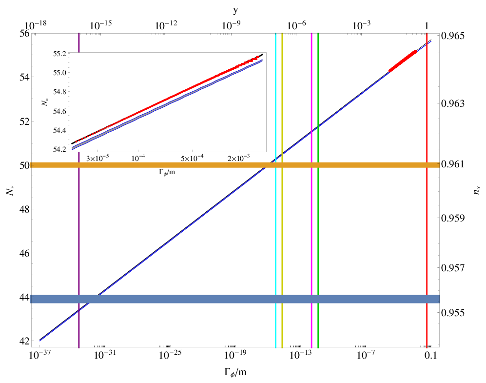
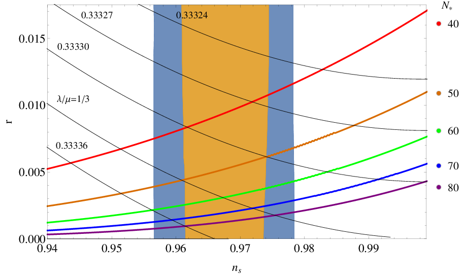
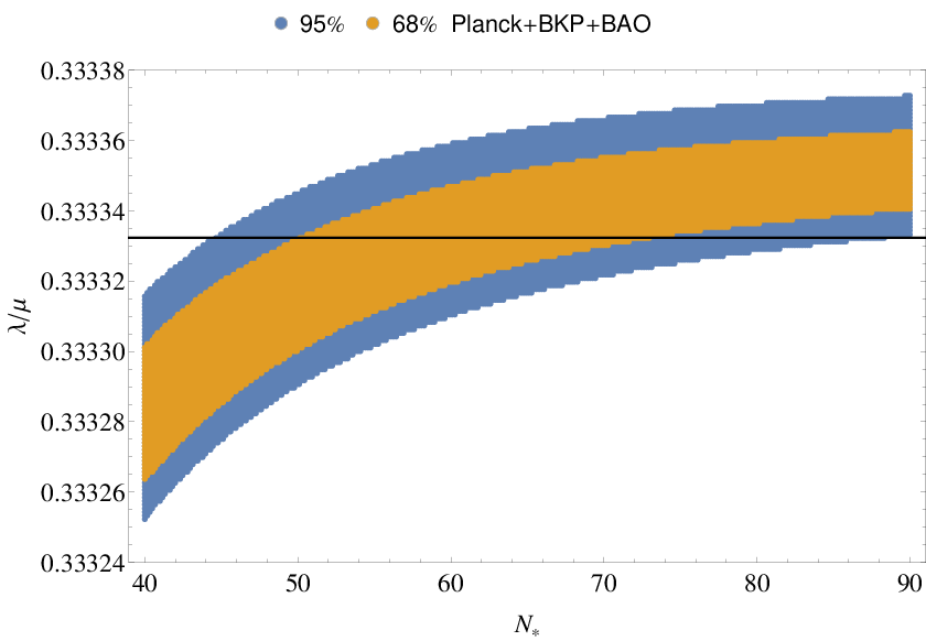
Fig. 6 confronts the Planck 2015 constraints [1] - the yellow shaded regions are favoured at the 68% CL and the blue shaded regions are allowed at the 95% CL - with the predictions of the simplest Wess-Zumino no-scale model [47] for different values of $N_{*}$ and $\lambda/\mu$ near the value 1/3 that reproduces Starobinsky-like predictions [69]. We see in the upper panel that the Planck 2015 constraints are almost independent of $r$ in the displayed range of $r$, and that the contours of fixed $N_{*}$ (coloured lines) intersect the contours of fixed $\lambda/\mu$ (black lines) at acute angles. Consequently, as seen in the lower panel, the Planck 2015 constraints on $N_{*}$ depend quite strongly on the value of $\lambda/\mu$. For the Starobinsky value $\lambda/\mu=1/3$ we find lower bounds

$$N_{*}\;\sim\;50\;\;(68\%~CL),\;\;\sim 44\;\;(95\%~CL)\,,$$

(45)

which are shown as horizontal yellow and blue lines, respectively, in Fig. 5. Their intersections with the diagonal blue line give the corresponding lower bounds on $\Gamma_{\phi}/m$ and $y$. We see that the lower bounds are already stronger than those imposed by successful Big Bang nucleosynthesis (vertical purple line) and the 68% CL lower limit approaches the upper limit on $y\sim 10^{-5}$ suggested by gravitino decays (vertical green line). Thus, the Planck data [1] already impose interesting constraints on inflaton decays in no-scale models: other examples are discussed in [69].

One of the biggest challenges in constructing models of inflation is to relate them to particle physics at accessible (collider) energies. One connection may be provided in principle by the discussion of inflaton decays in the previous section [58]. For example, in models where the inflaton is identified with the supersymmetric partner of a singlet (right-handed) neutrino in a see-saw model of neutrino masses, the constraints on the two-body decay coupling $y$ have potential implications for low-energy observables such as flavour-changing lepton transitions as well as scenarios for neutrino mixing. Another possible connection arises via supersymmetry breaking. For example, if the gauge kinetic function $f_{\alpha\beta}$ depends same non-trivially on the inflaton field $\phi$:

$$d_{g,\phi}\equiv\langle{\rm Re}\,f\rangle^{-1}\left|\left\langle\frac{\partial f}{\partial\phi}\right\rangle\right|\neq 0\,,$$

(46)

the inflaton decays into Standard Model gauge bosons and gauginos are given by [58]

$$\Gamma(\phi\rightarrow gg)=\Gamma(\phi\rightarrow\tilde{g}\tilde{g})=\frac{3d_{g,\phi}^{2}}{32\pi}\frac{m^{3}}{M_{P}^{2}}\,,$$

(47)

and the gaugino masses are given by

$$m_{1/2}={\cal O}(1)\times d_{g,\phi}\times m_{3/2}\,.$$

(48)

As already commented, the vertical yellow and magenta lines in Fig. 5 bracket the range of $y$ and hence $\Gamma_{\phi}/m$ found in Starobinsky-like no-scale models, which correspond to $N_{*}\in(50.5,51.5)$, with the upper end of this range corresponding to $d_{g,\phi}={\cal O}(1)$ and hence $m_{1/2}={\cal O}(m_{3/2})$.

Additionally, different assignments for the inflaton and matter fields lead to different possibilities for the pattern of supersymmetric particle masses, via their dependences on the model-dependent soft supersymmetry-breaking scalar masses $m_{0}$, gaugino masses $m_{1/2}$ and bilinear and trilinear scalar couplings $B_{0}$ and $A_{0}$ [58]. Among the possibilities are the original no-scale boundary conditions $m_{0}=B_{0}=A_{0}=0$ [39, 40], CMSSM-like boundary conditions in which $m_{0},B_{0}$ and $A_{0}$ are non-zero and universal for different scalar species and determined by the gravitino mass [31], mSUGRA-like boundary conditions in which $m_{0}+B_{0}=A_{0}$ [31, 73], etc. Thus, if supersymmetry is discovered and sparticle masses measured at accelerators, it may be possible constrain models of inflation, and vice versa if models of inflation can be constrained.

An example is given in Fig. 7, which displays results for a no-scale scenario with $m_{0}=B_{0}=A_{0}=0$ and $m_{1/2}\neq 0$ at some input renormalization scale $M_{in}$ in an SU(5) GUT model with superpotential terms $W\ni\lambda{H}{\Sigma}{\bar{H}}+(\lambda^{\prime}/6){\rm Tr}{\Sigma^{3}}$, where $H,{\bar{H}}$ and $\Sigma$ are $\mathbf{5},\mathbf{\bar{5}}$ and $\mathbf{24}$ Higgs representations, respectively, for the representative values $\lambda=-0.1,\lambda^{\prime}=2$ discussed in [74, 75]. We see that, within this particular model, only a restricted range of $m_{1/2}\in(800,1500)$ GeV is consistent with the LHC data. The relations (48, 47, 46) show how this type of constraint can then be applied to models of inflation and string compactification.

As we have reviewed in this article, no-scale supergravity is an attractive framework for constructing models of inflation, since supersymmetry accommodates naturally the required hierarchy between the scale of inflation and the Planck scale [16], gravity must be incorporated in any discussion of cosmology, and no-scale supergravity [38] emerges from generic string compactifications [42] and yields an effective potential that is positive semi-definite [43, 45]. We have discussed various no-scale inflationary scenarios, reviewing how they naturally yield an effective potential, and hence predictions for $n_{s}$ and $r$, that are coincident [47, 50] with the Planck-friendly Starobinsky model based on $R+R^{2}$ gravity [3]. Moreover, no-scale models achieve this in a technically natural way, via small superpotential couplings rather than surprisingly large non-minimal gravitational couplings as in the Starobinsky and Higgs inflation models.

The no-scale framework is, moreover, more flexible, being able to accommodate models intermediate between the Starobinsky model and a quadratic potential suitable for chaotic inflation [59, 63], which could yield larger values of $r$ that are still compatible with the constraints from Planck and other experiments. As in other supersymmetric models of inflation, it is necessary to take into account two-field effects: in the no-scale models we study [64], we find that these tend to reduce $r$ without generating large non-Gaussianity.

In principle, no-scale inflation could provide a phenomenological bridge between string theory and collider physics [58]. In addition to the above-mentioned model-dependence of $r$, the value of $n_{s}$ is related directly in Starobinsky-like models to the number of e-folds during inflation [69], which is in turn sensitive to the rate of inflaton decay and thereby the assignment of the inflaton as a modulus or matter field. The pattern of soft supersymmetry breaking is also sensitive to this assignment, and would be measurable at the LHC or in other collider experiments.

As we have mentioned, open issues in no-scale inflation include the mechanism for stabilization of the various moduli, including the volume modulus that plays a prominent rôle in building models. The inflationary observables are sensitive to the mechanism of modulus stabilization, and therefore may be able to cast some light on this basic issue in string phenomenology. More generally, for the foreseeable future measurements of inflationary observables are likely to take us closer to the string scale than any other experiments, and no-scale inflationary models may be the best platform for exploiting this scientific opportunity.

The work of J.E. was supported in part by the London Centre for Terauniverse Studies (LCTS), using funding from the European Research Council via the Advanced Investigator Grant 267352 and from the UK STFC via the research grant ST/L000326/1. The work of D.V.N. was supported in part by the DOE grant DE-FG03-95-ER-40917 and in part by the Alexander S. Onassis Public Benefit Foundation. The work of M.A.G.G. and K.A.O. was supported in part by DOE grant DE-SC0011842 at the University of Minnesota.

References

- [1] P. A. R. Ade et al. [Planck Collaboration], arXiv:1502.01589 [astro-ph.CO]; arXiv:1502.02114 [astro-ph.CO].
- [2] J. Martin, C. Ringeval and V. Vennin, Phys. Dark Univ. 5-6, 75-235 (2014) [arXiv:1303.3787 [astro-ph.CO]]; J. Martin, C. Ringeval, R. Trotta and V. Vennin, JCAP 1403 (2014) 039 [arXiv:1312.3529 [astro-ph.CO]]; J. Martin, arXiv:1502.05733 [astro-ph.CO].
- [3] A. A. Starobinsky, Phys. Lett. B 91, 99 (1980).
- [4] A. Ijjas, P. J. Steinhardt and A. Loeb, Phys. Lett. B 723 (2013) 261 [arXiv:1304.2785 [astro-ph.CO]]; J. L. Lehners and P. J. Steinhardt, Phys. Rev. D 87 (2013) 12, 123533 [arXiv:1304.3122 [astro-ph.CO]]; A. Ijjas, P. J. Steinhardt and A. Loeb, Phys. Lett. B 736 (2014) 142 [arXiv:1402.6980 [astro-ph.CO]].
- [5] G. Aad et al. [ATLAS Collaboration], Phys. Lett. B 716 (2012) 1 [arXiv:1207.7214 [hep-ex]]; S. Chatrchyan et al. [CMS Collaboration], Phys. Lett. B 716 (2012) 30 [arXiv:1207.7235 [hep-ex]].
- [6] F. L. Bezrukov and M. Shaposhnikov, Phys. Lett. B 659, 703 (2008) [arXiv:0710.3755 [hep-th]].
- [7] H. P. Nilles, Phys. Rept. 110 (1984) 1; H. E. Haber and G. L. Kane, Phys. Rept. 117 (1985) 75.
- [8] G. Aad et al. [ATLAS and CMS Collaborations], Phys. Rev. Lett. 114 (2015) 191803 [arXiv:1503.07589 [hep-ex]].
- [9] J. R. Ellis, G. Ridolfi and F. Zwirner, Phys. Lett. B 257 (1991) 83; H. E. Haber and R. Hempfling, Phys. Rev. Lett. 66 (1991) 1815; Y. Okada, M. Yamaguchi and T. Yanagida, Prog. Theor. Phys. 85 (1991) 1.
- [10] J. R. Ellis, S. Heinemeyer, K. A. Olive and G. Weiglein, Phys. Lett. B 515 (2001) 348 [hep-ph/0105061].
- [11] K. A. Olive, Phys. Rept. 190, 307 (1990).
- [12] A. D. Linde, Phys. Lett. B 108, 389 (1982); A. Albrecht and P. J. Steinhardt, Phys. Rev. Lett. 48, 1220 (1982).
- [13] A. Billoire and K. Tamvakis, Nucl. Phys. B 200, 329 (1982); J. D. Breit, S. Gupta and A. Zaks, Phys. Rev. Lett. 51, 1007 (1983).
- [14] A. D. Linde, Phys. Lett. B 116, 335 (1982).
- [15] W.H. Press, Phys. Scr. 21 (1980) 702; V.F. Mukhanov and G.V. Chibisov, JETP Lett. 33 (1981) 532; S.W. Hawking, Phys. Lett. 115B (1982) 295; A.A. Starobinsky, Phys. Lett. 117B (1982) 175; A.H. Guth and S.Y. Pi, Phys. Rev. Lett. 49 (1982) 1110; J.M. Bardeen, P.J. Steinhardt and M.S. Turner, Phys. Rev. D28 (1983) 679.
- [16] J. R. Ellis, D. V. Nanopoulos, K. A. Olive and K. Tamvakis, Phys. Lett. B 118 (1982) 335.
- [17] J. R. Ellis, D. V. Nanopoulos, K. A. Olive and K. Tamvakis, Nucl. Phys. B 221 (1983) 52.
- [18] J. R. Ellis, D. V. Nanopoulos, K. A. Olive and K. Tamvakis, Phys. Lett. B 120 (1983) 331.
- [19] K. Nakayama and F. Takahashi, JCAP 1110, 033 (2011) [arXiv:1108.0070 [hep-ph]].
- [20] G. D. Coughlan and G. G. Ross, Phys. Lett. B 157, 151 (1985); A. Albrecht and R. H. Brandenberger, Phys. Rev. D 31, 1225 (1985); L. G. Jensen and K. A. Olive, Phys. Lett. B 159, 99 (1985).
- [21] D. V. Nanopoulos, K. A. Olive and M. Srednicki, Phys. Lett. B 127, 30 (1983).
- [22] D. V. Nanopoulos, K. A. Olive, M. Srednicki and K. Tamvakis, Phys. Lett. B 123, 41 (1983).
- [23] A. B. Goncharov and A. D. Linde, Phys. Lett. B 139, 27 (1984).
- [24] E. Cremmer, S. Ferrara, L. Girardello and A. Van Proeyen, Nucl. Phys. B 212 (1983) 413.
- [25] R. Holman, P. Ramond and G. G. Ross, Phys. Lett. B 137, 343 (1984).
- [26] E. J. Copeland, A. R. Liddle, D. H. Lyth, E. D. Stewart and D. Wands, Phys. Rev. D 49, 6410 (1994) [astro-ph/9401011]; E. D. Stewart, Phys. Rev. D 51, 6847 (1995) [hep-ph/9405389].
- [27] G. D. Coughlan, W. Fischler, E. W. Kolb, S. Raby and G. G. Ross, Phys. Lett. B 131, 59 (1983); A. S. Goncharov, A. D. Linde and M. I. Vysotsky, Phys. Lett. B 147, 279 (1984); T. Banks, D. B. Kaplan and A. E. Nelson, Phys. Rev. D 49, 779 (1994) [hep-ph/9308292]; B. De Carlos, J. A. Casas, F. Quevedo, E. Roulet, Phys. Lett. B 318, 447 (1993) [hep-ph/9308325]; M. Kawasaki, T. Moroi and T. Yanagida Phys. Lett. B 370, 52 (1996) [hep-ph/9509399].
- [28] J. Ellis, D. V. Nanopoulos, and M. Quiros, Phys. Lett. B 174, 176 (1986);
- [29] T. Moroi, M. Yamaguchi and T. Yanagida Phys. Lett. B 342, 105 (1995) [hep-ph/9409367];
- [30] J. Polonyi, Budapest preprint KFKI-1977-93 (1977).
- [31] R. Barbieri, S. Ferrara and C. A. Savoy, Phys. Lett. B 119, 343 (1982).
- [32] I. Joichi and M. Yamaguchi, Phys. Lett. B 342, 111 (1995) [hep-ph/9409266];
- [33] M. Dine, R. Kitano, A. Morisse and Y. Shirman, Phys. Rev. D 73, 123518 (2006) [hep-ph/0604140]; R. Kitano, Phys. Lett. B 641, 203 (2006) [hep-ph/0607090]; R. Kallosh and A. D. Linde, JHEP 0702, 002 (2007) [hep-th/0611183]; H. Abe, T. Higaki and T. Kobayashi, Phys. Rev. D 76 (2007) 105003 [arXiv:0707.2671 [hep-th]]; J. Fan, M. Reece and L.-T. Wang, JHEP 1109, 126 (2011) [arXiv:1106.6044 [hep-ph]].
- [34] E. Dudas, C. Papineau and S. Pokorski, JHEP 0702, 028 (2007) [hep-th/0610297]; H. Abe, T. Higaki, T. Kobayashi and Y. Omura, Phys. Rev. D 75, 025019 (2007) [hep-th/0611024].
- [35] R. Kallosh, A. Linde, K. A. Olive and T. Rube, Phys. Rev. D 84, 083519 (2011) [arXiv:1106.6025 [hep-th]]; A. Linde, Y. Mambrini and K. A. Olive, Phys. Rev. D 85, 066005 (2012) [arXiv:1111.1465 [hep-th]]; E. Dudas, A. Linde, Y. Mambrini, A. Mustafayev and K. A. Olive, arXiv:1209.0499 [hep-ph].
- [36] J. L. Evans, M. A. G. Garcia and K. A. Olive, JCAP 1403, 022 (2014) [arXiv:1311.0052 [hep-ph]].
- [37] M. K. Gaillard, H. Murayama and K. A. Olive, Phys. Lett. B 355 (1995) 71 [hep-ph/9504307].
- [38] E. Cremmer, S. Ferrara, C. Kounnas and D. V. Nanopoulos, Phys. Lett. B 133 (1983) 61; J. R. Ellis, A. B. Lahanas, D. V. Nanopoulos and K. Tamvakis, Phys. Lett. B 134 (1984) 429.
- [39] A. B. Lahanas and D. V. Nanopoulos, Phys. Rept. 145 (1987) 1.
- [40] J. R. Ellis, C. Kounnas and D. V. Nanopoulos, Nucl. Phys. B 247 (1984) 373.
- [41] M. Kawasaki, M. Yamaguchi and T. Yanagida, Phys. Rev. Lett. 85, 3572 (2000) [arXiv:hep-ph/0004243].
- [42] E. Witten, Phys. Lett. B 155 (1985) 151; see also S. B. Giddings, S. Kachru and J. Polchinski, Phys. Rev. D 66, 106006 (2002) [hep-th/0105097]; V. Balasubramanian, P. Berglund, J. P. Conlon and F. Quevedo, JHEP 0503, 007 (2005) [hep-th/0502058].
- [43] A. S. Goncharov and A. D. Linde, Class. Quant. Grav. 1, L75 (1984).
- [44] C. Kounnas and M. Quiros, Phys. Lett. B 151, 189 (1985).
- [45] J. R. Ellis, K. Enqvist, D. V. Nanopoulos, K. A. Olive and M. Srednicki, Phys. Lett. B 152 (1985) 175 [Erratum-ibid. 156B (1985) 452].
- [46] K. Enqvist, D. V. Nanopoulos and M. Quiros, Phys. Lett. B 159, 249 (1985); P. Binétruy and M. K. Gaillard, Phys. Rev. D 34, 3069 (1986); H. Murayama, H. Suzuki, T. Yanagida and J. Yokoyama, Phys. Rev. D 50, 2356 (1994) [arXiv:hep-ph/9311326]; S. C. Davis and M. Postma, JCAP 0803, 015 (2008) [arXiv:0801.4696 [hep-ph]]; S. Antusch, M. Bastero-Gil, K. Dutta, S. F. King and P. M. Kostka, JCAP 0901, 040 (2009) [arXiv:0808.2425 [hep-ph]]; S. Antusch, M. Bastero-Gil, K. Dutta, S. F. King and P. M. Kostka, Phys. Lett. B 679, 428 (2009) [arXiv:0905.0905 [hep-th]]; S. Antusch, K. Dutta, J. Erdmenger and S. Halter, JHEP 1104 (2011) 065 [arXiv:1102.0093 [hep-th]]; R. Kallosh and A. Linde, JCAP 1011, 011 (2010) [arXiv:1008.3375 [hep-th]]; R. Kallosh, A. Linde and T. Rube, Phys. Rev. D 83, 043507 (2011) [arXiv:1011.5945 [hep-th]]; T. Li, Z. Li and D. V. Nanopoulos, JCAP 1402, 028 (2014) [arXiv:1311.6770 [hep-ph]]; W. Buchmuller, C. Wieck and M. W. Winkler, Phys. Lett. B 736, 237 (2014) [arXiv:1404.2275 [hep-th]].
- [47] J. Ellis, D. V. Nanopoulos and K. A. Olive, Phys. Rev. Lett. 111 (2013) 111301 [Phys. Rev. Lett. 111 (2013) 12, 129902] [arXiv:1305.1247 [hep-th]].
- [48] P. A. R. Ade et al. [Planck Collaboration], Astron. Astrophys. 571 (2014) A16 [arXiv:1303.5076 [astro-ph.CO]]; Astron. Astrophys. 571 (2014) A22 [arXiv:1303.5082 [astro-ph.CO]].
- [49] D. Croon, J. Ellis and N. E. Mavromatos, Phys. Lett. B 724 (2013) 165 [arXiv:1303.6253 [astro-ph.CO]].
- [50] J. Ellis, D. V. Nanopoulos and K. A. Olive, JCAP 1310 (2013) 009 [arXiv:1307.3537].
- [51] J. Ellis, H. J. He and Z. Z. Xianyu, Phys. Rev. D 91 (2015) 2, 021302 [arXiv:1411.5537 [hep-ph]].
- [52] P. A. R. Ade et al. [BICEP2 and Planck Collaborations], Phys. Rev. Lett. 114, no. 10, 101301 (2015) [arXiv:1502.00612 [astro-ph.CO]].
- [53] S. Ferrara, A. Kehagias and A. Riotto, Fortsch. Phys. 62, 573 (2014) [arXiv:1403.5531 [hep-th]]; S. Ferrara, A. Kehagias and A. Riotto, Fortsch. Phys. 63, 2 (2015) [arXiv:1405.2353 [hep-th]]; R. Kallosh, A. Linde, B. Vercnocke and W. Chemissany, JCAP 1407, 053 (2014) [arXiv:1403.7189 [hep-th]]; K. Hamaguchi, T. Moroi and T. Terada, Phys. Lett. B 733, 305 (2014) [arXiv:1403.7521 [hep-ph]].
- [54] Unfortunately, we do not have space in this summary to do justice to the extensive recent literature following [47]. See, for example: R. Kallosh and A. Linde, JCAP 1306 (2013) 028 [arXiv:1306.3214 [hep-th]]; T. Li, Z. Li and D. V. Nanopoulos, JCAP 1404, 018 (2014) [arXiv:1310.3331 [hep-ph]]; T. Li, Z. Li and D. V. Nanopoulos, Eur. Phys. J. C 75, no. 2, 55 (2015) [arXiv:1405.0197 [hep-th]]; C. P. Burgess, M. Cicoli and F. Quevedo, JCAP 1311 (2013) 003 [arXiv:1306.3512 [hep-th]]; F. Farakos, A. Kehagias and A. Riotto, Nucl. Phys. B 876, 187 (2013) [arXiv:1307.1137 [hep-th]]; S. Ferrara, R. Kallosh, A. Linde and M. Porrati, Phys. Rev. D 88 (2013) 8, 085038 [arXiv:1307.7696 [hep-th]]; W. Buchmüller, V. Domcke and C. Wieck, Phys. Lett. B 730, 155 (2014) [arXiv:1309.3122 [hep-th]]; C. Pallis, JCAP 1404, 024 (2014) [arXiv:1312.3623 [hep-ph]]; C. Pallis, JCAP 1408, 057 (2014) [arXiv:1403.5486 [hep-ph]]; I. Antoniadis, E. Dudas, S. Ferrara and A. Sagnotti, Phys. Lett. B 733, 32 (2014) [arXiv:1403.3269 [hep-th]]; W. Buchmuller, E. Dudas, L. Heurtier and C. Wieck, JHEP 1409, 053 (2014) [arXiv:1407.0253 [hep-th]]; C. Kounnas, D. Lüst and N. Toumbas, Fortsch. Phys. 63, 12 (2015) [arXiv:1409.7076 [hep-th]]; T. Terada, Y. Watanabe, Y. Yamada and J. Yokoyama, JHEP 1502, 105 (2015) [arXiv:1411.6746 [hep-ph]]; A. B. Lahanas and K. Tamvakis, Phys. Rev. D 91, no. 8, 085001 (2015) [arXiv:1501.06547 [hep-th]]; I. Dalianis and F. Farakos, arXiv:1502.01246 [gr-qc]; D. Roest and M. Scalisi, arXiv:1503.07909 [hep-th]; M. Scalisi, arXiv:1506.01368 [hep-th].
- [55] B. Whitt, Phys. Lett. B 145 (1984) 176.
- [56] V. F. Mukhanov and G. V. Chibisov, JETP Lett. 33, 532 (1981) [Pisma Zh. Eksp. Teor. Fiz. 33, 549 (1981)]; A. A. Starobinsky, Sov. Astron. Lett. 9, 302 (1983).
- [57] S. Cecotti, Phys. Lett. B 190 (1987) 86.
- [58] J. Ellis, M. A. G. Garcia, D. V. Nanopoulos and K. A. Olive, arXiv:1503.08867 [hep-ph].
- [59] J. Ellis, M. A. G. García, D. V. Nanopoulos and K. A. Olive, JCAP 1405 (2014) 037 [arXiv:1403.7518 [hep-ph]].
- [60] J. R. Ellis, C. Kounnas and D. V. Nanopoulos, Phys. Lett. B 143, 410 (1984).
- [61] S. Kachru, R. Kallosh, A. D. Linde and S. P. Trivedi, Phys. Rev. D 68, 046005 (2003) [arXiv:hep-th/0301240]; R. Kallosh and A. D. Linde, JHEP 0412, 004 (2004) [arXiv:hep-th/0411011]; R. Kallosh and A. D. Linde, JCAP 0704, 017 (2007) [arXiv:0704.0647 [hep-th]].
- [62] E. Dudas and C. Wieck, arXiv:1506.01253 [hep-th].
- [63] J. Ellis, M. A. G. Garcia, D. V. Nanopoulos and K. A. Olive, JCAP 1408 (2014) 044 [arXiv:1405.0271 [hep-ph]].
- [64] J. Ellis, M. A. G. García, D. V. Nanopoulos and K. A. Olive, JCAP 1501 (2015) 01, 010 [arXiv:1409.8197 [hep-ph]].
- [65] L. J. Dixon, V. Kaplunovsky and J. Louis, Nucl. Phys. B 329 (1990) 27; J. A. Casas, in Proceedings, International Europhysics Conference on High-Energy Physics, Jerusalem, Israel, August 19-25, 1997, eds. D. Lellouch, G. Mikenberg and E. Rabinovici, pp 914-917 [hep-ph/9802210].
- [66] C. Gordon, D. Wands, B. A. Bassett and R. Maartens, Phys. Rev. D 63, 023506 (2001) [astro-ph/0009131]; C. T. Byrnes and D. Wands, Phys. Rev. D 74, 043529 (2006) [astro-ph/0605679]; R. Easther, J. Frazer, H. V. Peiris and L. C. Price, Phys. Rev. Lett. 112 (2014) 161302 [arXiv:1312.4035 [astro-ph.CO]].
- [67] S. Renaux-Petel and K. Turzynski, JCAP 1506 (2015) 06, 010 [arXiv:1405.6195 [astro-ph.CO]].
- [68] P. A. R. Ade et al. [Planck Collaboration], arXiv:1502.01592 [astro-ph.CO].
- [69] J. Ellis, M. A. G. Garcia, D. V. Nanopoulos and K. A. Olive, arXiv:1505.06986 [hep-ph].
- [70] A. R. Liddle and S. M. Leach, Phys. Rev. D 68, 103503 (2003) [astro-ph/0305263].
- [71] K. Dutta and A. Maharana, Phys. Rev. D 91 (2015) 4, 043503 [arXiv:1409.7037 [hep-ph]]; K. Das, K. Dutta and A. Maharana, arXiv:1506.05745 [hep-ph].
- [72] M. Bolz, A. Brandenburg and W. Buchmuller, Nucl. Phys. B 606, 518 (2001) [Erratum-ibid. B 790, 336 (2008)] [hep-ph/0012052]; R. H. Cyburt, J. Ellis, B. D. Fields and K. A. Olive, Phys. Rev. D 67, 103521 (2003) [astro-ph/0211258]; F. D. Steffen, JCAP 0609, 001 (2006) [hep-ph/0605306]; M. Kawasaki, K. Kohri, T Moroi and A.Yotsuyanagi, Phys. Rev. D 78, 065011 (2008) [arXiv:0804.3745 [hep-ph]]; R. H. Cyburt, J. Ellis, B. D. Fields, F. Luo, K. A. Olive and V. C. Spanos, JCAP 0910, 021 (2009) [arXiv:0907.5003 [astro-ph.CO]]; R. H. Cyburt, J. Ellis, B. D. Fields, F. Luo, K. A. Olive and V. C. Spanos, JCAP 1305, 014 (2013) [arXiv:1303.0574 [astro-ph.CO]].
- [73] J. R. Ellis, K. A. Olive, Y. Santoso and V. C. Spanos, Phys. Lett. B 573 (2003) 162 [arXiv:hep-ph/0305212], and Phys. Rev. D 70 (2004) 055005 [arXiv:hep-ph/0405110].
- [74] J. Ellis, A. Mustafayev and K. A. Olive, Eur. Phys. J. C 69, 219 (2010) [arXiv:1004.5399 [hep-ph]].
- [75] J. Ellis, D. V. Nanopoulos and K. A. Olive, Phys. Rev. D 89 (2014) 4, 043502 [arXiv:1310.4770 [hep-ph]].
- [76] T. Hahn, S. Heinemeyer, W. Hollik, H. Rzehak and G. Weiglein, Phys. Rev. Lett. 112 (2014) 14, 141801 [arXiv:1312.4937 [hep-ph]].