The asymptotic behavior of the minimal pseudo-Anosov dilatations in the hyperelliptic handlebody groupsThanks: The first author is supported by Grant-in-Aid for Scientific Research (C) (No. 16K05156), Japan Society for the Promotion of Science. The second author is supported by Grant-in-Aid for Scientific Research (C) (No. 15K04875), Japan Society for the Promotion of Science.

Susumu Hirose Address: Department of Mathematics, Faculty of Science and Technology, Tokyo University of Science, Noda, Chiba, 278-8510, Japan Email address: hirose_susumu@ma.noda.tus.ac.jp and Eiko Kin Address: Department of Mathematics, Graduate School of Science, Osaka University Toyonaka, Osaka 560-0043, JAPAN Email address: kin@math.sci.osaka-u.ac.jp

Date: August 24, 2026

Abstract.

We consider the hyperelliptic handlebody group on a closed surface of genus $g$ . This is the subgroup of the mapping class group on a closed surface of genus $g$ consisting of isotopy classes of homeomorphisms on the surface that commute with some fixed hyperelliptic involution and that extend to homeomorphisms on the handlebody. We prove that the logarithm of the minimal dilatation (i.e, the minimal entropy) of all pseudo-Anosov elements in the hyperelliptic handlebody group of genus $g$ is comparable to $1/g$ . This means that the asymptotic behavior of the minimal pseudo-Anosov dilatation of the subgroup of genus $g$ in question is the same as that of the ambient mapping class group of genus $g$ . We also determine finite presentations of the hyperelliptic handlebody groups.

Key words and phrases:

pseudo-Anosov, dilatation, handlebody group, hyperelliptic mapping class group, Hilden group, wicket group

2000 Mathematics Subject Classification

Primary 57M27, 37E30, Secondary 37B40

1. Introduction

Let $\varSigma_{g}$ be a closed, orientable surface of genus $g$ , and let $\mathrm{Mod}(\varSigma_{g})$ be the mapping class group on $\varSigma_{g}$ . The hyperelliptic mapping class group $\mathcal{H}(\varSigma_{g})$ is the subgroup of $\mathrm{Mod}(\varSigma_{g})$ consisting of isotopy classes of orientation preserving homeomorphisms on $\varSigma_{g}$ that commute with some fixed hyperelliptic involution $\mathcal{S}:\varSigma_{g}\rightarrow\varSigma_{g}$ . If $g\geq 3$ , then $\mathcal{H}(\varSigma_{g})$ is of infinite index in $\mathrm{Mod}(\varSigma_{g})$ , and it is a particular subgroup in some sense. Despite such a property, $\mathcal{H}(\varSigma_{g})$ plays a significant role to study the mapping class group $\mathrm{Mod}(\varSigma_{g})$ . Especially, elements of $\mathcal{H}(\varSigma_{g})$ have a handy description via the spherical braid group $SB_{2g+2}$ with $2g+2$ strings, which is proved by Birman-Hilden:

\mathcal{H}(\varSigma_{g})/\langle\iota\rangle\simeq SB_{2g+2}/\langle\Delta^{2}\rangle,

where $\iota=[\mathcal{S}]\in\mathcal{H}(\varSigma_{g})$ is the mapping class of $\mathcal{S}$ , and $\Delta\in SB_{2g+2}$ is a half twist braid. Here $\langle\iota\rangle$ and $\langle\Delta^{2}\rangle$ are the subgroups generated by $\iota$ and $\Delta^{2}$ respectively. There exists a natural surjective homomorphism from $SB_{2g+2}$ to the mapping class group $\mathrm{Mod}(\varSigma_{0,2g+2})$ on a sphere with $2g+2$ punctures:

\Gamma:SB_{2g+2}\rightarrow\mathrm{Mod}(\varSigma_{0,2g+2})

with the kernel generated by $\Delta^{2}$ .

Let $G$ be a subgroup of $\mathrm{Mod}(\varSigma_{g})$ . Whenever $G\cap\mathcal{H}(\varSigma_{g})$ contains a non-trivial element, it is worthwhile to consider the subgroup $G\cap\mathcal{H}(\varSigma_{g})$ of $\mathrm{Mod}(\varSigma_{g})$ . The group $G\cap\mathcal{H}(\varSigma_{g})$ would be an intriguing one in its own right. Also we may have a chance to find new examples or phenomena on $G$ by using a handy braid description of $G\cap\mathcal{H}(\varSigma_{g})$ . In the case $G$ is the Torelli group $\mathcal{I}(\varSigma_{g})$ consisting of elements of $\mathrm{Mod}(\varSigma_{g})$ which act trivially on $H_{1}(\varSigma_{g};{\mathbb{Z}})$ , the hyperelliptic Torelli group $\mathcal{I}(\varSigma_{g})\cap\mathcal{H}(\varSigma_{g})$ is studied by Brendle-Margalit, see [6] and references therein. In this paper, we consider the handlebody group $\mathrm{Mod}({\mathbb{H}}_{g})$ as $G$ . This is the subgroup of $\mathrm{Mod}(\varSigma_{g})$ consisting of isotopy classes of orientation preserving homeomorphisms on $\varSigma_{g}$ that extend to homeomorphisms on the handlebody ${\mathbb{H}}_{g}$ of genus $g$ . The main subgroup of $\mathrm{Mod}(\varSigma_{g})$ in this paper is the hyperelliptic handlebody group

\mathcal{H}({\mathbb{H}}_{g})=\mathrm{Mod}({\mathbb{H}}_{g})\cap\mathcal{H}(\varSigma_{g}).

We prove a version of Birman-Hilden’s theorem about $\mathcal{H}({\mathbb{H}}_{g})$ , and identify the subgroup of $SB_{2g+2}$ corresponding to $\mathcal{H}({\mathbb{H}}_{g})$ . More precisely, we prove in Theorem 2.11 that

\mathcal{H}({\mathbb{H}}_{g})/\langle\iota\rangle\simeq SW_{2g+2}/\langle\Delta^{2}\rangle,

where $SW_{2g+2}$ is so called the wicket group. (See Section 2.5.1.) Hilden introduced a subgroup $SH_{2g+2}$ of $\mathrm{Mod}(\varSigma_{0,2g+2})$ in [15], which is now called the (spherical) Hilden group. The group $SH_{2g+2}$ is isomorphic to the image $\Gamma(SW_{2g+2})$ under $\Gamma:SB_{2g+2}\rightarrow\mathrm{Mod}(\varSigma_{0,2g+2})$ (Theorem 2.6). As an application of the above relation between $\mathcal{H}({\mathbb{H}}_{g})$ and $SW_{2g+2}$ , we determine a finite presentation of $\mathcal{H}({\mathbb{H}}_{g})$ in Appendix A, see Theorem A.8

We are interested in the asymptotic behavior of the minimal dilatations of all pseudo-Anosov elements in $\mathcal{H}({\mathbb{H}}_{g})$ varying $g$ . To state our results, we need some setup. Let $\varSigma$ be an orientable, connected surface possibly with punctures. A homeomorphism $\Phi:\varSigma\rightarrow\varSigma$ is pseudo-Anosov if there exist a pair of transverse measured foliations $(\mathcal{F}^{u},\mu^{u})$ and $(\mathcal{F}^{s},\mu^{s})$ and a constant $\lambda=\lambda(\Phi)>1$ such that

\Phi(\mathcal{F}^{u},\mu^{u})=(\mathcal{F}^{u},\lambda\mu^{u})\ \hskip 5.69054pt\mbox{and}\ \hskip 5.69054pt\Phi(\mathcal{F}^{s},\mu^{s})=(\mathcal{F}^{s},\lambda^{-1}\mu^{s}).

Then $\mathcal{F}^{u}$ and $\mathcal{F}^{s}$ are called the unstable and stable foliations, and $\lambda$ is called the dilatation or stretch factor of $\Phi$ . The topological entropy $\mathrm{ent}(\Phi)$ is precisely equal to $\log\lambda(\Phi)$ . A significant property of pseudo-Anosov homeomorphisms is that $\mathrm{ent}(\Phi)$ attains the minimal entropy among all homeomorphisms on $\varSigma$ which are isotopic to $\Phi$ , see [11, Exposé 10]. An element $\phi$ of the mapping class group $\mathrm{Mod}(\varSigma)$ of $\varSigma$ is called pseudo-Anosov if $\phi$ contains a pseudo-Anosov homeomorphism $\Phi:\varSigma\rightarrow\varSigma$ as a representative. In this case, we let $\lambda(\phi)=\lambda(\Phi)$ and $\mathrm{ent}(\phi)=\mathrm{ent}(\Phi)$ , and we call them the dilatation and entropy of $\phi$ respectively. We call

\mathrm{Ent}(\phi)=|\chi(\varSigma)|\mathrm{ent}(\phi)

the normalized entropy of $\phi$ , where $\chi(\varSigma)$ is the Euler characteristic of $\varSigma$ .

Let $f:\varSigma\rightarrow\varSigma$ be a representative of a given mapping class $\phi\in\mathrm{Mod}(\varSigma)$ . The mapping torus ${\mathbb{T}}_{\phi}={\mathbb{T}}_{[f]}$ is defined by

{\mathbb{T}}_{\phi}=\varSigma\times{\mathbb{R}}/\sim,

where $\sim$ identifies $(x,t+1)$ with $(f(x),t)$ for $x\in\varSigma$ and $t\in{\mathbb{R}}$ . We call $\phi$ the monodromy of ${\mathbb{T}}_{\phi}$ . We sometimes call the representative $f\in\phi$ the monodromy of ${\mathbb{T}}_{\phi}$ . The suspension flow $f^{t}$ on ${\mathbb{T}}_{\phi}$ is a flow induced by the vector field $\tfrac{\partial}{\partial t}$ . The hyperbolization theorem by Thurston [33] states that when a $3$ -manifold $M$ is a surface bundle over the circle, that is $M\simeq{\mathbb{T}}_{\phi}$ for some mapping class $\phi$ , $M$ admits a hyperbolic structure if and only if $\phi$ is pseudo-Anosov.

We fix a surface $\varSigma$ , and consider the set of dilatations of all pseudo-Anosov elements on $\varSigma$ :

\mathrm{dil}(\varSigma)=\{\lambda(\phi)\ |\ \phi\in\mathrm{Mod}(\varSigma)\ \mbox{is pseudo-Anosov}\}.

This is a closed, discrete subset of ${\mathbb{R}}$ , see [20] for example. In particular, given a subgroup $G$ of $\mathrm{Mod}(\varSigma)$ which contains pseudo-Anosov elements, there exists a minimum $\delta(G)>1$ among dilatations of all pseudo-Anosov elements in $G$ . Clearly we have $\delta(G)\geq\delta(\mathrm{Mod}(\varSigma))$ . Let $\varSigma_{g,n}$ be a closed, orientable surface of genus $g$ removed $n$ punctures. We denote by $\delta_{g}$ and $\delta_{g,n}$ , the minimal dilatations $\delta(\mathrm{Mod}(\varSigma_{g}))$ and $\delta(\mathrm{Mod}(\varSigma_{g,n}))$ respectively.

By pioneering work of Penner [27], the asymptotic equality

\log\delta_{g}\asymp\tfrac{1}{g}

holds. Here $A\asymp B$ means that there exists a universal constant $c>0$ so that $\tfrac{A}{c}<B<cA$ . In this case, we say that $A$ is comparable to $B$ . Penner proves this claim by using his lower bound $\log\delta_{g,n}\geq\tfrac{\log 2}{12g+4n-12}$ ([27]). After work of Penner, one can ask the following.

Question 1.1.

Which sequence of subgroups $G_{(g)}$ ’s of $\mathrm{Mod}(\varSigma_{g})$ satisfies $\log\delta(G_{(g)})\asymp\tfrac{1}{g}$ ?

Hironaka also studied Question 1.1 in [16]. To prove $\log\delta(G_{(g)})\asymp\tfrac{1}{g}$ , thanks to the Penner’s lower bound $\log\delta_{g}\geq\tfrac{\log 2}{12g-12}$ , it suffices to construct a sequence of pseudo-Anosov elements $\phi_{(g)}\in G_{(g)}$ for $g\geq 2$ whose normalized entropies $\mathrm{Ent}(\phi_{(g)})=(2g-2)\mathrm{ent}(\phi_{(g)})$ are uniformly bounded from above.

It is a result by Farb-Leininger-Margalit that the dilatation of any pseudo-Anosov element in the Torelli group $\mathcal{I}(\varSigma_{g})$ has a uniform lower bound ([9, Theorem 1.1]). See also Agol-Leininger-Margalit [1]. On the other hand, the two subgroups $\mathcal{H}(\varSigma_{g})$ and $\mathrm{Mod}({\mathbb{H}}_{g})$ are examples of answers to Question 1.1. In fact, Hironaka-Kin prove in [18, Theorem 1.1],

g\log\delta(\mathcal{H}(\varSigma_{g}))<\log(2+\sqrt{3})\approx 1.3169\hskip 5.69054pt\mbox{for}\ g\geq 2.

Hironaka proves in [16, Section 3.1],

(1.1)

\limsup_{g\to\infty}g\log\delta(\mathrm{Mod}({\mathbb{H}}_{g}))\leq\log(33+8\sqrt{17})\approx 4.1894.

The main result of this paper is to prove that $\log\delta(\mathcal{H}({\mathbb{H}}_{g}))$ is still comparable to $1/g$ .

Theorem 1.2.

We have $\log\delta(\mathcal{H}({\mathbb{H}}_{g}))\asymp\frac{1}{g}$ and $\log\delta(SH_{2n})\asymp\frac{1}{n}$ .

Proposition 1.3.

There exists a sequence of pseudo-Anosov braids $w_{2n}\in SW_{2n}$ $(n\geq 3)$ such that

\displaystyle\lim_{n\to\infty}n\log(\lambda(w_{2n}))=2\log\kappa,

where $\kappa=\tfrac{1+\sqrt{5}}{2}+\tfrac{\sqrt{2+2\sqrt{5}}}{2}\approx 2.89005$ equals the largest root of

t^{4}-2t^{3}-2t^{2}-2t+1=(t^{2}-(1+\sqrt{5})t+1)(t^{2}-(1-\sqrt{5})t+1).

The braids $w_{2n}$ ’s are written by the standard generators of the spherical braid groups concretely (Section 3). Theorem 1.2 follows from Proposition 1.3 as we explain now. We say that a braid $b\in SB_{2g+2}$ is pseudo-Anosov if $\Gamma(b)\in\mathrm{Mod}(\varSigma_{0,2g+2})$ is a pseudo-Anosov mapping class. In this case, the dilatation $\lambda(b)$ is defined by the dilatation $\lambda(\Gamma(b))$ of the pseudo-Anosov element $\Gamma(b)$ . On the other hand, there exists a surjective homomorphism $Q:\mathcal{H}({\mathbb{H}}_{g})\rightarrow SH_{2g+2}$ with the kernel $\langle\iota\rangle$ (Theorem 2.11). If $\phi\in\mathcal{H}({\mathbb{H}}_{g})$ is pseudo-Anosov, then $Q(\phi)\in SH_{2g+2}$ is also pseudo-Anosov. If $\Phi:\varSigma_{0,2g+2}\rightarrow\varSigma_{0,2g+2}$ is a pseudo-Anosov homeomorphism which represents $Q(\phi)$ , then one can take a pseudo-Anosov homeomoprhism $\tilde{\Phi}:\varSigma_{g}\rightarrow\varSigma_{g}$ which is a lift of $\Phi$ such that $\phi=[\tilde{\Phi}]$ . Two pseudo-Anosov homeomorphisms $\Phi$ and $\tilde{\Phi}$ have the same dilatation, since their local dynamics are the same. Hence we have $\lambda(\phi)=\lambda(Q(\phi))$ . In particular we have $\delta(\mathcal{H}({\mathbb{H}}_{g}))=\delta(SH_{2g+2})$ for $g\geq 2$ (Lemma 2.12). Proposition 1.3 says that there exists a sequence of pseudo-Anosov elements $\Gamma(w_{2n})\in SH_{2n}$ whose normalized entropies $\mathrm{Ent}(\Gamma(w_{2n}))$ are uniformly bounded from above. Thus the same thing occurs in $\mathcal{H}({\mathbb{H}}_{g})$ . See Section 2.6.

By Proposition 1.3 together with $\delta(\mathcal{H}({\mathbb{H}}_{g}))=\delta(SH_{2g+2})$ , the following holds.

Theorem 1.4.

We have $\displaystyle\limsup_{g\to\infty}g\log\delta(\mathcal{H}({\mathbb{H}}_{g}))\leq 2\log\kappa\approx 2.12255$ .

Since $\mathcal{H}({\mathbb{H}}_{g})$ is the subgroup of $\mathrm{Mod}({\mathbb{H}}_{g})$ , we have $\delta(\mathrm{Mod}({\mathbb{H}}_{g}))\leq\delta(\mathcal{H}({\mathbb{H}}_{g}))$ . Comparing Theorem 1.4 with (1.1), we find that Theorem 1.4 improves the previous upper bound of $\delta(\mathrm{Mod}({\mathbb{H}}_{g}))$ by Hironaka. In this sense, the sequence of pseudo-Anosov elements of $\mathcal{H}({\mathbb{H}}_{g})$ used for the proof of Theorem 1.4 is a new example for $\mathrm{Mod}({\mathbb{H}}_{g})$ whose normalized entropies are uniformly bounded from above.

Let us mention a property of the sequence of pseudo-Anosov braids $w_{2n}$ ’s in Proposition 1.3 and give an outline of its proof. (See Section 3 for more details.) Let $L_{0}$ be a link with $3$ components as in Figure 1. The mapping torus of $\Gamma(w_{6})\in\mathrm{Mod}(\varSigma_{0,6})$ is homeomorphic to $S^{3}\setminus L_{0}$ , that is the complement of $L_{0}$ in a $3$ -sphere $S^{3}$ . Thus once we prove that $w_{6}$ is a pseudo-Anosov braid, it follows that $S^{3}\setminus L_{0}$ is a hyperbolic fibered $3$ -manifold. The sequence $w_{8},w_{10},w_{12},\cdots$ has a property such that if $k=4n+8$ , then the mapping torus of $\Gamma(w_{k})$ is homeomorphic to $S^{3}\setminus L_{0}$ , and if $k=4n+6$ , then the fibration of the mapping torus of $\Gamma(w_{k})$ comes from a fibration of $S^{3}\setminus L_{0}$ by Dehn filling cusps along the boundary slopes of a fiber (which depends on $k$ ). A technique about disk twists (see Section 2.7) provides a method of constructing sequences of mapping classes on punctured spheres whose mapping tori are homeomorphic to each other. We use this technique for the construction of the sequence $w_{8},w_{12},\cdots,w_{4n+8},\cdots$ from the mapping torus of $\Gamma(w_{6})$ . We conclude that the braids $w_{8},w_{12},\cdots,w_{4n+8},\cdots$ are pseudo-Anosov from the fact that $S^{3}\setminus L_{0}$ is hyperbolic. We point out that our method by using disk twists quite suit to construct elements in the Hilden groups whose mapping tori are homeomorphic to each other. Now let $\Phi=\Phi_{6}:\varSigma_{0,6}\rightarrow\varSigma_{0,6}$ be the pseudo-Anosov homeomorphism which represents $\Gamma(w_{6})$ , and let $\tau_{6}$ and $\mathfrak{p}_{6}:\tau_{6}\rightarrow\tau_{6}$ be the invariant train track and the train track representative for $\Gamma(w_{6})$ respectively. We find that $\lambda(w_{6})$ is equal to the constant $\kappa$ in Proposition 1.3. An analysis by using the suspension flow $\Phi^{t}$ on $S^{3}\setminus L_{0}$ and the train track representative $\mathfrak{p}_{6}:\tau_{6}\rightarrow\tau_{6}$ tells us the dynamics of the pseudo-Anosov homeomorphism which represents $\Gamma(w_{4n+8})$ for each $n\geq 0$ . In particular one can construct the train track representative $\mathfrak{p}_{4n+8}:\tau_{4n+8}\rightarrow\tau_{4n+8}$ for $\Gamma(w_{4n+8})$ concretely. From the ‘shape’ of the invariant train track $\tau_{4n+8}$ , we see that $w_{4n+6}$ is a pseudo-Anosov braid with the same dilatation as $w_{4n+8}$ . By a study of a particular fibered face for the exterior of the link $L_{0}$ , we see that the normalized entropy of $\Gamma(w_{4n+8})$ converges to the one of $\Gamma(w_{6})$ , which implies that Proposition 1.3 holds.

From view point of fibered faces of fibered $3$ -manifolds, the sequence of mapping classes $\Gamma(w_{4n+8})$ ’s are obtained from a certain deformation of the monodromy $\Gamma(w_{6})$ on the $\varSigma_{0,6}$ -fiber of the fibration on $S^{3}\setminus L_{0}$ . See also Hironaka [17] and Valdivia [34] for other constructions in which fibered faces on hyperbolic $3$ -manifolds are used crucially.

Refer to caption — Figure 1. Link $L_{0}$ which gets the name $L10n95$ in the Thistlethwaite link table, see the Knot Atlas [22].

By using Penner’s lower bound $\log\delta_{0,n}\geq\tfrac{\log 2}{4n-12}$ , Hironaka-Kin prove that $\log\delta_{0,n}\asymp\tfrac{1}{n}$ ([18]). In fact, it is shown in [18] that the subgroup $\Gamma(SB_{(n-1)})$ of $\mathrm{Mod}(\varSigma_{0,n})$ which consists of all mapping classes on an $(n-1)$ -punctured disk $D_{n-1}$ satisfies $\log\delta(\Gamma(SB_{(n-1)}))\asymp\tfrac{1}{n}$ . (See Section 2.3 for the definition of $SB_{(n-1)}$ .) By Theorem 1.2, we have another example, namely the Hilden group $SH_{2n}$ , with the same property, that is the asymptotic behavior of the minimal dilatation of $SH_{2n}$ is the same as that of the ambient group $\mathrm{Mod}(\varSigma_{0,2n})$ . On the other hand, it is proved by Song that the dilatation of any pseudo-Anosov element of the pure braid groups has a uniform lower bound ([28]). We ask the following.

Question 1.5.

Which sequence of subgroups $G_{(n)}$ ’s of $\mathrm{Mod}(\varSigma_{0,n})$ satisfies $\log\delta(G_{(n)})\asymp\tfrac{1}{n}$ ?

The organization of this paper is as follows. In Section 2, we review basic facts on the Thurston norm and fibered faces on hyperbolic fibered $3$ -manifolds. We recall the connection between the spherical braid groups and the mapping class groups on punctured spheres. Then we recall the definitions of the Hilden groups and the wicket groups, and we describe a connection between them. We also introduce the hyperelliptic handlebody groups and give a relation between the hyperelliptic handlebody groups and the wicket groups. Lastly, we introduce the disk twists. In Section 3, we prove Proposition 1.3. In Apppendix A, we prove some claims given in Sections 2.5 and 2.6, and we determine a finite presentation of $\mathcal{H}({\mathbb{H}}_{g})$ .

Acknowledgements: The authors thank Tara E. Brendle and Masatoshi Sato for useful comments.

2. Preliminaries

2.1. Mapping class groups

Let $\varSigma$ be a compact, connected, orientable surface removed the set of finitely many points $P$ in its interior. The mapping class group $\mathrm{Mod}(\varSigma)$ is the group of isotopy classes of homeomorphisms on $\varSigma$ which fix both $P$ and the boundary $\partial\varSigma$ as sets. We apply elements of $\mathrm{Mod}(\varSigma)$ from right to left.

2.2. Thurston norm, fibered faces and entropy functions

Let $M$ be an oriented hyperbolic $3$ -manifold possibly with boundary. We recall some properties of the Thurston norm $\|\cdot\|:H_{2}(M,\partial M;{\mathbb{R}})\rightarrow{\mathbb{R}}$ . For more details, see [31] by Thurston. See also [7, Sections 5.2, 5.3] by Calegari.

Let $F$ be a finite union of oriented, connected surfaces. We define $\chi_{-}{(F)}$ to be

\chi_{-}(F)=\sum_{F_{i}\subset F}\max\{0,-\chi(F_{i})\},

where $F_{i}$ ’s are the connected components of $F$ . The Thurston norm $\|\cdot\|$ is defined for an integral class $a\in H_{2}(M,\partial M;{\mathbb{Z}})$ by

\|a\|=\min_{F}\{\chi_{-}(F)\ |\ a=[F]\},

where the minimum ranges over all oriented surfaces $F$ embedded in $M$ . A surface $F$ which realizes the minimum is called a minimal representative or norm-minimizing of $a$ . Then $\|\cdot\|$ defined on all integral classes admits a unique continuous extension $\|\cdot\|:H_{2}(M,\partial M;{\mathbb{R}})\rightarrow{\mathbb{R}}$ which is linear on rays through the origin. A significant property of $\|\cdot\|$ is that the unit ball $U_{M}$ with respect to $\|\cdot\|$ is a finite-sided polyhedron.

We take a top dimensional face $\Omega$ on the boundary $\partial U_{M}$ . Let $C_{\Omega}$ be the cone over $\Omega$ with the origin, and let $int(C_{\Omega})$ be its open cone, that is the interior of $C_{\Omega}$ . When $M$ is a hyperbolic fibered $3$ -manifold, the Thurston norm provides deep information about fibrations on $M$ .

Theorem 2.1 (Thurston [31]).

Suppose that $M$ fibers over the circle $S^{1}$ with fiber $F$ . Then there exists a top dimensional face $\Omega$ on $\partial U_{M}$ so that $[F]\in int(C_{\Omega})$ . Moreover given any integral class $a\in int(C_{\Omega})$ , its minimal representative $F_{a}$ becomes a fiber of a fibration on $M$ .

Such a face $\Omega$ and such an open cone $int(C_{\Omega})$ are called a fibered face and fibered cone respectively, and an integral class $a\in int(C_{\Omega})$ is called a fibered class.

Now we take any primitive fibered class $a\in int(C_{\Omega})$ . The minimal representative $F_{a}$ is a connected fiber of the fibration associated to $a$ . If we let $\Phi_{a}:F_{a}\rightarrow F_{a}$ be the monodromy of this fibration, then the mapping class $\phi_{a}=[\Phi_{a}]$ is necessarily pseudo-Anosov, since $M$ is hyperbolic. One can define the dilatation $\lambda(a)$ and entropy $\mathrm{ent}(a)$ to be the dilatation and entropy of pseudo-Anosov $\phi_{a}$ . The entropy function defined on primitive fibered classes $a$ ’s can be extended to the entropy function on rational classes by homogeneity. An important property of such entropies, studied by Fried, Matsumoto and McMullen is that the function $a\mapsto\mathrm{ent}(a)$ defined for rational classes $a\in int(C_{\Omega})$ extends to a real analytic convex function on the fibered cone $int(C_{\Omega})$ , see [24] for example. Moreover the normalized entropy function

\mathrm{Ent}=\|\cdot\|\mathrm{ent}:int(C_{\Omega})\rightarrow{\mathbb{R}}

is constant on each ray in $int(C_{\Omega})$ through the origin.

Since $M$ fibers over $S^{1}$ with fiber $F$ , $M$ is homeomorphic to a mapping torus ${\mathbb{T}}_{[\Phi]}$ , where $\Phi:F\rightarrow F$ is the monodromy of the fibration associated to $[F]\in int(C_{\Omega})$ . We may assume that $\Phi:F\rightarrow F$ is a pseudo-Anosov homeomorphism with the stable and unstable foliations $\mathcal{F}^{s}$ and $\mathcal{F}^{u}$ . A surface $F^{\prime}$ is called a cross-section to the suspension flow $\Phi^{t}$ on $M$ if $F^{\prime}$ is transverse to $\Phi^{t}$ and $F^{\prime}$ intersects every flow line.

Let $J_{1}$ and $J_{2}$ be embedded arcs in $M$ which are transverse to $\Phi^{t}$ . We say that $J_{1}$ is connected to $J_{2}$ if there exists a positive continuous function $\mathfrak{g}:J_{1}\rightarrow{\mathbb{R}}$ which satisfies the following. For any $x\in J_{1}$ , we have $\Phi^{\mathfrak{g}(x)}\in J_{2}$ and $\Phi^{t}(x)\notin J_{2}$ for $0<t<\mathfrak{g}(x)$ . Moreover the map $:J_{1}\rightarrow J_{2}$ given by $x\mapsto\Phi^{\mathfrak{g}(x)}(x)$ is a homeomorphism. In this case, we let

[J_{1},J_{2}]=\{\Phi^{t}(x)\ |\ x\in J_{1},0\leq t\leq\mathfrak{g}(x)\},

and we call $[J_{1},J_{2}]$ a flowband. We use flowbands in the proof of Proposition 1.3.

Theorem 2.2 (Fried [13] for (1)(2), Thurston [31] for (3)).

Let $\Phi:F\rightarrow F$ , $M\simeq{\mathbb{T}}_{[\Phi]}$ and $\Omega$ be as above. Let $\widehat{\mathcal{F}^{s}}$ and $\widehat{\mathcal{F}^{u}}$ denote the suspensions of $\mathcal{F}^{s}$ and $\mathcal{F}^{u}$ by $\Phi$ in $M\simeq{\mathbb{T}}_{[\Phi]}$ . For any minimal representative $F_{a}$ of any fibered class $a\in int(C_{\Omega})$ , we can modify $F_{a}$ by an isotopy which satisfies the following.

(1)

$F_{a}$ is transverse to $\Phi^{t}$ , and the first return map $:F_{a}\rightarrow F_{a}$ is precisely the pseudo-Anosov monodromy $\Phi_{a}:F_{a}\rightarrow F_{a}$ of the fibration on $M$ associated to $a$ . Moreover $F_{a}$ is unique up to isotopy along flow lines.
(2)

The stable and unstable foliations of the pseudo-Anosov homeomorphism $\Phi_{a}$ are given by $\widehat{\mathcal{F}^{s}}\cap F_{a}$ and $\widehat{\mathcal{F}^{u}}\cap F_{a}$ respectively.
(3)

If $a^{\prime}\in H_{2}(M,\partial M;{\mathbb{R}})$ is represented by some cross-section to $\Phi^{t}$ , then $a^{\prime}\in int(C_{\Omega})$ .

2.3. Spherical braid groups

Let $SB_{m}$ be the spherical braid group with $m$ strings. We depict braids vertically in this paper. We define the product of braids as follows. Given $b,b^{\prime}\in SB_{m}$ , we stuck $b$ on $b^{\prime}$ , and concatenate the bottom $i$ th endpoint of $b$ with the top $i$ th endpoint of $b^{\prime}$ for each $1\leq i\leq m$ . Then we get $m$ strings, and the product $bb^{\prime}\in SB_{m}$ is the resulting braid (after rescaling such $m$ strings), see Figure 2. We often label the numbers $1,\cdots,m$ (from left to right) at the bottom of a given braid. Let $\sigma_{i}$ denote a braid of $SB_{m}$ obtained by crossing the $i$ th string under the $(i+1)$ st string, see Figure 3(1). (Here the $i$ th string means the string labeled $i$ at the bottom.) It is well-known that $SB_{m}$ is a group generated by $\sigma_{1},\sigma_{2},\cdots,\sigma_{m-1}$ , and its relations are given by

(1)

$\sigma_{i}\sigma_{j}=\sigma_{j}\sigma_{i}$ if $|i-j|\geq 2$ ,
(2)

$\sigma_{i}\sigma_{i+1}\sigma_{i}=\sigma_{i+1}\sigma_{i}\sigma_{i+1}$ for $i=1,\cdots,m-2$ ,
(3)

$\sigma_{1}\sigma_{2}\cdots\cdots\sigma_{m-2}\sigma_{m-1}^{2}\sigma_{m-2}\cdots\sigma_{2}\sigma_{1}=1.$

We recall a connection between $SB_{m}$ and $\mathrm{Mod}(\varSigma_{0,m})$ . Let $c_{1},\cdots,c_{m}$ be the punctures of $\varSigma_{0,m}$ . Let $h_{i}$ be the left-handed half twist about the arc between the $i$ th and $(i+1)$ st punctures $c_{i}$ and $c_{i+1}$ , see Figure 3(2). We define a homomorphism

\Gamma:SB_{m}\rightarrow\mathrm{Mod}(\varSigma_{0,m})

which sends $\sigma_{i}$ to $h_{i}$ for $i\in\{1,\cdots,m-1\}$ . Since $\mathrm{Mod}(\varSigma_{0,m})$ is generated by $h_{1},\cdots,h_{m-1}$ , $\Gamma$ is surjective. If we let

\Delta=\Delta_{m}=(\sigma_{1}\sigma_{2}\cdots\sigma_{m-1})(\sigma_{1}\sigma_{2}\cdots\sigma_{m-2})\cdots(\sigma_{1}\sigma_{2})\sigma_{1}

which is a half twist braid, then the kernel of $\Gamma$ is isomorphic to ${\mathbb{Z}}/{2{\mathbb{Z}}}$ which is generated by a full twist braid $\Delta^{2}$ . Thus

SB_{m}/\langle\Delta^{2}\rangle\simeq\mathrm{Mod}(\varSigma_{0,m}).

Given a braid $b\in SB_{m}$ , the mapping torus ${\mathbb{T}}_{\Gamma(b)}$ of $\Gamma(b)$ is denoted by ${\mathbb{T}}_{b}$ for simplicity.

Remark 2.3.

Each $m$ -braid as in Figure 3(1) with the orientation from the bottom of strings to the top induces the motion of $m$ points on the sphere. This gives rise to the above homomorphism $\Gamma$ , which maps $\sigma_{i}$ to $h_{i}$ . In this paper, we denote the braid in Figure 3(1) by $\sigma_{i}$ .

We say that a braid $b\in SB_{m}$ is pseudo-Anosov if $\Gamma(b)$ is a pseudo-Anosov mapping class. In this case, we define the dilatation $\lambda(b)$ of $b$ to be the dilatation $\lambda(\Gamma(b))$ . Also, we let $\Phi_{b}:\varSigma_{0,m}\rightarrow\varSigma_{0,m}$ be the pseudo-Anosov homeomorphism which represents $\Gamma(b)$ , and let $\mathcal{F}_{b}$ be the unstable foliation for $\Phi_{b}$ .

Let $SB_{(m-1)}$ be the subgroup of $SB_{m}$ which is generated by $\sigma_{1},\cdots,\sigma_{m-2}$ . (Hence a braid $b\in SB_{(m-1)}$ is represented by a word without $\sigma_{m-1}^{\pm 1}$ .) As we will see in Section 2.4, $SB_{(m-1)}$ is closely related to the $(m-1)$ -braid group $B_{m-1}$ .

2.4. Braid groups

We recall a connection between the two groups $(m-1)$ -braid group $B_{m-1}$ on a disk and the mapping class group $\mathrm{Mod}(D_{m-1})$ , where $D_{m-1}$ is a disk with $m-1$ punctures $c_{1},\cdots,c_{m-1}$ . By abusing notations, we denote by $\sigma_{i}$ , the braid of $B_{m-1}$ obtained by crossing the $i$ th string under the $(i+1)$ st string. The braid group $B_{m-1}$ with $m-1$ strings is the group generated by $\sigma_{1},\cdots,\sigma_{m-2}$ having the following relations.

(1)

$\sigma_{i}\sigma_{j}=\sigma_{j}\sigma_{i}$ if $|i-j|\geq 2$ ,
(2)

$\sigma_{i}\sigma_{i+1}\sigma_{i}=\sigma_{i+1}\sigma_{i}\sigma_{i+1}$ for $i=1,\cdots,m-3$ .

Abusing notations again, we denote by $h_{i}$ , the left-handed half twist about the arc between the $i$ th and $(i+1)$ st punctures of $D_{m-1}$ . We also use $\Gamma$ for the surjective homomorphism

\Gamma:B_{m-1}\rightarrow\mathrm{Mod}(D_{m-1})

which sends $\sigma_{i}$ to $h_{i}$ for $i\in\{1,\cdots,m-2\}$ . In this case, the kernel of $\Gamma$ is an infinite cyclic group generated by the full twist braid $\Delta^{2}=\Delta_{m-1}^{2}$ .

We have a homomorphism

	$\displaystyle c:\mathrm{Mod}(D_{m-1})$	$\displaystyle\rightarrow$	$\displaystyle\mathrm{Mod}(\varSigma_{0,m})$
	$\displaystyle h_{i}$	$\displaystyle\mapsto$	$\displaystyle h_{i}$

which is induced by the map that sends the boundary of the disk to the $m$ th puncture of $\varSigma_{0,m}$ . Observe that

c(\Gamma(B_{m-1}))=c(\mathrm{Mod}(D_{m-1}))=\Gamma(SB_{(m-1)}).

Given $\beta\in B_{m-1}$ , we denote the mapping torus ${\mathbb{T}}_{c(\Gamma(\beta))}$ of $c(\Gamma(\beta))$ by ${\mathbb{T}}_{\beta}$ for simplicity. Let $\mathrm{cl}(\beta)$ be the closure of $\beta$ (or the closed braid of $\beta$ ). We have ${\mathbb{T}}_{\beta}\simeq S^{3}\setminus\mathrm{br}(\beta)$ , (that is ${\mathbb{T}}_{\beta}$ is homeomorphic to $S^{3}\setminus\mathrm{br}(\beta)$ ) where $\mathrm{br}(\beta)$ is the braided link of $\beta$ which is a union of $\mathrm{cl}(\beta)$ and its braid axis, see Figure 4.

Remark 2.4.

Recall that we apply elements of the mapping class groups from right to left. This convention together with the homomorphism $\Gamma$ from $B_{m-1}$ to $\mathrm{Mod}(D_{m-1})$ gives rise to an orientation of strings of $\beta$ from the bottom to the top, which is compatible with the direction of the suspension flow on ${\mathbb{T}}_{\beta}=S^{3}\setminus\mathrm{br}(\beta)$ .

We say that $\beta\in B_{m-1}$ is pseudo-Anosov if $c(\Gamma(\beta))$ is pseudo-Anosov. In this case, we define the dilatation $\lambda(\beta)$ of $\beta$ to be the dilatation $\lambda(c(\Gamma(\beta)))$ .

By definition, an $m$ -braid $b\in SB_{(m-1)}$ is represented by a word without $\sigma_{m-1}^{\pm 1}$ . Removing the last string of $b$ , we get an $(m-1)$ -braid on a sphere. If we regard such a braid as the one on a disk, we have an $(m-1)$ -braid $\underline{b}$ with the same word as $b$ . By definition of $\underline{b}$ , we have

c(\Gamma(\underline{b}))=\Gamma(b).

Since ${\mathbb{T}}_{\underline{b}}={\mathbb{T}}_{c(\Gamma(\underline{b}))}={\mathbb{T}}_{\Gamma(b)}={\mathbb{T}}_{b}$ , we have ${\mathbb{T}}_{\underline{b}}={\mathbb{T}}_{b}$ . We get the following lemma immediately.

Lemma 2.5.

A braid $b\in SB_{(m-1)}$ is pseudo-Anosov if and only if $\underline{b}\in B_{m-1}$ is pseudo-Anosov. In this case, the equality $\lambda(b)=\lambda(\underline{b})$ holds, and ${\mathbb{T}}_{b}(={\mathbb{T}}_{\underline{b}})$ is a hyperbolic fibered $3$ -manifold.

2.5. Hilden groups and wicket groups

2.5.1. Relations between Hilden groups and wicket groups

First of all, we define a subgroup of $\mathrm{Mod}(\varSigma_{0,2n})$ which was introduced by Hilden [15]. Let $A_{1},\cdots,A_{n}$ be $n$ disjoint trivial arcs properly embedded in a unit ball $D^{3}$ as in Figure 5(1). More precisely, each $A_{i}$ is unknotted and the union ${\bf A}={\bf A}_{n}=A_{1}\cup\cdots\cup A_{n}$ is unlinked. Such $A_{i}$ ’s are called wickets. Let $\mathrm{Homeo}_{+}(D^{3},{\bf A})$ be the set of orientation preserving homeomorphisms on $D^{3}$ preserving ${\bf A}$ setwise. For each $\Psi\in\mathrm{Homeo}_{+}(D^{3},{\bf A})$ , we have the restriction

\Psi|_{\partial D^{3}}:(\partial D^{3},\partial{\bf A})\rightarrow(\partial D^{3},\partial{\bf A})

which is an orientation preserving homeomorphism on a $2$ -sphere $S^{2}=\partial D^{3}$ preserving $2n$ points of $\partial{\bf A}$ setwise. Its isotopy class $[\Psi|_{\partial D^{3}}]$ gives rise to an element of $\mathrm{Mod}(\varSigma_{0,2n})$ . We define a homomorphism

\mathrm{Mod}(D^{3},{\bf A})\rightarrow\mathrm{Mod}(\varSigma_{0,2n})

which sends a mapping class $[\Psi]$ of $\Psi\in\mathrm{Homeo}_{+}(D^{3},{\bf A})$ to the mapping class $[\Psi|_{\partial D^{3}}]$ . This homomorphism is injective, see for example [5, p.484] or [15, p.157]. We prove this claim in Appendix A for the convenience of readers, see Proposition A.4.

The group $\mathrm{Mod}(D^{3},{\bf A})$ or its homomorphic image into $\mathrm{Mod}(\varSigma_{0,2n})$ is called the (spherical) Hilden group $SH_{2n}$ . Let us describe $SH_{2n}$ by using certain subgroup of the spherical braid group $SB_{2n}$ of $2n$ strings. Given a braid $b\in SB_{2n}$ , we stuck $b$ on ${\bf A}=A_{1}\cup\cdots\cup A_{n}$ , and concatenate the bottom endpoints of $b$ with the endpoints of ${\bf A}$ , see Figure 5(2). Then we obtain $n$ disjoint smooth arcs ${}^{b}{\bf A}$ properly embedded in $D^{3}$ . We may suppose that the arcs ${}^{b}{\bf A}$ have the same endpoints as ${\bf A}$ . The (spherical) wicket group $SW_{2n}$ is the subgroup of $SB_{2n}$ generated by braids $b$ ’s such that ${}^{b}{\bf A}$ is isotopic to ${\bf A}$ relative to $\partial{\bf A}$ . For example, the following braids are elements of $SW_{2n}$ .

$\displaystyle r_{i}$	$\displaystyle=$	$\displaystyle\sigma_{2i}\sigma_{2i+1}\sigma_{2i-1}^{-1}\sigma_{2i}^{-1}\ \hskip 8.53581pt(i\in\{1,\cdots,n-1\}),$
$\displaystyle s_{i}$	$\displaystyle=$	$\displaystyle\sigma_{2i}^{-1}\sigma_{2i+1}^{-1}\sigma_{2i-1}^{-1}\sigma_{2i}^{-1}\ \hskip 5.69054pt(i\in\{1,\cdots,n-1\}),$
$\displaystyle t_{j}$	$\displaystyle=$	$\displaystyle\sigma_{2j-1}^{-1}\ \hskip 65.44133pt(j\in\{1,\cdots,n\}),$

see Figure 6(1)(2)(3). Now we recall the homomorphism $\Gamma:SB_{2n}\rightarrow\mathrm{Mod}(\varSigma_{0,2n})$ . We claim that $\Gamma(r_{i})$ , $\Gamma(s_{i})$ and $\Gamma(t_{j})$ are elements of $SH_{2n}$ . Indeed, $\Gamma(r_{i})$ (resp. $\Gamma(s_{i})$ ) interchanges the $i$ th and $(i+1)$ st wickets $A_{i}$ , $A_{i+1}$ by passing $A_{i}$ through (resp. around) $A_{i+1}$ . $\Gamma(t_{j})$ rotates the $j$ th wicket $A_{j}$ $180$ degrees around its vertical axis of the symmetry, see Figure 6(4)(5)(6).

Theorem 2.6.

The Hilden group $SH_{2n}$ is the image of the homomorphism $\Gamma|_{SW_{2n}}:SW_{2n}\rightarrow\mathrm{Mod}(\varSigma_{0,2n})$ whose kernel is equal to $\langle\Delta^{2}\rangle$ . In particular,

SW_{2n}/\langle\Delta^{2}\rangle\simeq SH_{2n}.

We shall prove Theorem 2.6 in Appendix A by using a finite generating set of $SW_{2n}$ (resp. $SH_{2n}$ ) given by Brendle-Hatcher [5] (resp. Hilden [15]). We note that the definition of the spherical wicket groups in [5] is different from the one in this paper. We shall claim in Appendix A that these two definitions give rise to the same group, see Proposition A.1.

The wicket groups are closely related to the loop braid groups which arise naturally in the different fields of mathematics. For more details of loop braid groups, see Damiani [8].

For a finite presentation of the Hilden group on a plane, see Tawn [30].

2.5.2. Plat closures of braids

In this section, we prove that $SW_{2n}$ is of infinite index in $SB_{2n}$ for $n\geq 2$ . (We do not use this claim in the rest of the paper.) To do this, we turn to the plat closures of braids which were introduced by Birman. Given $b\in SB_{2n}$ , the plat closure of $b$ , denoted by $\mathrm{pl}(b)$ , is a link in $S^{3}$ obtained from $b$ putting trivial $n$ arcs on $n$ pairs of consecutive, bottom (resp. top) $2n$ endpoints of $b$ , see Figure 5(3). Observe that given two braids $w,w^{\prime}\in SW_{2n}$ , the plat closures $\mathrm{pl}(b)$ and $\mathrm{pl}(wbw^{\prime})$ represent the same link. Moreover the plat closure of any element $w\in SW_{2n}$ , $\mathrm{pl}(w)$ , is a disjoint union of $n$ unknots. Every link in $S^{3}$ can be represented by the plat closure of some braid with even strings [2, Theorem 5.1]. Birman characterizes two braids with the same strings whose plat closures yield the same link [2, Theorem 5.3]. Fore more discussion on plat closures of braids, see [2, Chapter 5].

Lemma 2.7.

$SW_{2n}$ is of infinite index in $SB_{2n}$ for $n\geq 2$ .

Proof.

We take a braid $b=\sigma_{2}\sigma_{2}\not\in SW_{2n}$ . Given $w,w^{\prime}\in SW_{2n}$ , we have $\mathrm{pl}(b^{k})=\mathrm{pl}(b^{k}w^{\prime})=\mathrm{pl}(wb^{k})$ for each integer $k$ , and the link $\mathrm{pl}(b^{k})$ contains the $(2,2k)$ torus link (as components) which is not a disjoint union of unknots for each $k\neq 0$ . In particular both $b^{k}w^{\prime},wb^{k}\notin SW_{2n}$ . This implies that $SW_{2n}$ is of infinite index in $SB_{2n}$ for $n\geq 2$ . ∎

By Lemma 2.7, the Hilden group $SH_{2n}$ is of infinite index in $\mathrm{Mod}(\varSigma_{0,2n})$ for $n\geq 2$ , since $SW_{2n}/{\langle\Delta^{2}\rangle}\simeq SH_{2n}$ and $SB_{2n}/{\langle\Delta^{2}\rangle}\simeq\mathrm{Mod}(\varSigma_{0,2n})$ .

2.6. Hyperelliptic handlebody groups

Let ${\mathbb{H}}_{g}$ be a handlebody of genus $g$ , i.e, ${\mathbb{H}}_{g}$ is an oriented $3$ -manifold obtained from a 3-ball attaching $g$ copies of a $1$ -handle. We take an involution $\mathcal{S}:{\mathbb{H}}_{g}\rightarrow{\mathbb{H}}_{g}$ whose quotient space ${\mathbb{H}}_{g}/\mathcal{S}$ is a $3$ -ball $D^{3}$ with a union of wickets ${\bf A}=A_{1}\cup\cdots\cup A_{g+1}$ as the image of the fixed point sets of $\mathcal{S}$ under the quotient, see Figure 7. We call $\mathcal{S}$ the hyperelliptic involution on ${\mathbb{H}}_{g}$ . The restriction $\mathcal{S}|_{\partial{\mathbb{H}}_{g}}:\partial{\mathbb{H}}_{g}\rightarrow\partial{\mathbb{H}}_{g}$ defines an involution on $\partial{\mathbb{H}}_{g}\simeq\varSigma_{g}$ . For simplicity, we denote such an involution $\mathcal{S}|_{\partial{\mathbb{H}}_{g}}$ by the same notation $\mathcal{S}$ , and also call it the hyperelliptic involution on $\partial{\mathbb{H}}_{g}$ . The quotient space $\partial{\mathbb{H}}_{g}/\mathcal{S}$ is a $2$ -sphere with $2g+2$ marked points that are the image of the fixed points set of $\mathcal{S}:\partial{\mathbb{H}}_{g}\rightarrow\partial{\mathbb{H}}_{g}$ under the quotient.

Let $\mathcal{H}(\varSigma_{g})$ be the subgroup of $\mathrm{Mod}(\varSigma_{g})$ consisting of isotopy classes of orientation preserving homeomorphisms on $\varSigma_{g}$ that commute with $\mathcal{S}:\partial{\mathbb{H}}_{g}\rightarrow\partial{\mathbb{H}}_{g}$ . Such a group $\mathcal{H}(\varSigma_{g})$ is called the hyperelliptic mapping class group or symmetric mapping class group. Note that $\mathrm{Mod}(\varSigma_{2})=\mathcal{H}(\varSigma_{2})$ . If $g\geq 3$ , then $\mathcal{H}(\varSigma_{g})$ is of infinite index in $\mathrm{Mod}(\varSigma_{g})$ . By the fundamental result by Birman-Hilden [3], one has a handy description of $\mathcal{H}(\varSigma_{g})$ via braids, as we explain now. Note that any homeomorphism on $\partial{\mathbb{H}}_{g}$ that commute with $\mathcal{S}$ fixes the fixed points set of $\mathcal{S}:\partial{\mathbb{H}}_{g}\rightarrow\partial{\mathbb{H}}_{g}$ as a set. Hence via the quotient of $\partial{\mathbb{H}}_{g}$ by $\mathcal{S}$ , such a homeomoprhism on $\partial{\mathbb{H}}_{g}$ descends to a homeomorphism on a sphere $\partial{\mathbb{H}}_{g}/\mathcal{S}$ which preserves the $2g+2$ marked points of $\partial{\mathbb{H}}_{g}/\mathcal{S}$ . Thus we have a map

q:\mathcal{H}(\varSigma_{g})\rightarrow\mathrm{Mod}(\varSigma_{0,2g+2})

by using a representative of each mapping class of $\mathcal{H}(\varSigma_{g})$ which commutes with $\mathcal{S}$ . Let $\iota\in\mathcal{H}(\varSigma_{g})$ denote a mapping class of $\mathcal{S}:\partial{\mathbb{H}}_{g}\rightarrow\partial{\mathbb{H}}_{g}$ which is of order $2$ .

Theorem 2.8 (Birman-Hilden).

For $g\geq 2$ , the map $q:\mathcal{H}(\varSigma_{g})\rightarrow\mathrm{Mod}(\varSigma_{0,2g+2})$ is well-defined, and it is a surjective homomorphism with the kernel $\langle\iota\rangle$ . In particular,

\mathcal{H}(\varSigma_{g})/\langle\iota\rangle\simeq\mathrm{Mod}(\varSigma_{0,2g+2})\simeq SB_{2g+2}/\langle\Delta^{2}\rangle.

Thurston’s classification theorem of surface homeomorphisms states that every mapping class $\phi\in\mathrm{Mod}(\varSigma)$ is one of the three types: periodic, reducible, pseudo-Anosov ([32]). The following well-known lemma says that $q$ preserves these types.

Lemma 2.9.

If $\phi\in\mathcal{H}(\varSigma_{g})$ is pseudo-Anosov (resp. periodic, reducible), then so is $q(\phi)\in\mathrm{Mod}(\varSigma_{0,2g+2})$ , i.e, $q(\phi)$ is pseudo-Anosov (resp. periodic, reducible). When $\phi\in\mathcal{H}(\varSigma_{g})$ is pseudo-Anosov, the equality $\lambda(\phi)=\lambda(q(\phi))$ holds.

Proof.

It is not hard to see that if $\phi$ is periodic (resp. reducible), then $q(\phi)$ is periodic (resp. reducible). Suppose that $\phi\in\mathcal{H}(\varSigma_{g})$ is pseudo-Anosov. Then we see that $q(\phi)$ is pseudo-Anosov. If not, then it is periodic or reducible. Assume that $q(\phi)$ is periodic. (The proof in the reducible case is similar.) We take a periodic homeomorphism $f:\varSigma_{0,2g+2}\rightarrow\varSigma_{0,2g+2}$ which represents $q(\phi)$ . Consider a lift $\tilde{f}:\varSigma_{g}\rightarrow\varSigma_{g}$ of $f$ . Then $\tilde{f}$ is a periodic homeomorphism which represents $\phi$ . Thus $\phi=[\tilde{f}]$ is a periodic mapping class, which contradicts the assumption that $\phi$ is pseudo-Anosov.

We consider a pseudo-Anosov homeomorphism $\Phi:\varSigma_{0,2g+2}\rightarrow\varSigma_{0,2g+2}$ which represents the pseudo-Anosov mapping class $q(\phi)$ . Take a lift $\tilde{\Phi}$ of $\Phi$ which represents $\phi\in\mathcal{H}(\varSigma_{g})$ . Then $\tilde{\Phi}$ is a pseudo-Anosov homeomorphism whose stable/unstable foliations are lifts of the stable/unstable foliations of $\Phi$ . In particular, we have $\lambda(\tilde{\Phi})=\lambda(\Phi)$ , since $\Phi$ and $\tilde{\Phi}$ have the same dynamics locally. ∎

By Theorem 2.8 and Lemma 2.9, we have the following.

Corollary 2.10.

We have $\delta(\mathcal{H}(\varSigma_{g}))=\delta_{0,2g+2}$ for $g\geq 2$ .

Let $\mathrm{Mod}({\mathbb{H}}_{g})$ be the group of isotopy classes of orientation preserving homeomorphisms on ${\mathbb{H}}_{g}$ . We call $\mathrm{Mod}({\mathbb{H}}_{g})$ the handlebody group. We denote by $\mathrm{SHomeo}_{+}({\mathbb{H}}_{g})$ , the group of orientation preserving homeomorphisms on ${\mathbb{H}}_{g}$ which commute with $\mathcal{S}:{\mathbb{H}}_{g}\rightarrow{\mathbb{H}}_{g}$ . Let $\mathcal{H}({\mathbb{H}}_{g})$ be the subgroup of $\mathrm{Mod}({\mathbb{H}}_{g})$ consisting of isotopy classes of elements in $\mathrm{SHomeo}_{+}({\mathbb{H}}_{g})$ . We call $\mathcal{H}({\mathbb{H}}_{g})$ the hyperelliptic handlebody group. Abusing the notation, we also denote by $\iota\in\mathcal{H}({\mathbb{H}}_{g})$ , the mapping class of $\mathcal{S}:{\mathbb{H}}_{g}\rightarrow{\mathbb{H}}_{g}$ . One can define a homomorphism

\mathrm{Mod}({\mathbb{H}}_{g})\rightarrow\mathrm{Mod}(\varSigma_{g})

which sends a mapping class $[\Psi]$ of an orientation preserving homeomorphism $\Psi:{\mathbb{H}}_{g}\rightarrow{\mathbb{H}}_{g}$ to the mapping class $[\Psi|_{\partial{\mathbb{H}}_{g}}]$ of $\Psi|_{\partial{\mathbb{H}}_{g}}:\partial{\mathbb{H}}_{g}\rightarrow\partial{\mathbb{H}}_{g}$ . This homomorphism is injective ([12, Theorem 3.7]), and not surjective ([29, Section 3.12]). We also call the homomorphic image of $\mathrm{Mod}({\mathbb{H}}_{g})$ in $\mathrm{Mod}(\varSigma_{g})$ the handlebody group, and also call the homomorphic image of $\mathcal{H}({\mathbb{H}}_{g})$ in $\mathrm{Mod}(\varSigma_{g})$ , the hyperelliptic handlebody group. As subgroups of $\mathrm{Mod}(\varSigma_{g})$ , we have

\mathcal{H}({\mathbb{H}}_{g})=\mathrm{Mod}({\mathbb{H}}_{g})\cap\mathcal{H}(\varSigma_{g}).

We have $\mathrm{Mod}({\mathbb{H}}_{2})=\mathcal{H}({\mathbb{H}}_{2})$ since $\mathrm{Mod}(\varSigma_{2})=\mathcal{H}(\varSigma_{2})$ holds. If $g\geq 2$ , then $\mathrm{Mod}({\mathbb{H}}_{g})$ is of infinite index in $\mathrm{Mod}(\varSigma_{g})$ ; If $g\geq 3$ , then $\mathcal{H}({\mathbb{H}}_{g})$ is of infinite index in $\mathrm{Mod}({\mathbb{H}}_{g})$ , see Remark A.7 in Appendix A.

In the end of this section, we give a description of $\mathcal{H}({\mathbb{H}}_{g})$ via $SW_{2g+2}$ . Any element of $\mathrm{SHomeo}_{+}({\mathbb{H}}_{g})$ fixes the fixed points set of $\mathcal{S}:{\mathbb{H}}_{g}\rightarrow{\mathbb{H}}_{g}$ as a set, and hence such an element descends to a homeomorphism on ${\mathbb{H}}_{g}/\mathcal{S}\simeq D^{3}$ which preserves ${\bf A}$ as a set. Thus a map

Q:\mathcal{H}({\mathbb{H}}_{g})\rightarrow SH_{2g+2}

is obtained. When we think $\mathcal{H}({\mathbb{H}}_{g})$ as the subgroup of $\mathrm{Mod}(\varSigma_{g})$ (resp. $SH_{2g+2}$ as the subgroup of $\mathrm{Mod}(\varSigma_{0,2g+2})$ ), we have the restriction of the homomorphism $q$ in Theorem 2.8

(2.1)

Q=q|_{\mathcal{H}({\mathbb{H}}_{g})}:\mathcal{H}({\mathbb{H}}_{g})\rightarrow SH_{2g+2}.

The following theorem, which is a version of Birman-Hilden’s theorem 2.8, is useful.

Theorem 2.11.

For $g\geq 2$ , the map $Q:\mathcal{H}({\mathbb{H}}_{g})\rightarrow SH_{2g+2}$ is well-defined, and it is a surjective homomorphism with the kernel $\langle\iota\rangle$ . In particular,

\mathcal{H}({\mathbb{H}}_{g})/\langle\iota\rangle\simeq SH_{2g+2}.

For a proof of Theorem 2.11, see Appendix A. By Theorems 2.6 and 2.11, we have

\mathcal{H}({\mathbb{H}}_{g})/\langle\iota\rangle\simeq SW_{2g+2}/\langle\Delta^{2}\rangle\simeq SH_{2g+2}.

Lemma 2.9 and Theorem 2.11 imply the following.

Lemma 2.12.

We have $\delta(\mathcal{H}({\mathbb{H}}_{g}))=\delta(SH_{2g+2})$ for $g\geq 2$ .

2.7. Disk twists

We will discuss a method of constructing links in $S^{3}$ whose complements are the same. Let $L$ be a link in $S^{3}$ . We denote a tubular neighborhood of $L$ by $\mathcal{N}(L)$ , and the exterior of $L$ , that is $S^{3}\setminus\mathrm{int}(\mathcal{N}(L))$ by $\mathcal{E}(L)$ . Suppose that $L$ contains an unknot $K\subset L$ . Then $\mathcal{E}(K)$ (resp. $\partial\mathcal{E}(K)$ ) is homeomorphic to a solid torus (resp. torus). We denote the link $L\setminus K$ by $L_{K}$ . We take a disk $D$ bounded by the longitude of $\mathcal{N}(K)$ . By using $D$ , we define two homeomorphisms

T=T_{D}:\mathcal{E}(K)\rightarrow\mathcal{E}(K)

called the (left-handed) disk twist about $D$ and

H=H_{D}:\mathcal{E}(L)(=\mathcal{E}(K\cup L_{K}))\rightarrow\mathcal{E}(K\cup T_{D}(L_{K}))

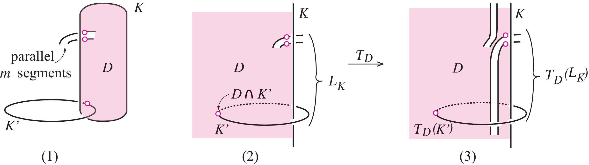
as follows. We cut $\mathcal{E}(K)$ along $D$ . We have resulting two sides obtained from $D$ . Then we reglue the two sides by rotating either of the sides $360$ degrees so that the mapping class of the restriction $T|_{\partial\mathcal{E}(K)}:\partial\mathcal{E}(K)\rightarrow\partial\mathcal{E}(K)$ defines the left-handed Dehn twist about $\partial D$ , see Figure 8(1). Such an operation defines the former homeomorphism $T_{D}:\mathcal{E}(K)\rightarrow\mathcal{E}(K)$ . If $m$ segments of $L_{K}$ pass through $D$ , then $T(L_{K})$ is obtained from $L_{K}$ by adding a full twist braid $\Delta_{m}^{2}$ near $D$ . In the case $m=2$ , see Figure 8(2). Notice that $T_{D}:\mathcal{E}(K)\rightarrow\mathcal{E}(K)$ determines the latter homeomorphism

H=H_{D}:\mathcal{E}(L)(=\mathcal{E}(K\cup L_{K}))\rightarrow\mathcal{E}(K\cup T(L_{K})).

For any integer $\ell\neq 0$ , we have a homeomorphism of the $\ell$ th power $T^{\ell}=T_{D}^{\ell}:\mathcal{E}(K)\rightarrow\mathcal{E}(K)$ so that $T^{\ell}|_{\partial\mathcal{E}(K)}:\partial\mathcal{E}(K)\rightarrow\partial\mathcal{E}(K)$ is the $\ell$ th power of the left-handed Dehn twist about $\partial D$ . Observe that $T^{\ell}=T_{D}^{\ell}$ converts $L=K\cup L_{K}$ into a link $K\cup T^{\ell}(L_{K})$ in $S^{3}$ such that $S^{3}\setminus L$ is homeomorphic to $S^{3}\setminus(K\cup T^{\ell}(L_{K}))$ . We denote by $H_{D}^{\ell}$ , a homeomorphism: $\mathcal{E}(L)(=\mathcal{E}(K\cup L_{K}))\rightarrow\mathcal{E}(K\cup T^{\ell}(L_{K}))$ .

The following remark is used in the proof of Proposition 1.3.

Remark 2.13.

Let $L$ be a link in $S^{3}$ . Suppose that $L$ contains two unknotted components $K$ and $K^{\prime}$ such that $K\cup K^{\prime}$ is the Hopf link. Let $D$ be a disk bounded by the longitude of $\mathcal{N}(K)$ . We assume that parallel $m\geq 1$ segments of $L_{K}\setminus K^{\prime}$ pass through $D$ , see Figure 9(1) in the case $m=2$ . ( $L_{K}\setminus K^{\prime}$ may intersect with the disk bounded by the longitude of $\mathcal{N}(K^{\prime})$ .) Pushing $D$ along the meridian of $\mathcal{N}(K)$ , one can put the resulting disk $D$ as in Figure 9(2). The small circles in Figure 9(2) indicate the intersection between $L_{K}$ and $D$ . Now we consider the disk twist $T$ about $D$ , that is, we cut $\mathcal{E}(K)$ along $D$ and we reglue the two sides obtained from $D$ by rotating one of the sides by 360 degrees. In this case, one can choose the intersection point $D\cap K^{\prime}$ as an origin of the rotation of $D$ . As a result, we get a local diagram of the link $T(L_{K})$ shown in Figure 9(3) so that $T=T_{D}$ fixes $K^{\prime}$ . (See $K^{\prime}$ and $T_{D}(K^{\prime})$ in Figure 9(2)(3).)

3. Proof of Proposition 1.3

We introduce a sequence of braids $w_{2n}\in SW_{2n}$ . Let

w_{6}=\sigma_{2}^{-1}\sigma_{1}^{-1}\sigma_{3}\sigma_{2}\sigma_{4}\sigma_{3}^{2}\sigma_{4}\sigma_{3}=\sigma_{2}^{-1}\sigma_{1}^{-1}\sigma_{3}\sigma_{2}\sigma_{4}\sigma_{3}\sigma_{4}\sigma_{3}\sigma_{4}\in SB_{(5)},

see Figure 10(1). (For the definition of the subgroup $SB_{(m-1)}$ of $SB_{m}$ , see Section 2.3.) Since ${}^{w_{6}}{\bf A}$ is isotopic to ${\bf A}$ relative to $\partial{\bf A}$ , we have $w_{6}\in SW_{6}$ . In order to define a sequence of braids $w_{8},w_{10},\cdots$ , we introduce $x_{4n+8},y_{4n+8}\in SB_{(4n+7)}$ for each $n\geq 0$ as follows.

	$\displaystyle x_{4n+8}$	$\displaystyle=$	$\displaystyle\sigma_{5}\sigma_{2}^{-1}\sigma_{1}^{-1}(\sigma_{3}\sigma_{4}\cdots\sigma_{4n+5})(\sigma_{2}\sigma_{3}\cdots\sigma_{4n+4})\sigma_{4n+6}(\sigma_{4n+5})^{2}\sigma_{4n+6},$
	$\displaystyle y_{4n+8}$	$\displaystyle=$	$\displaystyle(\sigma_{1}\sigma_{2}\cdots\sigma_{4n+5})^{4}\sigma_{4n+6}\sigma_{4n+5}\sigma_{4n+4}(\sigma_{4n+3})^{2}\sigma_{4n+4}\sigma_{4n+5}\sigma_{4n+6},$

see Figure 11(1)(2). It is straightforward to check that ${}^{b}{\bf A}$ is isotopic to ${\bf A}$ relative to $\partial{\bf A}$ when $b=x_{4n+8}$ , $y_{4n+8}$ . Thus $x_{4n+8}$ , $y_{4n+8}\in SW_{4n+8}$ . We let

w_{4n+8}=x_{4n+8}(y_{4n+8})^{n}\in SB_{(4n+7)}\cap SW_{4n+8},

where $(y_{8})^{0}=1\in SB_{(7)}$ . For example, in the case of $n=0$ ,

w_{8}=x_{8}(y_{8})^{0}=\sigma_{5}\sigma_{2}^{-1}\sigma_{1}^{-1}\sigma_{3}\sigma_{4}\sigma_{5}\sigma_{2}\sigma_{3}\sigma_{4}\sigma_{6}\sigma_{5}^{2}\sigma_{6},

see Figure 10(2). Notice that the last two strings ( $(4n+7)$ th and $(4n+8)$ th strings) of both $x_{4n+8}$ and $y_{4n+8}$ define the identity $1\in SB_{2}$ , see Figure 11(1)(2). Thus we obtain the $(4n+6)$ -spherical braid by removing the last two strings from $w_{4n+8}$ . In the case $n\geq 1$ , we denote by $w_{4n+6}$ , the resulting $(4n+6)$ -braid. Said differently if we let $x_{4n+6}$ (resp. $y_{4n+6}$ ) be the $(4n+6)$ -spherical braid obtained from $x_{4n+8}$ (resp. $y_{4n+8}$ ) by removing the last two strings from $x_{4n+8}$ (resp. $y_{4n+8}$ ), then $w_{4n+6}$ is given by

w_{4n+6}=x_{4n+6}(y_{4n+6})^{n},

see Figure 11(3)(4). Clearly $w_{4n+6}\in SW_{4n+6}$ , since $w_{4n+8}\in SW_{4n+8}$ .

Remark 3.1.

The braid $w_{6}\in SW_{6}$ is not the same as the braid which is obtained from $w_{8}$ as above. The latter braid is not used in the rest of the paper.

In the proof of the next lemma, we use some basic facts on train tracks of pseudo-Anosov homeomorphisms. See [4, 26] for more details. For a quick review about train tracks, see [21, Section 2.1] which contains terms and basic facts needed in this paper.

Lemma 3.2.

The braid $\underline{w_{6}}\in B_{5}$ is pseudo-Anosov, and $\lambda(\underline{w_{6}})$ equals $\kappa$ , where $\kappa$ is the constant given in Proposition 1.3.

Proof.

We choose a train track $\tau\subset D_{5}$ with non-loop edges $p_{1},\cdots,p_{6}$ as in Figure 12(1), where $c_{1},\cdots,c_{5}$ are punctures of $D_{5}$ . Each component of $D_{5}\setminus\tau$ is either a $1$ -gon with one puncture, a $3$ -gon (without punctures), or a $1$ -gon containing the boundary of the disk (see the illustration of $\tau\subset D_{5}\times\{0\}$ on the bottom of Figure 12(3)). We consider the braid $\underline{w_{6}}$ with base points $c_{1},\cdots,c_{5}$ . We push $\tau$ on $D_{5}$ along the suspension flow on $S^{3}\setminus\mathrm{br}(\underline{w_{6}})$ , then we get the train track $\tau^{\prime}$ on $D_{5}\times\{1\}$ illustrated in Figure 12(2). This implies that there exists a representative $f\in\Gamma(\underline{w_{6}})$ such that $\tau^{\prime}=f(\tau)$ . Here, the edge $(p_{i})$ of $\tau^{\prime}$ in Figure 12(2) denotes the image of $p_{i}$ under $f$ .

We see that $f(\tau)$ is carried by $\tau$ , and hence $\tau$ is an invariant train track¹¹ 1 One can use the software Trains [14] to find invariant train tracks for pseudo-Anosov braids. for $\Gamma(\underline{w_{6}})$ . Let $N(\tau)$ be a fibered (tie) neighborhood of $\tau$ whose fibers (ties) are segment given by a retraction $\mathfrak{R}:\mathcal{N}(\tau)\to\tau$ . Then we get a train track representative $\mathfrak{p}=\mathfrak{R}\circ f|_{\tau}:\tau\rightarrow\tau$ for $\Gamma(\underline{w_{6}})$ . It turns out that $p_{1},\cdots,p_{6}$ are ²² 2 We recall the terminology in Bestvina-Handel [4]. An edge $e$ of $\tau$ for a train track representative $\mathfrak{p}:\tau\rightarrow\tau$ is called infinitesimal if $e$ is eventually periodic under $\mathfrak{p}$ . Otherwise $e$ is called real.real edges for $\mathfrak{p}$ , and other loop edges of $\tau$ are periodic under $\mathfrak{p}$ , and hence they are infinitesimal edges. The incident matrix $M_{\mathfrak{p}}$ with respect to real edges is given by

M_{\mathfrak{p}}=\left[\begin{array}[]{cccccc}2&0&0&0&0&1\\ 2&0&0&2&1&0\\ 1&0&1&1&1&0\\ 0&0&2&1&2&0\\ 1&0&0&0&0&0\\ 0&1&0&0&0&0\end{array}\right].

For example, we get $\ {}^{t}\!\left[\begin{array}[]{cccccc}0&0&1&2&0&0\end{array}\right]$ for the $3$ rd column of $M_{\mathfrak{p}}$ , since $f(p_{3})$ passes through $p_{3}$ once and $p_{4}$ twice in either direction. (See the edge path $(p_{3})$ in Figure 12(2).) Since the $5$ th power $M_{\mathfrak{p}}^{5}$ is positive, $M_{\mathfrak{p}}$ is Perron-Frobenius and we conclude that $\underline{w_{6}}$ is pseudo-Anosov. The characteristic polynomial of $M_{\mathfrak{p}}$ equals

(t-1)^{2}(t^{4}-2t^{3}-2t^{2}-2t+1),

and the largest root $\kappa$ of the second factor gives us $\lambda(\underline{w_{6}})$ . ∎

The type of singularities of the (un)stable foliation for the pseudo-Anosov homeomorphism $\Phi=\Phi_{w_{6}}:\varSigma_{0,6}\rightarrow\varSigma_{0,6}$ can be read from the topological types of components of $\varSigma_{0,6}\setminus\tau$ . See [4, Section 3.4] which describes a construction of invariant measured foliations. Notice that two component of $\varSigma_{0,6}\setminus\tau$ are non punctured $3$ -gons. The other components are once punctured $1$ -gons. Thus exactly two points in the interior of $\varSigma_{0,6}$ have $3$ prongs and each puncture of $\varSigma_{0,6}$ has a $1$ prong.

Observe that $\mathrm{br}(\underline{w_{6}})$ is the link with $3$ components. The following lemma says that complements of both links $\mathrm{br}(\underline{w_{6}})$ and $L_{0}$ (Figure 1) are the same.

Lemma 3.3.

${\mathbb{T}}_{\underline{w_{6}}}$ is homeomorphic to $S^{3}\setminus L_{0}$ . In particular $S^{3}\setminus L_{0}$ is a hyperbolic fibered $3$ -manifold.

Proof.

We use another diagram of $L_{0}$ illustrated in Figure 13(1). The link $L_{0}$ contains two unknots $K$ and $K^{0}$ so that $K\cup K^{0}$ is the Hopf link. We take the disk $D$ bounded by the longitude of $\mathcal{N}(K)$ . We may assume that $L_{0}\setminus K(=(L_{0})_{K})$ intersect with $D$ at the three points indicated by small circles in the same figure. We apply the argument (in the case $m=2$ ) of Remark 2.13, and consider the disk twist about $D$ , see Figure 13(2). It turns out that $K\cup T_{D}(L_{0}\setminus K)$ is of the form $\mathrm{br}(\underline{w_{6}})$ , see Figure 13(3). Thus $S^{3}\setminus L_{0}$ is homeomorphic to $S^{3}\setminus\mathrm{br}(\underline{w_{6}})(=S^{3}\setminus(K\cup T_{D}(L_{0}\setminus K)))$ . Since ${\mathbb{T}}_{\underline{w_{6}}}$ is homeomorphic to $S^{3}\setminus\mathrm{br}(\underline{w_{6}})$ and $\underline{w_{6}}$ is pseudo-Anosov by Lemma 3.2, we complete the proof. ∎

Let $F_{g,n}$ be a compact, connected, orientable surface of genus $g$ with $n$ boundary components. Let $M_{0}$ be the exterior of the link $L_{0}$ . By Lemma 3.3, we let $a_{6}\in H_{2}(M_{0},\partial M_{0};{\mathbb{Z}})$ be the homology class of the $F_{0,6}$ -fiber of the fibration on $M_{0}$ whose monodromy is described by $w_{6}\in SB_{6}$ .

Lemma 3.4.

${\mathbb{T}}_{\underline{w_{4n+8}}}$ is homeomorphic to ${\mathbb{T}}_{\underline{w_{6}}}$ for each $n\geq 0$ . In particular $\underline{w_{4n+8}}\in B_{4n+7}$ is pseudo-Anosov for each $n\geq 0$ .

Proof.

We prove that $S^{3}\setminus\mathrm{br}(\underline{w_{4n+8}})$ is homeomorphic to $S^{3}\setminus\mathrm{br}(\underline{w_{6}})$ . To do this, we use Remark 2.13 twice. The braided link $\mathrm{br}(\underline{w_{6}})$ contains two unknotted components, the braid axis $K^{\prime}$ and the closure of the last string of $\underline{w_{6}}$ , say $K$ so that $K\cup K^{\prime}$ is the Hopf link. Let $D^{\prime}$ be the disk bounded by the longitude of $\mathcal{N}(K^{\prime})$ . Consider the $n$ th power of the disk twist $T_{D^{\prime}}^{n}$ for $n\geq 0$ . Following Remark 2.13, we take the point $D^{\prime}\cap K$ as an origin of the rotation of $D^{\prime}$ for the disk twists $T_{D^{\prime}}^{n}$ . Then we have the diagram of $K^{\prime}\cup T_{D^{\prime}}^{n}(\mathrm{br}(\underline{w_{6}})\setminus K^{\prime})=K^{\prime}\cup T_{D^{\prime}}^{n}(\mathrm{cl}(\underline{w_{6}}))$ shown in Figure 14(2). Note that $T_{D^{\prime}}^{n}(\mathrm{cl}(\underline{w_{6}}))$ is isotopic to $\mathrm{cl}(\underline{w_{6}}\Delta^{2n})$ , that is the closure of $\underline{w_{6}}\Delta^{2n}=\underline{w_{6}}(\sigma_{1}\sigma_{2}\sigma_{3}\sigma_{4})^{5n}$ . Thus

K^{\prime}\cup T_{D^{\prime}}^{n}(\mathrm{br}(\underline{w_{6}})\setminus K^{\prime})=\mathrm{br}(\underline{w_{6}}\Delta^{2n}),

and $H_{D^{\prime}}^{n}$ is a homeomorphism from $\mathcal{E}(\mathrm{br}(\underline{w_{6}}))$ to $\mathcal{E}(K^{\prime}\cup T_{D^{\prime}}^{n}(\mathrm{br}(\underline{w_{6}})\setminus K^{\prime}))\simeq\mathcal{E}(\mathrm{br}(\underline{w_{6}}\Delta^{2n}))$ . (See Section 2.7 for $H_{D^{\prime}}^{n}$ .) The closure of the last string of $\underline{w_{6}}\Delta^{2n}\in B_{5}$ is an unknot, say $K^{\prime\prime}$ which bounds a disk $D^{\prime\prime}$ . (In the case $n=0$ , we have $K=K^{\prime\prime}$ , $D=D^{\prime\prime}$ and $H_{D^{\prime}}^{n}$ equals the identity map.) We apply the argument of Remark 2.13, and consider the disk twist $T_{D^{\prime\prime}}$ taking the point of $D^{\prime\prime}\cap K^{\prime}$ as an origin of the rotation of the disk $D^{\prime\prime}$ for $T_{D^{\prime\prime}}$ . It turns out that

K^{\prime\prime}\cup T_{D^{\prime\prime}}(\mathrm{br}(\underline{w_{6}}\Delta^{2n})\setminus K^{\prime\prime})=\mathrm{br}(\underline{x_{4n+8}}\ \underline{(y_{4n+8})^{n}})(=\mathrm{br}(\underline{w_{4n+8}})).

To see the equality, we first note that $\mathrm{br}(\underline{w_{6}}\Delta^{2n})\setminus(K^{\prime}\cup K^{\prime\prime})$ intersects with $D^{\prime\prime}$ at $2+4n$ points, see Figure 14(2). We arrange, by an isotopy, $2+4n$ intersection points in a line which is parallel to $K^{\prime\prime}$ . Then view the image $T_{D^{\prime\prime}}(\mathrm{br}(\underline{w_{6}}\Delta^{2n})\setminus K^{\prime\prime})$ following the local move under the disk twist $T_{D^{\prime\prime}}$ , see Figure 9(2)(3). (Here $m$ in Figure 9(1) is equal to $2+4n$ .) Figure 15 explains this procedure in the case $n=2$ .

The above equality implies that $H_{D^{\prime\prime}}$ is a homeomorphism from $\mathcal{E}(\mathrm{br}(\underline{w_{6}}\Delta^{2n}))$ to $\mathcal{E}(K^{\prime\prime}\cup T_{D^{\prime\prime}}(\mathrm{br}(\underline{w_{6}}\Delta^{2n})\setminus K^{\prime\prime}))\simeq\mathcal{E}(\mathrm{br}(\underline{w_{4n+8}}))$ . The composition of the maps $H_{D^{\prime\prime}}\circ H_{D^{\prime}}^{n}$ sends $\mathcal{E}(\mathrm{br}(\underline{w_{6}}))$ to $\mathcal{E}(\mathrm{br}(\underline{w_{4n+8}}))$ . Thus $S^{3}\setminus\mathrm{br}(\underline{w_{6}})$ is homeomorphic to $S^{3}\setminus\mathrm{br}(\underline{w_{4n+8}})$ . Since ${\mathbb{T}}_{\underline{w_{6}}}=S^{3}\setminus\mathrm{br}(\underline{w_{6}})$ is hyperbolic, we conclude that by Lemma 2.5, the braid $\underline{w_{4n+8}}$ is pseudo-Anosov. ∎

By Lemma 3.4, we let $a_{4n+8}\in H_{2}(M_{0},\partial M_{0};{\mathbb{Z}})$ be the homology class of the $F_{0,4n+8}$ -fiber of the fibration on $M_{0}$ whose monodromy is described by $w_{4n+8}$ . To study properties of such a fibered class, we take a $3$ -punctured disk $F\simeq\varSigma_{0,4}$ embedded in $S^{3}\setminus\mathrm{br}(\underline{w_{6}})$ so that $F$ is bounded by the unknotted component $K\subset\mathrm{br}(\underline{w_{6}})$ , i.e, $F$ is an interior of the disk $D$ removed the set of $3$ points $(\mathrm{br}(\underline{w_{6}})\setminus K)\cap D$ . To choose an orientation of $F$ , we consider an orientation of the last string of $\underline{w_{6}}$ from the top to the bottom. This determines an orientation of $K$ (see Figure 14(1)), and we have an orientation of $F$ induced by $K$ . Let $\bar{F}$ be the oriented disk with $3$ holes (i.e, sphere with $4$ boundary components) embedded in $\mathcal{E}(\mathrm{br}(\underline{w_{6}}))$ , which is obtained from $D$ removed the interiors of the $3$ disks whose centers are the above $3$ points. The fibered class $a_{4n+8}$ can be expressed by using $a_{6}$ and $[\bar{F}]\in H_{2}(M_{0},\partial M_{0};{\mathbb{Z}})$ as follows.

Lemma 3.5.

We have $a_{4n+8}=(n+1)a_{6}+[\bar{F}]\in H_{2}(M_{0},\partial M_{0};{\mathbb{Z}})$ for each $n\geq 0$ . In particular, the ray of $a_{4n+8}$ through the origin goes to the ray of $a_{6}$ as $n$ goes to $\infty$ .

Proof.

Recall that $F_{a_{6}}$ is a minimal representative of $a_{6}$ . In other words, $F_{a_{6}}$ is a $F_{0,6}$ -fiber of the fibration on $M_{0}$ associated to $a_{6}$ . We consider the oriented sum $nF_{a_{6}}+\bar{F}$ which is an oriented surface embedded in $M_{0}$ . This surface is obtained by the cut and paste construction of parallel $n$ copies of $F_{a_{6}}$ and a copy of $\bar{F}$ . (For the construction of the oriented sum, see [31, p104] or [7, Section 5.1.1].) We take a surface $F^{\prime\prime}$ embedded in $M_{0}$ , which is a disk with $(3+4n)$ holes as follows. Consider the disk $D^{\prime\prime}$ bounded by the longitude of $\mathcal{N}(K^{\prime\prime})$ . Then remove the interiors of small $(3+4n)$ disks from $D^{\prime\prime}$ whose centers are the $(3+4n)$ intersection points $(\mathrm{br}(\underline{w_{6}}\Delta^{2n})\setminus K^{\prime\prime})\cap D^{\prime\prime}$ , see Figure 14(2). We denote by $F^{\prime\prime}$ , the resulting disk with $(3+4n)$ holes. We see that the homeomorphism $H_{D^{\prime}}^{n}:\mathcal{E}(\mathrm{br}(\underline{w_{6}}))\rightarrow\mathcal{E}(\mathrm{br}(\underline{w_{6}}\Delta^{2n}))$ in the proof of Lemma 3.4 sends $nF_{a_{6}}+\bar{F}$ to $F^{\prime\prime}$ . Hence

[F^{\prime\prime}]=[nF_{a_{6}}+\bar{F}]=na_{6}+[\bar{F}]\in H_{2}(M_{0},\partial M_{0};{\mathbb{Z}}).

Obviously $[H_{D^{\prime}}^{n}(F_{a_{6}})]=[F_{a_{6}}](=a_{6})$ . We now consider the oriented sum $H_{D^{\prime}}^{n}(F_{a_{6}})+F^{\prime\prime}$ . Then $H_{D^{\prime\prime}}:\mathcal{E}(\mathrm{br}(\underline{w_{6}}\Delta^{2n}))\rightarrow\mathcal{E}(\mathrm{br}(\underline{w_{4n+8}}))$ in the proof of Lemma 3.4 sends $H_{D^{\prime}}^{n}(F_{a_{6}})+F^{\prime\prime}$ to the $F_{0,4n+8}$ -fiber of the fibration on $M_{0}$ associated to $a_{4n+8}$ . Putting all things together, we have

a_{4n+8}=[H_{D^{\prime}}^{n}(F_{a_{6}})+F^{\prime\prime}]=[H_{D^{\prime}}^{n}(F_{a_{6}})]+[F^{\prime\prime}]=a_{6}+na_{6}+[\bar{F}]=(n+1)a_{6}+[\bar{F}].

Thus

\displaystyle\lim_{n\to\infty}\tfrac{a_{4n+8}}{n+1}=\displaystyle\lim_{n\to\infty}(a_{6}+\tfrac{[\bar{F}]}{n+1})=a_{6}.

This completes the proof. ∎

Since the normalized entropy function $\mathrm{Ent}$ is constant on each ray through the origin in the fibered cone, Lemmas 3.2, 3.3, 3.4 and 3.5 tell us that

(3.1)

\lim_{n\to\infty}|\chi(F_{0,4n+8})|\log(\lambda(w_{4n+8}))=|\chi(F_{0,6})|\log(\lambda(w_{6}))=4\log\kappa.

Since $|\chi(F_{0,4n+8})|=4n+6$ goes to $\infty$ as $n$ does, and the right-hand side is constant, we conclude that

(3.2)

\displaystyle\lim_{n\to\infty}\log\lambda(w_{4n+8})=0.

Let $\Omega$ be a fibered face of $M_{0}$ such that $a_{6}\in int(C_{\Omega})$ . Lemma 3.5 implies that $a_{4n+8}\in int(C_{\Omega})$ for $n$ large. We shall prove in Lemma 3.6 that the fibered class $a_{4n+8}$ lies in $int(C_{\Omega})$ for each $n\geq 0$ . Recall that $K$ and $K^{\prime}$ are the unknotted components of $\mathrm{br}(\underline{w_{6}})$ . We choose an orientation of $K^{\prime}$ as in Figure 14(1). For an embedded surface $\hat{S}$ in $M_{0}=\mathcal{E}(\mathrm{br}(\underline{w_{6}}))$ , we denote by $\partial_{K}(\hat{S})$ and $\partial_{K^{\prime}}(\hat{S})$ , the components of the boundary $\partial\hat{S}$ of $\hat{S}$ which lie on $\partial\mathcal{N}(K)$ and $\partial\mathcal{N}(K^{\prime})$ respectively. Let $\hat{\Phi}:F_{0,6}\rightarrow F_{0,6}$ be a pseudo-Anosov homeomorphism whose mapping class $[\hat{\Phi}]$ is described by $w_{6}$ . (Thus ${\mathbb{T}}_{[\hat{\Phi}]}$ is homeomorpphic to $\mathcal{E}(\mathrm{br}(\underline{w_{6}}))\simeq M_{0}$ .)

Lemma 3.6.

We have $a_{4n+8}\in int(C_{\Omega})$ for each $n\geq 0$ .

Proof.

The minimal representative $F_{a_{6}}$ is transverse to the suspension flow $\hat{\Phi}^{t}$ obviously, but $\bar{F}$ is not, since both $\partial_{K}\bar{F}$ and $\partial_{K^{\prime}}\bar{F}$ are parallel to flow lines of $\hat{\Phi}^{t}$ . (See also Figure 16(3) and its caption.) We prove that the oriented sum $(n+1)F_{a_{6}}+\bar{F}$ for $n\geq 0$ is transverse to $\hat{\Phi}^{t}$ (up to isotopy) and it intersects every flow line. This means that $(n+1)F_{a_{6}}+\bar{F}$ is a cross-section to $\hat{\Phi}^{t}$ for $\mathcal{E}(\mathrm{br}(\underline{w_{6}}))$ . By Theorem 2.2(3), we have $a_{4n+8}=[(n+1)F_{a_{6}}+\bar{F}]\in int(C_{\Omega})$ .

By the proof of Lemma 3.5, $(n+1)F_{a_{6}}+\bar{F}$ becomes a fiber of the fibration on $M_{0}$ associated to $a_{4n+8}$ . Hence we may assume that

(3.3)

F_{a_{4n+8}}=(n+1)F_{a_{6}}+\bar{F}.

We have the meridian and longitude basis $\{m_{K},\ell_{K}\}$ for $\partial\mathcal{N}(K)$ and $\{m_{K^{\prime}},\ell_{K^{\prime}}\}$ for $\partial\mathcal{N}(K^{\prime})$ . It follows that

	$\displaystyle{[}\partial_{K}F_{a_{4n+8}}{]}$	$\displaystyle=$	$\displaystyle(n+1)m_{K}+\ell_{K}\neq\pm\ell_{K}\in H_{1}(\partial\mathcal{N}(K))\ \mbox{and}$
	$\displaystyle{[}\partial_{K^{\prime}}F_{a_{4n+8}}{]}$	$\displaystyle=$	$\displaystyle(n+1)\ell_{K^{\prime}}+m_{K^{\prime}}\neq\pm m_{K^{\prime}}\in H_{1}(\partial\mathcal{N}(K^{\prime})).$

This implies that both $\partial_{K}F_{a_{4n+8}}$ and $\partial_{K^{\prime}}F_{a_{4n+8}}$ are transverse to every flow line of $\hat{\Phi}^{t}$ , since $[\partial_{K}\bar{F}]=\ell_{K}$ and $[\partial_{K}^{\prime}\bar{F}]=m_{K^{\prime}}$ . By (3.3), $F_{a_{4n+8}}$ is an oriented sum obtained from the $(n+1)$ copies of $F_{a_{6}}$ and the surface $\bar{F}$ . Hence the shape of the embedded surface $F_{a_{4n+8}}$ in $M_{0}$ is of a ‘spiral staircase’ which turns round $(n+1)$ times along $\ell_{K}$ . Therefore $F_{a_{4n+8}}$ is transverse to $\hat{\Phi}^{t}$ . Moreover $F_{a_{4n+8}}$ intersects every flow line of $\hat{\Phi}^{t}$ (by construction of $(n+1)F_{a_{6}}+\bar{F}(=F_{a_{4n+8}})$ ), since so does $F_{a_{6}}$ . This completes the proof. ∎

Lemma 3.7.

If $n\geq 1$ , then $w_{4n+6}$ is pseudo-Anosov and the equality $\lambda(w_{4n+6})=\lambda(w_{4n+8})$ holds. In particular ${\mathbb{T}}_{w_{4n+6}}$ is a hyperbolic fibered $3$ -manifold obtained from ${\mathbb{T}}_{w_{4n+8}}$ by Dehn fillings about the two cusps along the boundary slopes of the fiber associated to $a_{w_{4n+8}}$ .

We work on the cusped $3$ -manifold ${\mathbb{T}}_{w_{6}}={\mathbb{T}}_{\underline{w_{6}}}\simeq S^{3}\setminus L_{0}$ instead of $M_{0}$ with boundary. To prove Lemma 3.7, we shall construct an invariant train track for $\Gamma(w_{4n+8})$ concretely, and study types of singularities of the unstable foliation $\mathcal{F}_{w_{4n+8}}$ of the pseudo-Anosov homeomorphism $\Phi_{w_{4n+8}}:\varSigma_{0,4n+8}\rightarrow\varSigma_{0,4n+8}$ which represents $\Gamma(w_{4n+8})$ . The same idea in [21, Section 3] for the construction of train tracks can be used. We repeat a similar argument modifying some claims of [21] in a suitable way for the present paper. Hereafter we use basic properties on branched surfaces. See [25] for more details on the theory of branched surfaces.

By using the pseudo-Anosov homeomorphism $\Phi=\Phi_{w_{6}}:\varSigma_{0,6}\rightarrow\varSigma_{0,6}$ , we build the mapping torus

{\mathbb{T}}_{w_{6}}=\varSigma_{0,6}\times{\mathbb{R}}/_{(x,t+1)=(\Phi(x),t)}

for $x\in\varSigma_{0,6}$ and $t\in{\mathbb{R}}$ . Given a subset $U\subset\varSigma_{0,6}$ , we define $U^{t}\subset{\mathbb{T}}_{w_{6}}$ to be the image $U\times\{t\}$ under the projection $p:\varSigma\times{\mathbb{R}}\rightarrow{\mathbb{T}}_{w_{6}}$ . We have an orientation preserving homeomorphism

h:S^{3}\setminus\mathrm{br}(\underline{w_{6}})\to{\mathbb{T}}_{w_{6}}.

Recall that $F$ is an oriented $4$ -punctured sphere in $S^{3}\setminus\mathrm{br}(\underline{w_{6}})$ . Choose an orientation of $\varSigma_{0,6}^{v}=\varSigma_{0,6}\times\{v\}$ for each $v\in{\mathbb{R}}$ so that its normal direction coincides with the flow $\Phi^{t}$ direction. We shall capture the image $h(F)$ in ${\mathbb{T}}_{w_{6}}$ . To do this, let $s$ be a segment between the punctures $c_{5}$ and $c_{6}$ . Since $\Phi$ fixes $c_{5}$ and $c_{6}$ pointwise (see the last two strings of $w_{6}$ in Figure 10(1)), $s\cup\Phi(s)$ bounds a $2$ -gon. Viewing the image $\Phi(s)$ , we see that the $2$ -gon contains the punctures $c_{1}$ and $c_{2}$ , see Figure 16. Such a $2$ -gon removed $c_{1}$ and $c_{2}$ is denoted by $S\subset\varSigma_{0,6}$ . The segment $s^{0}=s\times\{0\}$ is connected to $s^{1}=s\times\{1\}$ , and these segments make a flowband $J=[s^{0},s^{1}]$ which is illustrated in Figure 16(3). Since $s^{1}=(\Phi(s))^{0}$ in ${\mathbb{T}}_{w_{6}}$ , the union

S^{0}\cup J(=(S\times\{0\})\cup J)\subset{\mathbb{T}}_{w_{6}}

defines a $4$ -punctured sphere, see Figure 16(3). The set of punctures of $F$ maps to the set of punctures of $S^{0}\cup J$ under $h$ . This tells us that $h(F)=S^{0}\cup J$ up to isotopy. For simplicity, $S^{0}\cup J$ in ${\mathbb{T}}_{w_{6}}$ is denoted by $F$ .

We choose $0<\epsilon<2\epsilon<1$ . We push $F(=S^{0}\cup J)\subset{\mathbb{T}}_{w_{6}}$ along the flow lines for $\epsilon$ times so that the resulting $4$ -punctured sphere, denoted by $F^{\epsilon}$ , satisfies

F^{\epsilon}\cap\varSigma_{0,6}^{\epsilon}=S^{\epsilon}(=S\times\{\epsilon\}),

see Figure 18(2) for $S^{\epsilon}$ . By using $F^{\epsilon}$ and $\varSigma_{0,6}^{2\epsilon}=\varSigma_{0,6}\times\{2\epsilon\}$ which corresponds to a fiber $F_{a_{6}}$ of the fibration on $M_{0}$ , we set

\widehat{\mathcal{B}}=F^{\epsilon}\cup\varSigma_{0,6}^{2\epsilon}.

We get the branched surface $\mathcal{B}$ from $\widehat{\mathcal{B}}$ (which agrees with the orientations of $F^{\epsilon}$ and $\varSigma_{0,6}^{2\epsilon}$ ) after we modify the flowband

[s^{\epsilon},(\Phi(s))^{\epsilon}]=[s^{\epsilon},s^{1}]\cup[(\Phi(s))^{0},(\Phi(s))^{\epsilon}]

of $F^{\epsilon}$ near the segment $s^{2\epsilon}=F^{\epsilon}\cap\varSigma_{0,6}^{2\epsilon}\in[s^{\epsilon},s^{1}]$ . (cf. For the illustration of this modification, see [21, Figure 14].) By Lemmas 3.4 and 3.5, there exists a $\varSigma_{0,4n+8}$ -fiber of the fibration on ${\mathbb{T}}_{w_{6}}$ with the monodromy $\Gamma(w_{4n+8})$ . We denote such a fiber by $\varSigma_{w_{4n+8}}$ . By (3.3), we have

(3.4)

\varSigma_{w_{4n+8}}=F+(n+1)\varSigma_{0,6}.

By the construction of $\mathcal{B}$ , we see that $\varSigma_{w_{4n+8}}$ is carried by $\mathcal{B}$ .

Let $\widehat{\mathcal{F}}\subset{\mathbb{T}}_{w_{6}}$ be the suspension of the unstable foliation $\mathcal{F}$ for $\Phi$ . We may assume that the train track $\tau\subset D_{5}$ in the proof of Lemma 3.2 lies on $\varSigma_{0,6}$ . Then $\tau$ is an invariant train track for $\Gamma(w_{6})=[\Phi]$ . Theorem 2.2(1)(2) and Lemma 3.6 imply the following.

Lemma 3.8.

The pseudo-Anosov homeomorphism $\Phi_{w_{4n+8}}:\varSigma_{w_{4n+8}}\rightarrow\varSigma_{w_{4n+8}}$ is precisely the first return map $:\varSigma_{w_{4n+8}}\rightarrow\varSigma_{w_{4n+8}}$ of $\Phi^{t}$ . Moreover $\mathcal{F}_{w_{4n+8}}=\widehat{\mathcal{F}}\cap\varSigma_{w_{4n+8}}$ .

We turn to the construction of the branched surface $\mathcal{B}_{\Omega}$ which carries $\widehat{\mathcal{F}}$ . First of all, we note that $\tau$ is obtained from $\Phi(\tau)$ by folding edges (or zipping edges), see Figure 17. We choose a family of train tracks $\{\tau_{t}\}_{0\leq t\leq 1}$ on $\varSigma_{0,6}$ as follows.

(1)

$\tau_{0}=\Phi(\tau)$ .
(2)

$\tau_{t}$ at $t=\epsilon$ is a train track illustrated in Figure 17(middle in the left column).
(3)

$\tau_{t}=\tau$ for $2\epsilon\leq t\leq 1$ .
(4)

If $0\leq s<t\leq 2\epsilon$ , then $\tau_{t}=\tau_{s}$ or $\tau_{t}$ is obtained from $\tau_{s}$ by folding edges between a cusp of $\tau_{s}$ .

We let

\mathcal{B}_{\Omega}=\bigcup_{0\leq t\leq 1}\tau_{t}\times\{t\}\subset{\mathbb{T}}_{w_{6}}.

Since $\tau_{1}\times\{1\}=\tau_{0}\times\{0\}$ in ${\mathbb{T}}_{w_{6}}$ (see the above conditions (1)(3)), it follows that $\mathcal{B}_{\Omega}$ is a branched surface. Since the invariant train track $\tau$ carries the unstable foliation $\mathcal{F}$ , we see that $\mathcal{B}_{\Omega}$ carries $\widehat{\mathcal{F}}$ . It is not hard to see that $\mathcal{B}_{\Omega}$ is transverse to the previous branched surface $\mathcal{B}$ (up to isotopy). Let

(3.5)

\tau_{4n+8}=\varSigma_{w_{4n+8}}\cap\mathcal{B}_{\Omega},

which is a branched $1$ -manifold, see Figure 19(1). Since $\varSigma_{w_{4n+8}}$ is carried by $\mathcal{B}$ , we may put $(n+1)$ copies of $\varSigma_{0,6}$ which is a part of $\varSigma_{w_{4n+8}}$ (see (3.4)) into $\varSigma_{0,6}\times(2\epsilon,1)$ . We may also assume that a copy of $F$ which is another part of $\varSigma_{w_{4n+8}}$ satisfies that $S^{\epsilon}=F\cap\varSigma_{0,6}^{\epsilon}$ . Then intersections $\varSigma_{0,6}^{2\epsilon}\cap\mathcal{B}_{\Omega}$ and $S^{\epsilon}\cap\mathcal{B}_{\Omega}$ (see Figure 18) together with $s^{2\epsilon}=F^{\epsilon}\cap\varSigma_{0,6}^{2\epsilon}$ determine $\tau_{4n+8}$ . More concretely, $\tau_{4n+8}$ is constructed from a copy of $S^{\epsilon}\cap\mathcal{B}_{\Omega}$ and $(n+1)$ copies of $\varSigma_{0,6}^{2\epsilon}\cap\mathcal{B}_{\Omega}$ , see (3.4), (3.5). We label $q_{1}$ , $q_{2}$ , $q_{3}$ , $p_{1}^{(j)},p_{2}^{(j)},\cdots,p_{6}^{(j)}$ ( $1\leq j\leq n+1$ ) for non-loop edges of $\tau_{4n+8}$ . Notice that edges of $q_{1}$ , $q_{2}$ , $q_{3}$ come from the edges of $S^{\epsilon}\cap\mathcal{B}_{\Omega}$ and the rest of non-loop edges come from the edges of $\varSigma_{0,6}^{2\epsilon}\cap\mathcal{B}_{\Omega}$ . The $n+1$ edges $p_{i}^{(1)},\cdots,p_{i}^{(n+1)}$ for each $1\leq i\leq 6$ originate in the edges of $\varSigma_{0,6}^{2\epsilon}\cap\mathcal{B}_{\Omega}$ . If we fix $i$ , then the number of the labeling $(j)$ in $p_{i}^{(j)}$ increases along the flow direction. We call $p_{1}^{(n+1)},\cdots,p_{6}^{(n+1)}$ the top edges, $q_{1},q_{2},q_{3}$ the bottom edges, and $p_{1}^{(1)},\cdots,p_{6}^{(1)}$ the second bottom edges etc. See Figure 19(1).

Lemma 3.9.

The branched $1$ -manifold $\tau_{4n+8}$ is a train track, and the unstable foliation $\mathcal{F}_{w_{4n+8}}$ of $\Phi_{w_{4n+8}}$ is carried by $\tau_{4n+8}$ .

Proof.

Since $a_{4n+8}$ lies in the same fibered cone as $a_{6}$ (Lemma 3.6), $\mathcal{F}_{w_{4n+8}}$ is given by $\widehat{\mathcal{F}}\cap\varSigma_{w_{4n+8}}$ (Lemma 3.8) and the suspension $\widehat{\mathcal{F}}_{w_{4n+8}}$ of $\mathcal{F}_{w_{4n+8}}$ by $\Phi_{w_{4n+8}}$ is isotopic to $\widehat{\mathcal{F}}$ , see [24, Corollary 3.2]. Since $\widehat{\mathcal{F}}$ is carried by $\mathcal{B}_{\Omega}$ , so is $\widehat{\mathcal{F}}_{w_{4n+8}}$ . Thus $\mathcal{F}_{w_{4n+8}}$ is carried by $\varSigma_{w_{4n+8}}\cap\mathcal{B}_{\Omega}(=\tau_{4n+8})$ .

Observe that each component of $\varSigma_{w_{4n+8}}\setminus\tau_{4n+8}$ is either a $1$ -gon with one of the punctures $c_{1},\cdots,c_{4n+6}$ , an $(n+2)$ -gon with the puncture $c_{4n+7}$ , an $(n+1)$ -gon with the puncture $c_{4n+8}$ or a $3$ -gon without punctures. (“Vertical” $(n+2)$ edges of $\tau$ in Figure 19(left) bound an $(n+2)$ -gon containing $c_{4n+7}$ .) Since no bigon component is contained in $\varSigma_{w_{4n+8}}\setminus\tau_{4n+8}$ , we conclude that $\tau_{4n+8}$ is a train track which carries $\mathcal{F}_{w_{4n+8}}$ . ∎

Since $\Phi_{w_{4n+8}}:\varSigma_{w_{4n+8}}\rightarrow\varSigma_{w_{4n+8}}$ is the first return map for $\Phi^{t}$ , conditions $(1)$ – $(4)$ in the family $\{\tau_{t}\}_{0\leq t\leq 1}$ ensure that the image of $\tau_{4n+8}$ under the first return map $\Phi_{w_{4n+8}}$ is carried by $\tau_{4n+8}$ , that is $\tau_{4n+8}$ is invariant under $\Gamma(w_{4n+8})=[\Phi_{w_{4n+8}}]$ . Figure 19(2) shows the image of edges of $\tau_{4n+8}$ under $\Phi_{w_{4n+8}}$ . The top edges $p_{1}^{(n+1)},\cdots,p_{6}^{(n+1)}$ map to the edge paths of the bottom and second bottom edges under the first return map. This is because these edges $p_{i}^{(n+1)}$ ’s arrive at $p_{i}^{(n+1)}\times\{1\}\subset\varSigma_{0,6}^{1}$ first along the flow lines. The identity $p_{i}^{(n+1)}\times\{1\}=\Phi_{w_{6}}(p_{i}^{(n+1)})\times\{0\}$ holds in ${\mathbb{T}}_{w_{6}}$ . We get the image of $p_{i}^{(n+1)}$ under the first return map when we push $\Phi_{w_{6}}(p_{i}^{(n+1)})\times\{0\}$ along the flow $\Phi^{t}$ until it hits the fiber $\varSigma_{w_{4n+8}}$ . The rest of non-loop edges except $q_{3}$ map to the above edge in ${\mathbb{T}}_{w_{6}}$ along the suspension flow (cf. Figure 12(1)(2)). For example, $p_{1}^{(n)}$ maps to $p_{1}^{(n+1)}$ , and $q_{1}$ maps to $p_{1}^{(1)}$ . The edge $q_{3}$ maps to $p_{3}^{(1)}$ and $p_{4}^{(1)}$ .

Let $\mathfrak{p}_{4n+8}:\tau_{4n+8}\rightarrow\tau_{4n+8}$ be the train track representative under $[\Phi_{w_{4n+8}}]$ . One can check that all non-loop edges of $\tau_{4n+8}$ are real edges for $\mathfrak{p}_{4n+8}$ . The incident matrix $M_{\mathfrak{p}_{4n+8}}$ with respect to real edges must be Perron-Frobenius, since $\tau_{4n+8}$ carries the unstable foliation of the pseudo-Anosov homeomorphism $\Phi_{w_{4n+8}}$ . Thus the largest eigenvalue of $M_{\mathfrak{p}_{4n+8}}$ gives us $\lambda(w_{4n+8})$ .

Lemma 3.10.

For each $n\geq 0$ , $\lambda(w_{4n+8})$ equals the largest root of the polynomial

t^{6n+9}-2t^{5n+8}-2t^{5n+7}+3t^{4n+6}+3t^{2n+3}-2t^{n+2}-2t^{n+1}+1.

The proof of Lemma 3.10 can be done by the computation of the characteristic polynomial of $M_{\mathfrak{p}_{4n+8}}$ . Alternatively one can compute $\lambda(w_{4n+8})$ from the clique polynomial of the curve complex $G_{4n+8}$ associated to the directed graph $\Gamma_{4n+8}$ for $\mathfrak{p}_{4n+8}:\tau_{4n+8}\rightarrow\tau_{4n+8}$ . In general, the curve complex $G$ associated to a directed graph $\Gamma$ is an undirected graph together with the weight on the set of vertices $V(G)$ of $G$ . A consequence of results of McMullen in [23] tells us that $\tfrac{1}{\lambda(w_{4n+8})}$ equals the smallest positive root of the clique polynomial of $G_{4n+8}$ . In this case, the topological types of the undirected graph $G_{4n+8}$ (ignoring its weight on the set of vertices) do not depend on $n$ . This makes the computation of the clique polynomial of $G_{4n+8}$ straightforward. One can also prove Lemma 3.10 from the computation of the Teichmüler polynomial associated to the fibered face $\Omega$ by using the invariant train track for $\Gamma(\underline{w_{6}})$ . For Teichmüler polynomials, see [24].

Lemmas 3.2, 3.7, 3.10 allow us to compute $\lambda(w_{2k})$ for $k\geq 3$ . See Table 1.

Table 1. Computation of

\lambda(w_{2k})

for small

k

	$\lambda(w_{6})\approx 2.89005$
	$\lambda(w_{8})\approx 2.26844$
$n\geq 1$	$\lambda(w_{4n+8})=\lambda(w_{4n+6})$
$1$	$\approx 1.56362$
$2$	$\approx 1.36516$
$3$	$\approx 1.27074$
$4$	$\approx 1.21532$
$5$	$\approx 1.17882$
$6$	$\approx 1.15293$
$7$	$\approx 1.13361$
$8$	$\approx 1.11863$
$9$	$\approx 1.10668$
$10$	$\approx 1.09692$
$11$	$\approx 1.08879$
$12$	$\approx 1.08193$
$13$	$\approx 1.07605$
$14$	$\approx 1.07096$
$15$	$\approx 1.06651$

Remember that types of singularities of $\mathcal{F}_{w_{2n+8}}$ can be read from the shapes of the components of $\varSigma_{w_{4n+8}}\setminus\tau_{4n+8}$ . From the proof of Lemma 3.9, we have the following.

Lemma 3.11.

The unstable foliation $\mathcal{F}_{w_{4n+8}}$ of $\Phi_{w_{4n+8}}$ has properties such that the last puncture $c_{4n+8}$ has $(n+1)$ prongs and the second last puncture $c_{4n+7}$ has $(n+2)$ prongs.

Proof of Lemma 3.7.

If $n\geq 1$ , then $\mathcal{F}_{w_{4n+8}}$ has the property such that last two punctures of $\varSigma_{0,4n+8}$ have more than $1$ prong (Lemma 3.11). Thus $\mathcal{F}_{w_{4n+8}}$ extends to the unstable foliation on $\varSigma_{0,4n+6}$ by filling last two punctures. This means that the pseudo-Anosov homeomorphism $\Phi_{w_{4n+8}}:\varSigma_{0,4n+8}\rightarrow\varSigma_{0,4n+8}$ extends to the pseudo-Anosov homeomorphism on $\varSigma_{0,4n+6}$ which represents $\Gamma(w_{4n+6})$ with the same dilatation as $\Phi_{w_{4n+8}}$ .

The latter statement on ${\mathbb{T}}_{w_{4n+6}}$ in Lemma 3.7 is clear from the definition of the braid $w_{4n+6}$ . ∎

Proof of Proposition 1.3.

By Lemma 3.7 together with (3.1), (3.2), we have

\lim_{n\to\infty}2(2n+4)\log(\lambda(w_{4n+8}))=\lim_{n\to\infty}2(2n+3)\log(\lambda(w_{4n+6}))=4\log\kappa.

Both sides divided by $2$ give us the desired claim. ∎

Finally we ask the following question.

Question 3.12 (cf. Question 4.2 in [16]).

We know from the proof of Proposition 1.3 and from Lemma 3.2 that $4\log(\tfrac{1+\sqrt{5}}{2}+\tfrac{\sqrt{2+2\sqrt{5}}}{2})=2(2\log\lambda(\underline{w_{6}}))$ is an accumulation point of the following set of normalized entropies of pseudo-Anosov elements in $\mathcal{H}({\mathbb{H}}_{g})$ :

\{\mathrm{Ent}(\phi)=(2g-2)\log\lambda(\phi)\ |\ \phi\in\mathcal{H}({\mathbb{H}}_{g})\ \mbox{is pseudo-Anosov},\ g\geq 2\}.

Is the accumulation point $4\log(\tfrac{1+\sqrt{5}}{2}+\tfrac{\sqrt{2+2\sqrt{5}}}{2})$ the smallest one?

Appendix A A finite presentation of $\mathcal{H}({\mathbb{H}}_{g})$

In this appendix, we will prove some claims referred in Sections 2.5 and 2.6 and determine a finite presentation for $\mathcal{H}(\mathbb{H}_{g})$ (Theorem A.8).

Here we make some remarks on the spherical wicket group $SW_{2n}$ . Let $\mathcal{SA}_{n}$ be the space of configurations of $n$ disjoint smooth unknotted and unlinked arcs in $D^{3}$ with endpoints on $\partial D^{3}$ . Brendle-Hatcher [5] defined the spherical wicket group to be $\pi_{1}(\mathcal{SA}_{n})$ . We shall see in Proposition A.1 that $\pi_{1}(\mathcal{SA}_{n})\simeq SW_{2n}$ . In [5, p.156–157], it is shown that the natural homomorphism from $\pi_{1}(\mathcal{SA}_{n})$ to $SB_{2n}$ induced by the map sending a configuration of $n$ arcs to the configuration of its endpoints is injective. By this injection, we regard $\pi_{1}(\mathcal{SA}_{n})$ as the subgroup of $SB_{2n}$ .

The wicket group $W_{2n}$ is defined as a subgroup of the braid group $B_{2n}$ in the same way as the definition of $SW_{2n}$ given in Section 2.5. Let $\mathcal{A}_{n}$ be the space of configurations of $n$ disjoint smooth unknotted and unlinked arcs in $\mathbb{R}^{3}_{+}=\{(x,y,z)\in\mathbb{R}^{3}\ |\ z\geq 0\}$ with endpoints on $\partial\mathbb{R}^{3}_{+}$ . In the same way as $\pi_{1}(\mathcal{SA}_{n})$ , we regard $\pi_{1}(\mathcal{A}_{n})$ as a subgroup of $B_{2n}$ . Brendle-Hatcher [5, Propositions 3.2, 3.6] showed that $\pi_{1}(\mathcal{A}_{n})$ is generared by $r_{i}$ , $s_{i}$ $(i\in\{1,\cdots,n-1\})$ , $t_{j}$ $(j\in\{1,\cdots,n\})$ shown in Figure 5. In the beginning of Section 6 in [5], it is observed that $\pi_{1}(\mathcal{SA}_{n})$ is the quotient of $\pi_{1}(\mathcal{A}_{n})$ by the normal closure $\langle\langle\vartheta\rangle\rangle$ of $\{\vartheta\}$ , where $\vartheta=t_{1}s_{1}s_{2}\cdots s_{n-1}r_{n-1}^{-1}\cdots r_{2}^{-1}r_{1}^{-1}t_{1}$ . Especially we see that $\pi_{1}(\mathcal{SA}_{n})$ is generated by $r_{i}$ , $s_{i}$ and $t_{j}$ as above.

Proposition A.1.

$SW_{2n}=\pi_{1}(\mathcal{SA}_{n})$ .

Proof.

Recall that $r_{i}$ , $s_{i}$ $(i\in\{1,\cdots,n-1\})$ , $t_{j}$ $(j\in\{1,\cdots,n\})$ are elements of $SW_{2n}$ . Hence $\pi_{1}(\mathcal{SA}_{n})\subset SW_{2n}$ . On the other hand, for $b\in SW_{2n}$ , we define a closed path $P_{t}(0\leq t\leq 1)$ in $\mathcal{SA}_{n}$ with a base point corresponding to $n$ trivial arcs in $D^{3}$ as follows: $P_{0}$ and $P_{1}$ are $n$ trivial arcs in $D^{3}$ , $P_{s/2}(0\leq s\leq 1)$ is $n$ arcs indicated by the thick arcs in Figure 20(2) and the path from $P_{1/2}={}^{b}\mathbb{A}$ to $P_{1}$ is an isotopy between ${}^{b}\mathbb{A}$ and $\mathbb{A}$ fixing end points. Then the sequence of endpoints of the path $P_{t}$ is a closed path in the configuration space of $2n$ points in $S^{2}$ whose homotopy class is the braid $b$ . This shows $b\in\pi_{1}(\mathcal{SA}_{n})$ . Hence $SW_{2n}\subset\pi_{1}(\mathcal{SA}_{n})$ . ∎

In the same way as the proof of Proposition A.1, we see that $W_{2n}=\pi_{1}(\mathcal{A}_{n})$ . Under the equivalences $W_{2n}=\pi_{1}(\mathcal{A}_{n})$ and $SW_{2n}=\pi_{1}(\mathcal{SA}_{n})$ , we have the following.

Lemma A.2.

$SW_{2n}\cong W_{2n}/\langle\langle\vartheta\rangle\rangle.$

Remark A.3.

(1)

Brendle-Hatcher used notations $W_{n}$ and $SW_{n}$ for $\pi_{1}(\mathcal{A}_{n})$ and $\pi_{1}(\mathcal{SA}_{n})$ respectively [5]. In this paper, we use notations $W_{2n}$ and $SW_{2n}$ rather than $W_{n}$ and $SW_{n}$ for the same groups, because we defined $W_{2n}$ and $SW_{2n}$ as subgroups of $B_{2n}$ and $SB_{2n}$ respectively.
(2)

In [5], elements of $\pi_{1}(\mathcal{SA}_{n})$ are applied from left to right and our convention is opposed to this. Hence in our paper, we need to take the inverse of their generators and reverse the order of letters in their relations.

As promised in Section 2.5.1, we now prove the following.

Proposition A.4.

Let $\psi_{1}$ and $\psi_{2}$ be homeomorphisms of $(D^{3},\mathbb{A})$ . If the restrictions of $\psi_{1}$ and $\psi_{2}$ over $S^{2}=\partial D^{3}$ are isotopic as homeomorphisms of $(S^{2},\partial\mathbb{A})$ then $\psi_{1}$ and $\psi_{2}$ are isotopic as homeomorphisms of $(D^{3},\mathbb{A})$ .

Proof.

At first, we assume that $\psi_{1}=id$ , $\psi_{2}|_{\partial D^{3}}=id_{\partial D^{3}}$ . Since $\psi_{2}(A_{i})=A_{i}$ and $\psi_{2}|_{\partial D^{3}}=id_{\partial D^{3}}$ , especially, $\psi_{2}|_{\partial A_{i}}=id_{\partial A_{i}}$ , we can isotope $\psi_{2}$ so that $\psi_{2}|_{A_{i}}=id_{A_{i}}$ with an isotopy preserving $\mathbb{A}$ setwise. Furthermore, we isotope $\psi_{2}$ so that $\psi_{2}(N_{i})=N_{i}$ for a regular neighborhood $N_{i}$ of $A_{i}$ in $D^{3}$ . We remark that $D^{3}\setminus(N_{1}\cup\cdots\cup N_{n})$ is homeomorphic to a handlebody $\mathbb{H}_{n}$ . The set $\partial D^{3}\cap\partial N_{i}$ consists of two disks $d_{2i-1}$ and $d_{2i}$ , which are neighborhoods of two points $\partial A_{i}$ . The boundary $\partial(D^{3}\setminus(N_{1}\cup\cdots\cup N_{n}))$ is a union of $P=\partial D^{3}\setminus(d_{1}\cup\cdots\cup d_{2n})$ and $U_{i}=\partial N_{i}\setminus(d_{2i-1}\cup d_{2i})$ . We consider the restriction of $\psi_{2}$ on $\partial(D^{3}\setminus(N_{1}\cup\cdots\cup N_{n}))$ . Then $\psi_{2}|_{P}=id$ and $\psi_{2}|_{U_{i}}$ is isotopic to the identity or a product of the Dehn twist about the core of $U_{i}$ . We will show that $\psi_{2}|_{U_{i}}$ is isotopic to the identity. Let $F_{i}$ be a disk in $D^{3}$ whose boundary is a union of $A_{i}$ and an arc on $\partial D^{3}$ (see Figure 21 (1)). Let $F_{i}^{\prime}=F_{i}\setminus N_{i}$ , then this is a meridian disk of $D^{3}\setminus(N_{1}\cup\cdots\cup N_{n})$ and its boundary is a union of two arcs $S_{i}=F_{i}^{\prime}\cap P$ , $A_{i}^{\prime}=F_{i}^{\prime}\cap U_{i}$ (see Figure 21 (2)). If we assume that $\psi_{2}|_{U_{i}}$ is not isotopic to the identity, then $\psi_{2}(\partial F_{i}^{\prime})=\psi_{2}(S_{i})\cup\psi_{2}(A_{i}^{\prime})=S_{i}\cup\psi_{2}(A_{i}^{\prime})$ is not null-homotopic in $D^{3}\setminus(N_{1}\cup\cdots\cup N_{n})$ , which contradicts the fact that $\psi_{2}(\partial F_{i}^{\prime})$ bounds a disk $\psi_{2}(F_{i}^{\prime})$ in $D^{3}\setminus(N_{1}\cup\cdots\cup N_{n})$ . Therefore, $\psi_{2}|_{U_{i}}$ is isotopic to the identity. Furthermore, we can isotope $\psi_{2}$ so that $\psi_{2}|_{N_{i}}=id_{N_{i}}$ . Since the extension of a homeomorphism of $\partial(D^{3}\setminus(N_{1}\cup\cdots\cup N_{n}))$ to the $3$ -dimensional handlebody $D^{3}\setminus(N_{1}\cup\cdots\cup N_{n})$ is unique up to isotopy, we have an isotopy between $\psi_{2}|_{D^{3}\setminus(N_{1}\cup\cdots\cup N_{n})}$ and $id_{D^{3}\setminus(N_{1}\cup\cdots\cup N_{n})}$ . Hence $\psi_{2}$ is isotopic to $id_{D^{3}}$ preserving $\mathbb{A}$ as a set.

Next, we assume that $\psi_{1}|_{\partial D^{3}}=\psi_{2}|_{\partial D^{3}}$ . Then $\psi_{1}^{\prime}=\psi_{1}^{-1}\circ\psi_{1}$ , $\psi_{2}^{\prime}=\psi_{1}^{-1}\circ\psi_{2}$ satisfy $\psi_{1}^{\prime}=id$ , $\psi_{2}^{\prime}|_{\partial D^{3}}=id_{\partial D^{3}}$ . By applying the argument of the previous paragraph to $\psi_{1}^{\prime}$ and $\psi_{2}^{\prime}$ , we have an isotopy $\mathbb{G}^{\prime}_{t}\;:\;D^{3}\to D^{3}$ $(0\leq t\leq 1)$ between $\psi_{1}^{\prime}$ and $\psi_{2}^{\prime}$ in $\mathrm{Homeo}_{+}(D^{3},\mathbb{A})$ . Then $\mathbb{G}_{t}=\psi_{1}\circ\mathbb{G}^{\prime}_{t}$ is an isotopy between $\psi_{1}$ and $\psi_{2}$ in $\mathrm{Homeo}_{+}(D^{3},\mathbb{A})$ .

Finally, we assume that $\psi_{1}|_{\partial D^{3}}$ and $\psi_{2}|_{\partial D^{3}}$ are isotopic in $\mathrm{Homeo}_{+}(\partial D^{3},\partial\mathbb{A})$ , that is to say, there is an isotopy $\mathbb{F}_{t}:\partial D^{3}\to\partial D^{3}$ $(0\leq t\leq 1)$ fixing $\partial\mathbb{A}$ such that $\mathbb{F}_{0}=\psi_{1}|_{\partial D^{3}}$ , $\mathbb{F}_{1}=\psi_{2}|_{\partial D^{3}}$ . We set the parametrization of the regular neighborhood $N(\partial D^{3})$ of $\partial D^{3}$ by $\partial D^{3}\times[0,1]$ so that $\partial D^{3}\times\{0\}=\partial D^{3}$ , $\partial D^{3}\times\{1\}\subset\mathrm{int}(D^{3})$ . We define an isotopy $\mathbb{I}_{t}:D^{3}\to D^{3}$ $(0\leq t\leq 1)$ by

\mathbb{I}_{t}(x)=\begin{cases}(\mathbb{F}_{t(1-s)}\circ(\psi_{1}|_{\partial D^{3}})^{-1}(p),s)&\text{ if }x=(p,s)\in\partial D^{3}\times[0,1]=N(\partial D^{3}),\\ x&\text{ if }x\not\in N(\partial D^{3}).\end{cases}

Then $\mathbb{J}_{t}=\mathbb{I}_{t}\circ\psi_{1}$ is an isotopy in $\mathrm{Homeo}_{+}(D^{3},\mathbb{A})$ so that $\mathbb{J}_{0}=\psi_{1}$ , $\mathbb{J}_{1}|_{\partial D^{3}}=\psi_{2}|_{\partial D^{3}}$ . By the argument of the previous paragraph, there is an isotopy $\mathbb{G}_{t}$ between $\mathbb{J}_{1}$ and $\psi_{2}$ in $\mathrm{Homeo}_{+}(D^{3},\mathbb{A})$ . The concatenation of $\mathbb{J}_{t}$ and $\mathbb{G}_{t}$ is an isotopy between $\psi_{1}$ and $\psi_{2}$ in $\mathrm{Homeo}_{+}(D^{3},\mathbb{A})$ . ∎

We are now ready to prove Theorem 2.6 as promised in Section 2.5.1.

Proof of Theorem 2.6.

By Proposition A.4, we regard $\pi_{0}(\mathrm{Homeo}_{+}(D^{3},\mathbb{A}))$ as a subgroup $SH_{2n}$ of $\mathrm{Mod}(\varSigma_{0,2n})$ . The following sequence is exact (see [10, p.245] for example).

0\to\langle\Delta^{2}\rangle\to SB_{2n}\overset{\Gamma}{\to}\mathrm{Mod}(\varSigma_{0,2n})\to 1.

As an immediate consequence of Theorem 5 in [15], we see that $SH_{2n}$ is generated by $\Gamma(\sigma_{2i-1})$ $(i=1,\ldots,n)$ , $\Gamma(\eta_{i})$ $(i=1,\ldots,n-1)$ , $\Gamma(\rho_{ij})$ $(i,j=1,\ldots,n,j\not=i)$ , and $\Gamma(\omega_{ij})$ $(i,j=1,\ldots,n,j\not=i-1,i)$ , where $\eta_{i}$ , $\rho_{ij}$ , $\omega_{ij}$ are as shown in Figure 22. We remark that in the case of the braid $\rho_{ij}$ , the $(2i-1)$ st and $2i$ th strings pass between the $(2j-1)$ st and $2j$ th strings. On the other hand, in the case of the braid $\omega_{ij}$ , the $(2i-1)$ st and $2i$ th strings pass between the $2j$ th and $(2j+1)$ st strings. As products of $r_{i}$ , $s_{i}$ , $t_{j}$ , these braids are expressed as follows,

	$\displaystyle\eta_{i}$	$\displaystyle=s_{i}t_{i}t_{i+1},$
	$\displaystyle\rho_{ij}$	$\displaystyle=\begin{cases}s_{i}s_{i+1}\cdots s_{j-2}s_{j-1}r_{j-1}s_{j-2}\cdots s_{i+1}s_{i}t_{i}^{2}&\text{ if }i<j,\\ s_{i-1}s_{i-2}\cdots s_{j+1}s_{j}r_{j}^{-1}s_{j+1}\cdots s_{i-2}s_{i-1}t_{i}^{2}&\text{ if }i>j,\end{cases}$
	$\displaystyle\omega_{ij}$	$\displaystyle=\begin{cases}s_{i}s_{i+1}\cdots s_{j-2}s_{j-1}^{2}s_{j-2}\cdots s_{i+1}s_{i}t_{i}^{2}&\text{ if }i<j,\\ s_{i-1}s_{i-2}\cdots s_{j+2}s_{j+1}^{2}s_{j+2}\cdots s_{i-2}s_{i-1}t_{i}^{2}&\text{ if }i-1>j.\end{cases}$

On the other hand, Brendle-Hatcher [5] showed that $\pi_{1}(\mathcal{SA}_{n})(=SW_{2n})$ is generated by $r_{i}$ , $s_{i}$ $(i\in\{1,\cdots,n-1\})$ , $t_{j}$ $(1\in\{1,\cdots,n\})$ . The images of these generators by $\Gamma$ are in $SH_{2n}$ , and $\Gamma(\eta_{i})$ , $\Gamma(\rho_{ij})$ , $\Gamma(\omega_{ij})$ are written by products of these images. Therefore we see that $\Gamma(SW_{2n})=SH_{2n}$ . On the other hand, $\Delta^{2}=(s_{n-1}\cdots s_{2}s_{1}t_{1}^{2})^{n}$ is in $SW_{2n}$ , and hence $SW_{2n}=\Gamma^{-1}(SH_{2n})$ . As a result, Theorem 2.6 holds. ∎

Let $\mathrm{SHomeo}_{+}(\varSigma_{g})$ be the subgroup of $\mathrm{Homeo}_{+}(\varSigma_{g})$ which consists of the orientation preserving homeomorphisms on $\varSigma_{g}\simeq\partial{\mathbb{H}}_{g}$ that commute with $\mathcal{S}:\partial{\mathbb{H}}_{g}\rightarrow\partial{\mathbb{H}}_{g}$ . In order to prove Theorem 2.8, Birman-Hilden showed the following.

Proposition A.5 (Theorem 7 in [3]).

Let $\phi_{1}$ and $\phi_{2}\in\mathrm{SHomeo}_{+}(\varSigma_{g})$ be isotopic in $\mathrm{Homeo}_{+}(\varSigma_{g})$ . Then $\phi_{1}$ and $\phi_{2}$ are isotopic in $\mathrm{SHomeo}_{+}(\varSigma_{g})$ .

By Proposition A.5, the natural surjection from $\pi_{0}(\mathrm{SHomeo}_{+}(\varSigma_{g}))$ to $\mathcal{H}(\varSigma_{g})$ is an isomorphism. Therefore, one can define a homomorphism $q:\mathcal{H}(\varSigma_{g})\to SB_{2g+2}$ , see Theorem 2.8.

Recall that $\mathrm{SHomeo}_{+}({\mathbb{H}}_{g})$ is the subgroup of $\mathrm{Homeo}_{+}({\mathbb{H}}_{g})$ which consists of orientation preserving homeomorphisms on ${\mathbb{H}}_{g}$ that commute with $\mathcal{S}:{\mathbb{H}}_{g}\rightarrow{\mathbb{H}}_{g}$ . We have the following which is a version of Proposition A.5.

Proposition A.6.

Let $\phi_{1}$ and $\phi_{2}\in\mathrm{SHomeo}_{+}(\mathbb{H}_{g})$ be isotopic in $\mathrm{Homeo}_{+}(\mathbb{H}_{g})$ . Then $\phi_{1}$ and $\phi_{2}$ are isotopic in $\mathrm{SHomeo}_{+}(\mathbb{H}_{g})$ .

Proof.

For $\phi\in\mathrm{SHomeo}_{+}(\mathbb{H}_{g})$ , we define a homeomorphism $\underline{\phi}$ of $D^{3}=\mathbb{H}_{g}/\iota$ by $\underline{\phi}([x])=[\phi(x)]$ , where $[x]$ is an element of $D^{3}=\mathbb{H}_{g}/\iota$ represented by $x\in\mathbb{H}_{g}$ . By Proposition A.5, there is an isotopy in $\mathrm{SHomeo}_{+}(\varSigma_{g})$ between $\phi_{1}|_{\partial\mathbb{H}_{g}}$ and $\phi_{2}|_{\partial\mathbb{H}_{g}}$ . This isotopy induces an isotopy between $\underline{\phi_{1}}|_{\partial D^{3}}$ and $\underline{\phi_{2}}|_{\partial D^{3}}$ in $\mathrm{Homeo}_{+}(\partial D^{3},\partial\mathbb{A})$ . By Proposition A.4, there is an isotopy between $\underline{\phi_{1}}$ and $\underline{\phi_{2}}$ in $\mathrm{Homeo}_{+}(D^{3},\bf{A})$ . Then the lift of this isotopy is an isotopy in $\mathrm{SHomeo}_{+}({\mathbb{H}}_{g})$ between $\phi_{1}$ and $\phi_{2}$ . ∎

We are now ready to prove Theorem 2.11.

Proof of Theorem 2.11.

By Proposition A.6, the natural surjection from $\pi_{0}(\mathrm{SHomeo}_{+}(\mathbb{H}_{g}))$ to $\mathcal{H}(\mathbb{H}_{g})$ is an isomorphism. Therefore, we can define a homomorphism $Q:\mathcal{H}(\mathbb{H}_{g})\to SH_{2g+2}$ so that $Q=q|_{\mathcal{H}({\mathbb{H}}_{g})}$ , see (2.1) in Section 2.6. As a consequence of Theorem 2.8 and the fact that $\iota\in\mathcal{H}(\mathbb{H}_{g})$ , we see that Theorem 2.11 holds. ∎

As an application of Theorem 2.11, we determine a finite presentation for $\mathcal{H}({\mathbb{H}}_{g})$ (Theorem A.8). To do this, we set some circles on $\partial\mathbb{H}_{g}$ as in Figure 23. The circle $c_{2j-1}$ $(j\in\{1,\cdots,g+1\})$ bounds a disk properly embedded in $\mathbb{H}_{g}$ , and $c_{2j-1}$ is preserved by the hyperelliptic involution $\mathcal{S}$ . The circle $b_{2j}$ $(j\in\{2,\cdots,g-1\})$ also bounds a disk properly embedded in $\mathbb{H}_{g}$ , but $b_{2j}$ is not preserved by $\mathcal{S}$ . Let $t_{c_{i}}$ and $t_{b_{2j}}$ be the left-handed Dehn twist about $c_{i}$ and $b_{2j}$ respectively.

Remark A.7.

The group $\mathrm{Mod}(\mathbb{H}_{g})$ is a subgroup of the mapping class group of $\partial\mathbb{H}_{g}$ of infinite index whenever $g\geq 2$ . This is because $t_{c_{2}}$ is not an element of $\mathrm{Mod}(\mathbb{H}_{g})$ and has an infinite order. The group $\mathcal{H}(\mathbb{H}_{g})$ is a subgroup of $\mathrm{Mod}(\mathbb{H}_{g})$ of infinite index whenever $g\geq 3$ . In fact, $t_{b_{4}}$ is not an element of $\mathcal{H}(\mathbb{H}_{g})$ but an element of $\mathrm{Mod}(\mathbb{H}_{g})$ , and $t_{b_{4}}$ has an infinite order.

Theorem A.8.

$\mathcal{H}({\mathbb{H}}_{g})$ is generated by $\mathfrak{r}_{i}=t_{c_{2i}}t_{c_{2i+1}}t_{c_{2i-1}}^{-1}t_{c_{2i}}^{-1}$ , $\mathfrak{s}_{i}=t_{c_{2i}}^{-1}t_{c_{2i+1}}^{-1}t_{c_{2i-1}}^{-1}t_{c_{2i}}^{-1}$ $(i=1,\ldots,g)$ , $\mathfrak{t}_{j}=t_{c_{2j-1}}^{-1}$ $(j=1,\ldots,g,g+1)$ and the relations are as follows.

(1)

$\mathfrak{r}_{i}\mathfrak{r}_{j}=\mathfrak{r}_{j}\mathfrak{r}_{i}$ for $|i-j|>1$ , $\mathfrak{r}_{i}\mathfrak{r}_{i+1}\mathfrak{r}_{i}=\mathfrak{r}_{i+1}\mathfrak{r}_{i}\mathfrak{r}_{i+1}$ ,
(2)

$\mathfrak{s}_{i}\mathfrak{s}_{j}=\mathfrak{s}_{j}\mathfrak{s}_{i}$ for $|i-j|>1$ , $\mathfrak{s}_{i}\mathfrak{s}_{i+1}\mathfrak{s}_{i}=\mathfrak{s}_{i+1}\mathfrak{s}_{i}\mathfrak{s}_{i+1}$ ,
(3)

$\mathfrak{r}_{i}\mathfrak{s}_{j}=\mathfrak{s}_{j}\mathfrak{r}_{i}$ for $|i-j|>1$ ,
(4)

$\mathfrak{r}_{i}\mathfrak{s}_{i+1}\mathfrak{s}_{i}=\mathfrak{s}_{i+1}\mathfrak{s}_{i}\mathfrak{r}_{i+1}$ , $\mathfrak{r}_{i}\mathfrak{r}_{i+1}\mathfrak{s}_{i}=\mathfrak{s}_{i+1}\mathfrak{r}_{i}\mathfrak{r}_{i+1}$ , $\mathfrak{s}_{i}\mathfrak{s}_{i+1}\mathfrak{r}_{i}=\mathfrak{r}_{i+1}\mathfrak{s}_{i}\mathfrak{s}_{i+1}$ ,
(5)

$\mathfrak{r}_{i}\mathfrak{s}_{i}\mathfrak{t}_{i}\mathfrak{r}_{i}=\mathfrak{t}_{i}\mathfrak{s}_{i}$ ,
(6)

$\mathfrak{t}_{i}\mathfrak{t}_{j}=\mathfrak{t}_{j}\mathfrak{t}_{i}$ ,
(7)

$\mathfrak{r}_{i}\mathfrak{t}_{j}=\mathfrak{t}_{j}\mathfrak{r}_{i}$ for $j\not=i,i+1$ , $\mathfrak{t}_{i+1}\mathfrak{r}_{i}=\mathfrak{r}_{i}\mathfrak{t}_{i}$ ,
(8)

$\mathfrak{s}_{i}\mathfrak{t}_{j}=\mathfrak{t}_{j}\mathfrak{s}_{i}$ for $j\not=i,i+1$ , $\mathfrak{t}_{j}\mathfrak{s}_{i}=\mathfrak{s}_{i}\mathfrak{t}_{k}$ , for $\{i,i+1\}=\{j,k\}$ ,
(9)

$(\mathfrak{s}_{g}\cdots\mathfrak{s}_{2}\mathfrak{s}_{1}\mathfrak{t}_{1}^{2})^{g+1}=1$ ,
(10)

$(\mathfrak{t}_{1}\mathfrak{s}_{1}\mathfrak{s}_{2}\cdots\mathfrak{s}_{g}\mathfrak{r}_{g}^{-1}\cdots\mathfrak{r}_{2}^{-1}\mathfrak{r}_{1}^{-1}\mathfrak{t}_{1})^{2}=1$ and $\mathfrak{t}_{1}\mathfrak{s}_{1}\mathfrak{s}_{2}\cdots\mathfrak{s}_{g}\mathfrak{r}_{g}^{-1}\cdots\mathfrak{r}_{2}^{-1}\mathfrak{r}_{1}^{-1}\mathfrak{t}_{1}$ commutes with $\mathfrak{r}_{i},\mathfrak{s}_{i},\mathfrak{t}_{i}$ .

Proof.

We use Theorems 2.6 and 2.11. Brendle-Hatcher expressed a finite presentation for $\pi_{1}(\mathcal{A}_{g+1})(=W_{2g+2})$ in [5, Propositions 3.2, 3.6]. The relations (1)–(4) come from [5, Proposition 3.2] and (5)–(8) come from [5, Proposition 3.6]. The relation (9) means that $\Delta^{2}$ is trivial in $SH_{2g+2}$ . In the relation (10), $\mathfrak{t}_{1}\mathfrak{s}_{1}\mathfrak{s}_{2}\cdots\mathfrak{s}_{g}\mathfrak{r}_{g}^{-1}\cdots\mathfrak{r}_{2}^{-1}\mathfrak{r}_{1}^{-1}\mathfrak{t}_{1}$ equals $\iota$ , and the relation means $\iota^{2}=1$ and any element of $\mathcal{H}({\mathbb{H}}_{g})$ commutes with $\iota$ . ∎

By a straightforward computation together with Theorem A.8, we have the following.

Corollary A.9.

The abelianization $\mathcal{H}({\mathbb{H}}_{g})^{ab}=\mathcal{H}({\mathbb{H}}_{g})/[\mathcal{H}({\mathbb{H}}_{g}),\mathcal{H}({\mathbb{H}}_{g})]$ is isomorphic to $\mathbb{Z}\oplus\mathbb{Z}_{2}\oplus\mathbb{Z}_{2}$ for any $g\geq 2$ .

Corollary A.9 is in contrast with the abelianizations of other groups which contain $\mathcal{H}({\mathbb{H}}_{g})$ as a subgroup. In fact, $\mathrm{Mod}(\varSigma_{1})^{ab}=\mathbb{Z}/12\mathbb{Z}$ , $\mathrm{Mod}(\varSigma_{2})^{ab}=\mathbb{Z}/10\mathbb{Z}$ , and $\mathrm{Mod}(\varSigma_{g})^{ab}$ is trivial when $g\geq 3$ (see [10, §5.1] for example). In the case of the hyperelliptic mapping class groups, $\mathcal{H}(\varSigma_{g})^{ab}=\mathbb{Z}/2(2g+1)\mathbb{Z}$ when $g$ is even and $\mathcal{H}(\varSigma_{g})^{ab}=\mathbb{Z}/4(2g+1)\mathbb{Z}$ when $g$ is odd. They are proved straightforwardly from the presentation of $\mathcal{H}(\varSigma_{g})$ by Birman-Hilden [3, Theorem 8]. For the handlebody groups, $\mathrm{Mod}(\mathbb{H}_{g})^{ab}$ is a finite abelian group when $g\geq 3$ , see [35, 19].

References

[1] I. Agol, C. J. Leininger and D. Margalit, Pseudo-Anosov stretch factors and homology of mapping tori, J. London Math. Soc. 93 Number 3 (2016), 664-682.
[2] J. Birman, Braids, Links and Mapping Class Groups, Annals of Math Studies 82, Princeton University Press (1975).
[3] J. Birman and H. Hilden, On mapping class groups of closed surfaces as covering spaces, Advances in the theory of Riemann surfaces, Annals of Math Studies 66, Princeton University Press (1971), 81-115.
[4] M Bestvina, M Handel, Train–tracks for surface homeomorphisms, Topology 34 (1994) 1909-140.
[5] T. E. Brendle and A. Hatcher, Configuration spaces of rings and wickets, Commentarii Mathematici Helvetici 88, 1 (2013), 131-162.
[6] T. Brendle, D. Margalit, Factoring in the hyperelliptic Torelli group, To appear in Mathematical Proceedings of the Cambridge Philosophical Society, 159, 2 (2015) 207-217.
[7] D. Calegari, Foliations and the geometry of $3$ -manifolds (Oxford Mathematical Monographs), Oxford University Press (2007).
[8] C. Damiani, A journey through loop braid groups, To appear in Expositiones Mathematicae.
[9] B. Farb, C. J. Leininger and D. Margalit, The lower central series and pseudo-Anosov dilatations, American Journal of Mathematics 130, Number 3 (2008), 799-827.
[10] B. Farb and D. Margalit, A primer on mapping class groups, Princeton Mathematical Series 49, Princeton University Press, Princeton, NJ (2012).
[11] A. Fathi, F. Laudenbach and V. Poenaru, Travaux de Thurston sur les surfaces, Astérisque, 66-67, Société Mathématique de France, Paris (1979).
[12] A. T. Fomenko and S. V. Matveev, Algorithmic and Computer Methods for Three-Manifolds, Kluwer Academic Publishers, Dordrecht (1997).
[13] D. Fried, Fibrations over $S^{1}$ with pseudo-Anosov monodromy, Exposé 14 in ‘Travaux de Thurston sur les surfaces’ by A. Fathi, F. Laudenbach and V. Poenaru, Astérisque, 66-67, Société Mathématique de France, Paris (1979), 251-266.
[14] T. Hall, The software “Trains” is available at http://www.liv.ac.uk/~tobyhall/T_Hall.html
[15] H. M. Hilden, Generators for two groups related to the braid group, Pacific Journal of Mathematics 59, Number 2 (1975), 475-486.
[16] E. Hironaka, Penner sequences and asymptotics of minimum dilatations for subfamilies of the mapping class group, Topology Proceedings 44 (2014), 315-324.
[17] E. Hironaka, Quotient families of mapping classes, preprint (2012), arXiv:1212.3197(math.GT)
[18] E. Hironaka and E. Kin, A family of pseudo-Anosov braids with small dilatation, Algebraic and Geometric Topology 6 (2006), 699-738.
[19] S. Hirose, Abelianization and Nielsen realization problem of the mapping class group of handlebody, Geometriae Dedicata 157 (2012), 217-225.
[20] N. V. Ivanov, Stretching factors of pseudo-Anosov homeomorphisms, Journal of Soviet Mathematics, 52 (1990), 2819–2822, which is translated from Zap. Nauchu. Sem. Leningrad. Otdel. Mat. Inst. Steklov. (LOMI), 167 (1988), 111-116.
[21] E. Kin, Dynamics of the monodromies of the fibrations on the magic $3$ -manifold, New York Journal of Mathematics 21 (2015) 547-599.
[22] The Knot Atlas, http://katlas.org/wiki/The_Thistlethwaite_Link_Table
[23] C. McMullen, Entropy and the clique polynomial, Journal of Topology, Number 8 (1) (2015), 184-212.
[24] C. McMullen, Polynomial invariants for fibered $3$ -manifolds and Teichmüler geodesic for foliations, Annales Scientifiques de l’École Normale Supérieure. Quatrième Série 33 (2000), 519-560.
[25] U. Oertel, Homology branched surfaces: Thurston’s norm on $H_{2}(M^{3})$ , LMS Lecture Note Series 112, Low-dimensional Topology and Kleinian Groups, Editor D. B. A. Epstein (1986), 253-272.
[26] A. Papadopoulos and R. Penner, A characterization of pseudo-Anosov foliations, Pacific Journal of Mathematics 130 (2) (1987), 359-377.
[27] R. C. Penner, Bounds on least dilatations, Proceedings of the American Mathematical Society 113 (1991), 443-450.
[28] W. T. Song, Upper and lower bounds for the minimal positive entropy of pure braids, The Bulletin of the London Mathematical Society 37, Number 2 (2005), 224-229.
[29] S. Suzuki, On homeomorphisms of a 3-dimensional handlebody, Canadian Journal of Mathematics 29, Number 1 (1977), 111-124.
[30] S. Tawn, A presentation for Hilden’s subgroup of the braid group. Mathematical Research Letters 15, Number 6, (2008), 1277-1293. Erratum: A presentation for Hilden’s subgroup of the braid group. Mathematical Research Letters 18, Number 1 (2011), 175-180.
[31] W. Thurston, A norm of the homology of $3$ -manifolds, Memoirs of the American Mathematical Society 339 (1986), 99-130.
[32] W. Thurston, On the geometry and dynamics of diffeomorphisms of surfaces, Bulletin of the American Mathematical Society 19 (1988), 417-431.
[33] W. Thurston, Hyperbolic structures on 3-manifolds II: Surface groups and 3-manifolds which fiber over the circle, preprint, arXiv:math/9801045
[34] A. D. Valdivia, Sequences of pseudo-Anosov mapping classes and their asymptotic behavior, New York Journal of Mathematics 18 (2012), 609-620.
[35] B. Wajnryb, Mapping class group of a handlebody, Fundamenta Mathematicae 158 (1998), 195-228.

Abstract.

Key words and phrases:

2000 Mathematics Subject Classification

1. Introduction

Question 1.1.

Theorem 1.2.

Proposition 1.3.

Theorem 1.4.

Question 1.5.

2. Preliminaries

2.1. Mapping class groups

2.2. Thurston norm, fibered faces and entropy functions

Theorem 2.1 (Thurston [31]).

Theorem 2.2 (Fried [13] for (1)(2), Thurston [31] for (3)).

2.3. Spherical braid groups

Remark 2.3.

2.4. Braid groups

Remark 2.4.

Lemma 2.5.

2.5. Hilden groups and wicket groups

2.5.1. Relations between Hilden groups and wicket groups

Theorem 2.6.

2.5.2. Plat closures of braids

Lemma 2.7.

Proof.

2.6. Hyperelliptic handlebody groups

Theorem 2.8 (Birman-Hilden).

Lemma 2.9.

Proof.

Corollary 2.10.

Theorem 2.11.

Lemma 2.12.

2.7. Disk twists

Remark 2.13.

3. Proof of Proposition 1.3

Remark 3.1.

Lemma 3.2.

Proof.

Lemma 3.3.

Proof.

Lemma 3.4.

Proof.

Lemma 3.5.

Proof.

Lemma 3.6.

Proof.

Lemma 3.7.

Lemma 3.8.

Lemma 3.9.

Proof.

Lemma 3.10.

Lemma 3.11.

Proof of Lemma 3.7.

Proof of Proposition 1.3.

Question 3.12 (cf. Question 4.2 in [16]).

Appendix A A finite presentation of ℋ⁡(ℍg)\mathcal{H}({\mathbb{H}}_{g})

Proposition A.1.

Proof.

Lemma A.2.

Remark A.3.

Proposition A.4.

Proof.

Proof of Theorem 2.6.

Proposition A.5 (Theorem 7 in [3]).

Proposition A.6.

Proof.

Proof of Theorem 2.11.

Remark A.7.

Theorem A.8.

Proof.

Corollary A.9.

References

Appendix A A finite presentation of $\mathcal{H}({\mathbb{H}}_{g})$