Final-state effect on x-ray photoelectron spectrum of nominally and -doped transition metal oxides
Abstract
We investigate the x-ray photoelectron spectroscopy (XPS) of nominally and -doped transition metal oxides including NbO2, SrVO3, and LaTiO3 (nominally ), as well as -doped SrTiO3 (nominally ). In the case of single phase oxides, we find that the XPS spectra (specifically photoelectrons from Nb , V , Ti core levels) all display at least two, and sometimes three distinct components, which can be consistently identified as , , and oxidation states (with decreasing order in binding energy). Electron doping increases the component but decreases the component, whereas hole doping reverses this trend; a single peak is never observed, and the peak is always present even in phase-pure samples. In the case of -doped SrTiO3, the component appears as a weak shoulder with respect to the main peak. We argue that these multiple peaks should be understood as being due to the final-state effect and are intrinsic to the materials. Their presence does not necessarily imply the existence of spatially localized ions of different oxidation states nor of separate phases. A simple model is provided to illustrate this interpretation, and several experiments are discussed accordingly. The key parameter to determine the relative importance between the initial-state and final-state effects is also pointed out.
pacs
31.15.A-,71.55.-i,73.20.hbI Introduction
X-ray photoelectron spectroscopy (XPS) is a very common in-situ and ex-situ tool used in modern laboratories to probe the stoichiometry of a given material, as well as the oxidation states and local chemical environment of a given element [1, 2, 3, 4]. As the core levels of different chemical elements easily differ by tens to hundreds of electron-volts (eV), the peaks in the photoelectron distribution as a function of kinetic energy provide us with information on which chemical elements are present and, to a very good approximation, their relative abundance in a sample. When focusing on the photoelectron signals coming from one particular core level of one particular element, the different local environments around the targeted ions can result in a multi-peak structure, typically within an energy range of about 10 eV, from which the oxidation states of the probed element can be inferred [5, 6, 7]. A more sophisticated aspect of XPS is the electron screening due to the created core hole [3]: once a photoelectron is generated, the sample is left with a core hole (positively charged) that modifies the potential of valence electrons. The response of valence electrons to the core hole is usually referred to as the final-state effect, in the sense that the observed spectrum does not really correspond to that of the neutral sample before being irradiated, but rather to the energy spectrum in the presence of a core hole. The typical lifetime of a core hole is about s [3], which results in an energy broadening of 0.1 eV. Accordingly, peak features that are larger than 0.1 eV in the core-hole spectrum can, in principle, be observed and resolved.
The final-state effect introduces even more features and complexities to the XPS spectrum, as electron correlation is essential to the process of core-hole screening. For example, the XPS spectra of a metallic system typically has an asymmetric shape (orthogonality catastrophe) when taking the scattering of the core-hole potential into account [8, 9, 10]. In addition, if the targeted ion has degenerate localized orbitals (such as or orbitals) in a metallic phase, a uniform system also displays multiple XPS peaks. To properly describe such systems theoretically, an Anderson impurity model including both localized correlated orbitals and uncorrelated bath orbitals is required [11, 12, 3]. For the transition metal (TM) oxides, the valence states have to include both oxygen and TM orbitals, as their energy difference and their mutual hopping amplitude are comparable in energy. Therefore, a minimal model for XPS spectra of transition metal oxides includes a TM-O6 cluster [13, 14, 15, 3]. Although complicated, once the XPS spectrum is properly interpreted, it provides a quite good estimate of material-specific parameters such as inter-site hopping amplitude and Hubbard on-site repulsion .
In this paper, we reexamine the origin of the multi-peak structure in the XPS spectra of nominally transition metal oxides including NbO2, SrVO3 [16], and LaTiO3, as well as that of lightly -doped SrTiO3 (STO) [17, 18, 19], In particular, we propose a cluster-bath model and argue that it is the final-state effect rather than the presence of multiple oxidation states that accounts for the observed multi-peak XPS structure in these materials. Based on our interpretation, the multiple XPS peaks are intrinsic to the materials, and do not necessarily imply the existence of spatially localized ions with different oxidation states or of separate phases. The rest of the paper is organized as follows. In Section II we give a brief overview of the XPS core level spectra of these four oxides. In particular, we distinguish between the initial-state effect and final-state effect. In Section III we present our experimental results and point out their common features and their implications. In Section IV we provide a simple model to illustrate the final-state effect, which is crucial to reconciling the seemingly conflicting observations. Several experimental results are discussed accordingly. The key dimensionless parameter to determine the relative importance between initial-state and final-state effects is identified. A brief conclusion is given in Section V. In the Appendices we provide the details of our calculations.
II Overview of XPS
In an XPS experiment, photons of energy are directed to the sample and photoelectrons of kinetic energy come out [see Fig. 1(a)]. Energy conservation requires that
| (1) |
Here is the ground state energy of the sample with the filled core level, is the energy with a core hole ( is used to denote the presence of a core hole), and is the work function. By shifting the kinetic energy by , the photoelectron intensity as a function of is given by
| (2) |
Here is the creation operator of a core electron, and are, respectively, the ground state without a core hole, and eigenstates with a core hole [3, 4, 12]. Once is specified, the second line of Eq. (2) is used to compute the XPS spectra. Note that is non-zero only when . What the XPS spectrum reflects is the core-hole energy spectrum weighted by the matrix element . The XPS spectrum is also routinely plotted as a function of binding energy , defined as [20]. For the purpose of this work, the constant energy shift is not important and we focus only on the dependence of the spectrum on the “relative binding energy” or “relative kinetic energy”.
Conventionally, one distinguishes between the initial-state and final-state effects in the XPS spectrum [4, 3]. For the initial-state effect [Fig. 1(b)], the valence electrons are not affected by the created core hole. In this case the XPS peak position is determined by the core-level energy only. Within this scenario, any observed multi-peak structure in the measured XPS spectrum implies that targeted ions (where the photoelectrons are ejected from) experience different environments within the same sample. For example at the Si/SiO2 interface, the observed multiple peaks in the Si spectrum, which corresponds to different Si oxidation states (from Si0+ to Si4+), are used to deduce and quantify the formation of SiOx at the interface [5]. For the final-state effect [Fig. 1(c)], the valence electrons do feel and respond to the potential caused by the creation of a core hole. In this case a spatially uniform system can also lead to additional peak structure around in the XPS spectrum. A classic example is CeNi2, which is a nominally material but displays three XPS peaks (from Ce core level), identified as , , [21]. It was realized by Kotani and Toyozawa [11, 22], and by Gunnarsson and Schönhammer [12] that the multiple peaks in this material originate from the final-state effect, where the valence electrons response to the presence of a core hole, especially the core-hole-induced energy change of Ce levels, plays an important role. Simply put, for the initial-state effect, the ions of different nominal charges preexist in the sample; for the final-state effect, the ions of different nominal charges are created after the applying photons produce core holes. We believe the experimentally observed multi-peak structure in nominally and -doped transition metal oxides should be understood as being due to the final-state effect. In the following we shall provide our experimental and theoretical analysis that leads to this conclusion. The key parameter determining the relative importance between initial-state and final state effects will be discussed in Section IV.E.
III Experiments and key features
In order to properly analyze the intrinsic XPS spectra of nominally transition metal oxides, we need to be able to grow single phase, crystalline layers of these materials and then measure their XPS spectra without exposing the samples to air, as these materials are not thermodynamically stable in the ambient and will slowly oxidize. The samples of NbO2, SrVO3, and LaTiO3, as well as SrTiO3 with several dopants, are grown in a molecular beam epitaxy (MBE) chamber and then transferred in situ to a high resolution photoemission chamber. The two chambers are connected by an ultrahigh vacuum transfer line with a base pressure of Torr, allowing for sample transfer between the growth and analysis chamber within 5 min. The photoemission chamber consists of a monochromated Al K photon source ( = 1486.6 eV) and a VG Scienta R3000 analyzer. XPS spectra of the valence band, O , Nb , V , Ti , Sr , and La are taken (as appropriate) at a pass energy of 100 eV with an analyzer slit setting of 0.4 mm, resulting in an overall instrumental resolution of 350 meV (primarily limited by the energy resolution of the x-ray source). The analyzer is calibrated such that the Fermi level of a clean silver foil is at a binding energy of 0.00 eV and the Ag core level is at 368.28 eV.
Undoped SrTiO3 is nominally , while the remaining three materials are nominally : in the ionic limit, SrTiO3 has no electron occupying the Ti orbital; NbO2 has one electron occupying the Nb orbital; SrVO3 and LaTiO3 have one electron occupying the V and Ti orbital, respectively. NbO2 films are grown on 111-oriented SrTiO3 substrates as described in more detail elsewhere [23]. Both SrVO3 and LaTiO3 films are grown on 100-oriented SrTiO3 substrates at a temperature of 600-800∘C using co-deposition of matched metal fluxes in the presence of between to Torr of molecular oxygen with a total growth rate of 0.4 nm/min. All films reported here are crystalline as-deposited, with pseudo-rutile structure for NbO2 [23] and perovskite structure for SrVO3 and LaTiO3, as determined by reflection high energy electron diffraction (RHEED). We systematically vary the oxygen pressure during growth to determine the conditions that would result in the ideal O:Nb, O:Ti, and O:V ratios in the films. The transition metal to oxygen ratios are determined by the integrated intensities of the relevant XPS core level spectra (O for oxygen) and the appropriate atomic sensitivity factors, as well as verifying that the Sr:V and La:Ti ratios are very close to one. The atomic sensitivity factors used are empirical values as reported by Wagner et al. [24, 25] and adjusted to give ideal oxygen to metal ratios for the compounds Nb2O5, V2O5, and undoped SrTiO3. In the following, we present our experimental results for the transition metal core level spectra for single phase, nominally materials, and for -doped SrTiO3, as measured using in situ XPS. All materials are sufficiently conductive at room temperature such that there is negligible ( V) sample voltage during the measurement. For each material, we show a core level spectrum for an under-oxidized, optimally oxidized, and over-oxidized sample for comparison. The detailed results for each material are presented in the following sections. In the Supplementary Material [26], we provide RHEED data for stoichiometric SrVO3, LaTiO3, and NbO2 to further demonstrate our sample quality.
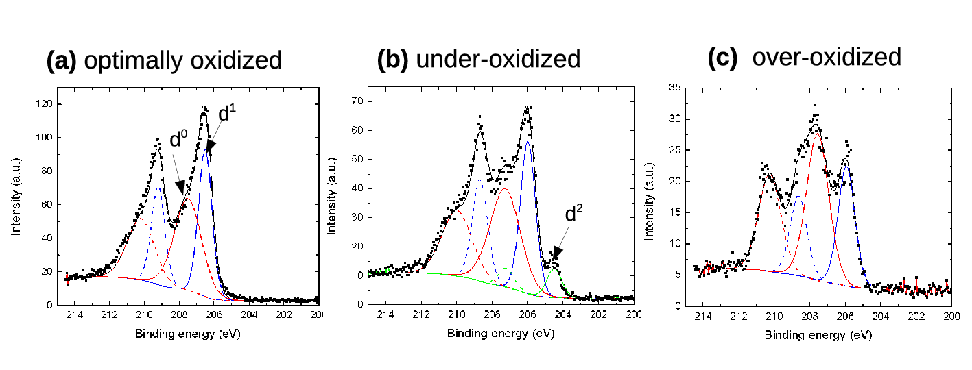
III.1 NbO2
The Nb core level in Nb2O5 is located at a binding energy of 207.7 eV (Nb 3) and has a spin-orbit pair at 2.7 eV higher binding energy (Nb ). To model the Nb multi-peak structure in NbO2, we assume that the spin-orbit pairs are of the same width and that their separation is the same as in Nb2O5. Two or three pairs of peaks (pseudo-Voigt line shape) are used as needed to fit the data. For the optimally oxidized case (O/Nb = 2.0) shown in Fig. 2 (a), we find two components. The first component has a binding energy of 206.5 eV with a width of 0.9 eV, while the second component has a binding energy of 207.5 eV and a larger width of 1.8 eV. If we assign the 207.5 eV feature to be the component, the component is 55% of the integrated intensity while the component is 45% of the integrated intensity.
If we electron dope the system by removing oxygen to form an under-oxidized NbO2 phase [Fig. 2 (b)] with O/Nb = 1.9, we find that both the component at 207.3 eV and the component at 206.0 eV decrease slightly in relative amount to 52% and 40% of the signal. A new component () emerges at a binding energy of 204.5 eV with a relative amount of 8%. On the other hand, if we add excess oxygen to the system and form over-oxidized NbO2 [Fig. 2 (c)] with O/Nb = 2.1, the shape of the spectrum changes qualitatively. The component (at 207.6 eV) becomes sharper (width of 1.5 eV) and increases to 62%, while the component at 205.9 eV (width of 1.1 eV) drops to 38%.
III.2 SrVO3
For SrVO3, we look at the V core level. For comparison, in pure V2O5, the V peak is located at a binding energy of 517.9 eV, with the spin-orbit pair located at 7.4 eV higher binding energy. The peak is significantly broader than the peak due to Coster-Kronig transitions. To model V spectra, the widths of all components are constrained to be the same and the widths of all peaks are also constrained to be the same. There is no restriction on the relative widths of the and peaks within each component, however. The to separation of each component is also fixed to be the same as that of V2O5. Three sets of spin-orbit pairs of peaks are used to fit all the SrVO3 data. Because the O core level is near the V levels, O signals are also collected in the same measurement and included in the fitting.
For the optimally oxidized case with O/V = 3.0 [Fig. 3 (a)], the spectrum consists of three distinct components. The widths of the peaks are 1.5 eV. The first peak has a binding energy of 517.9 eV () with a relative concentration of 60%. The second peak () has a binding energy of 516.2 eV with a relative concentration of 27%. The third peak () has a binding energy of 514.5 eV with a relative concentration of 13%. Reducing the O/V ratio to 2.7 [Fig. 3 (b)] results in a significant decrease in the component at 518.1 eV to 36%. The component at 516.2 eV increases to 36% while the component at 514.7 eV increases to 28%. On the other hand, slightly over-oxidizing the SrVO3 to have an O/V ratio of 3.1 [Fig. 3 (c)] alters the relative amounts of the three components to 65% for , 22% for , and 13% for .
III.3 LaTiO3
For LaTiO3, we use the Ti core level. The Ti level is significantly wider than the level due to Coster-Kronig transitions. We model the Ti spectra using the same kind of constraints on widths and spin-orbit separation as in the V modeling. For comparison, the Ti level of stoichiometric SrTiO3 (Ti4+) is located at 458.9 eV with a to separation of 5.6 eV. Two or three pairs of peaks are used to model the LaTiO3 Ti spectra as needed. For the optimally oxidized sample with O/Ti = 3.0 [Fig. 4 (a)], there are two components. The first one () is located at a binding energy of 458.4 eV with a relative concentration of 45%. The second component () is located at a binding energy of 456.9 eV with a relative concentration of 55%. The widths of both peaks is 1.7 eV.
When LaTiO3 is under-oxidized to yield an O/Ti ratio of 2.8 [Fig. 4 (b)], we see the emergence of a third component () with a binding energy of 454.9 eV and a relative amount of 8%. The other two components are both slightly reduced in amount to 40% for and 52% for . For the slightly over-oxidized case, with O/Ti = 3.1 [Fig. 4 (c)], we see a significant increase in the component to 69% with a slight shift in binding energy to 458.9 eV. The component (at binding energy 457.0 eV) correspondingly decreases to 31%.
III.4 -doped SrTiO3
In stoichiometric SrTiO3, the peak shows a single feature about 1 eV wide with no shoulder [27]. The peak is significantly broader than the peak due to Coster-Kronig transitions [28]. Fig. 5 shows the Ti XPS spectra for 15% La doped SrTiO3 (Sr1-xLaxTiO3) [29, 18, 19], 10% Nb doped SrTiO3 (SrTi1-xNbxO3) [30], and oxygen-deficient SrTiO3 (SrTiO3-x) [31, 32, 33]. In all these -doped SrTiO3, a small shoulder located about 1.5 eV lower than the Ti4+ peak emerges, and is typically interpreted as a Ti3+ () peak. Two important features should be pointed out. First, the position and strength of Ti3+ peak are not sensitive to photoelectron emission angle (not shown), indicating that this signal is not a surface effect. Second, the position of Ti3+ peak is dopant-independent, indicating that this peak is very likely to be intrinsic to doped SrTiO3. We will show in the next section that these two observations are consistent with the final-state interpretation.
III.5 Common features of transition metal oxide spectra
We summarize this section by pointing out the key common features of the XPS spectra of these transition metal oxides: the transition metal core level spectra of these materials all display at least two, and sometimes three distinct components (where a component refers to a pair of peaks related by spin-orbit coupling); a single component is never observed even in the optimally oxidized single phase films. These XPS peaks can be assigned as (Nb5+, V5+, Ti4+), (Nb4+, V4+, Ti3+), and (Nb3+, V3+, Ti2+) oxidation states. As a general trend, electron doping (via oxygen vacancies) increases the intensity of the peak at the expense of the and peaks, whereas hole doping (via oxygen excess) increases that of the peak and decreases the intensity of the peak if present. Based on the initial-state effect, one might naively infer from the XPS results that the optimally oxidized samples contain significant amounts of regions of different oxidation states (such as Nb2O5 which is nominally d0). However, this interpretation is not consistent with RHEED from the samples, which should clearly show the presence of incommensurate monoclinic/amorphous Nb2O5 or pyrochlore La2Ti2O7/Sr2V2O7 phases, if they are present in such large amounts. Quantitatively, if we assume the peak intensity of a particular component is proportional to the abundance of that particular oxidation state, this implies that roughly one half of the sample on average is in the highest oxidation state. For example, from the XPS of SrVO3 [Fig. 3], one expects 60% of the sample to consist of pyrochlore Sr2V2O7 which should be, but is not, reflected in the diffraction data, which still shows a single phase, epitaxial 100-oriented pervoskite film. It should also be noted that the oxygen to transition metal ratio has been carefully controlled during growth (as described above), spanning the range from under-oxidized to over-oxidized. Furthermore, we also note that growing at very low oxygen pressures that result in an oxygen to metal ratio significantly less than the ideal value still results in the presence of a peak that is associated with the oxidation state. The presence of a strong peak in stoichiometric SrVO3 has been interpreted by Takizawa et al. [34, 35] as being due to excess oxygen (forming V5+) decorating the surface of SrVO3 resulting in a reconstruction pattern. As shown in the Supplementary Materials [26], we also observe the surface reconstruction in RHEED. By comparing the XPS spectra before and after the Ar sputtering (which removes the surface atoms), we conclude that both the surface reconstruction (initial-state effect) and final-state effect contribute to the multi-peak structure in the case of SrVO3. In a vacuum-cleaved single crystal of SrVO3, only a weak feature is observable [36]. The seemingly conflicting results from the XPS data and the single phase nature of the optimally oxidized films can be naturally reconciled if the occurrence of the multi-peak structure in the XPS spectra is intrinsic to these materials (i.e. the spatially uniform system by itself displays multiple peaks in XPS). In the next section we argue that it is indeed the case once the final-state effect is considered, and provide a simple model to illustrate this point.
IV Model and theoretical analysis
IV.1 Model and parameters
To explain the observed multi-peak structure in the XPS spectra, we propose a cluster-bath model which resembles that proposed in Ref. [37, 38]. It contains three parts [see Fig. 7(a)]:
| (3) |
describes a TM-O6 (TM can be Ti, V, or Nb) cluster that includes at least five TM and three O orbitals (for each of six oxygen atoms). We point out that our model does not qualitatively distinguish between the and orbitals, or orbitals of different chemical elements: they only correspond to different parameters in the model. When taking the cubic symmetry into account, only ten of twenty-three total orbitals couple to one another [39]. Using to label the orbital symmetry (three , , and two , orbitals), the cluster Hamiltonian [40] is
| (4) |
Here , are respectively the TM and O number operators for the orbital labeled by ( labels the spin). and are energies of TM and O orbitals, and describes their hybridizations. is the energy cost when the occupation of the TM atom is more than one. is the number operator of the core level and the core-level energy (approximately eV for Ti , eV for V , eV for Nb ). The term with approximates how valence electrons respond to the core hole: in the presence of a core hole (i.e. ), all TM levels are shifted down by to screen the core hole. By fitting to published experimental data from XPS of SrTiO3, ellipsometry, and angle-resolved photoemission spectroscopy (ARPES) [15, 41, 42, 32, 43], we take eV, eV, eV, eV, eV, eV, and eV [44]. This problem can be solved exactly by the technique introduced by Gunnarsson and Schönhammer [12, 45], and the details are provided in Appendix B.
For the metallic phase, the occupation of each local orbital fluctuates. To capture this effect, we further introduce a set of bath orbitals, which simulate the role of TMO conduction bands, coupling to each orbital. For Hamiltonians involving the bath:
| (5) |
Here denotes the bath orbitals of energy , orbital symmetry and spin . Inclusion of the bath introduces charge fluctuation in the cluster (via exchange of particles with the bath) that is used to model the fluctuation in the occupation of local orbital in the metallic phase [12] (see Appendix A for a simple explanation). We use eV, eV (so the bath levels range from 0 to 4.0 eV, roughly the SrTiO3 conduction bandwidth) to approximate the SrTiO3 conduction bands, and take eV which is approximately the effective hopping between two adjacent Ti orbitals [41, 46]. It turns out that the exact value of plays a relatively minor role in the XPS spectrum (see Appendix B). In the calculation, we introduce the chemical potential to specify the number of total electrons (filling) in the whole system (bath and cluster): all bath levels below are filled. Qualitatively larger corresponds to larger average occupation in the bulk material. To extract the essential feature of these materials, we only vary but keep all other parameters fixed. In other words, the valence levels of Ti , V , and Nb are not distinguished in our simulation. The XPS spectrum is calculated using Eq. (2), and the details are given in the Appendix B.
IV.2 Results from an isolated cluster
Before discussing our results using the total Hamiltonian Eq. (3), we first present the results from the isolated cluster (zero impurity-bath coupling). In particular we shall identify the origin of each peak. Fig. 6(c) shows the XPS spectrum of an isolated cluster – ten electrons are filled to mimic the nominally system. There are three pronounced peaks, labeled as , , and referring to their relative lower, middle, and upper binding energies. These features can be understood by considering the following three states , , and [15, 3]. Here represents the “reference” state where all O orbitals are filled, and represents the state of particle-hole (p-h) pairs with respect to [see Fig. 6(a) for illustration]. Without the core hole, the ground state is a linear combination of these three states. States with larger number of p-h pairs are significantly less important due to the on-site energy . In the presence of a core hole (we use to denote states in the presence of a core hole), the relative energies of these three states change, and the resulting core-hole eigenstates (including the d-p hybridization) are labeled as , , . These three lowest eigenstates account for the three pronounced peaks in the computed spectrum. From Eq. (2), the peak strength is given by for . We emphasize that, due to the strong d-p hybridization, all core-hole eigenstates , , have significant () components. Comparing with the experimentally observed XPS SrTiO3 spectrum [Fig. 5], we note that: (i) the strongest peak is conventionally assigned as the Ti4+ () peak; (ii) the weak peak is buried under the peak caused by the spin-orbit coupling of the core electron, and is not observed; (iii) the calculated peak corresponds to the charge transfer satellite feature at a binding energy of approximately 471.0 eV [15, 47] and appears to be much sharper than that in the experiment, because we neglect the coupling between valence electrons and the core spin that provides additional decay channels for states of higher binding energies [15, 48]. In the following discussion we only focus on the strongest and lowest peak, which is the one used to determine the different oxidation states.
IV.3 Results including bath
Inclusion of the bath introduces charge fluctuation in the cluster, as the cluster can now exchange particles with the bath orbitals (see Appendix A). More specifically, instead of the fixed number of electrons in the cluster, the total ground state wave function has a general form
| (6) |
Here represents a state which has particles in the cluster, particles in the bath and a filled core level. Using the same notation as Eq. (6), the isolated cluster calculation presented in the previous subsection only has , with including all possible (=0 to 10 in principle) components. When exchanging particles with the bath, the states such as (, to 9), (, to 8) also contribute to the . Similarly, in the presence of a core hole, the th eigenstate with energy has the general form
| (7) |
Applying Eq. (6) and Eq. (7) to Eq. (2), the XPS spectrum displays peaks at with weight . From this general analysis, we see that including the charge fluctuation naturally leads to multiple XPS peaks, which correspond to different particle number in the cluster.
In Fig. 7(c) we show the calculated XPS spectra for , and 2.5 eV. Starting from the highest chemical potential, the eV XPS spectrum shows three distinct peaks. By analyzing the wave functions, they correspond to , and in Eq. (7), and are therefore labeled as , , respectively. Using the notation within the isolated cluster, the , and peaks come from states of (), (), () respectively, as shown in Fig. 7(b). Decreasing reduces the intensities of and peak but increases that of . This is because lowering the chemical potential decreases the probability of adding electrons to the cluster from the bath, resulting in a smaller and components in and consequently weaker and peak intensities. However, we stress that once the cluster and bath can exchange particles, a single XPS peak is never obtained in our calculation; the peak is always present.
IV.4 Discussion
IV.4.1 Comments on experiments
We now discuss several experiments based on the calculation. The main conclusion from our model calculation is that, once charge fluctuation is taken into account, the nominally or -doped transition metal oxides are expected to display multiple peaks in their XPS spectra, even in the absence of other oxidation states. In other words, our theory implies that a multi-peak structure in XPS is general for these materials if charge fluctuation cannot be neglected.
We first discuss three observations in -doped SrTiO3 samples based on the general consequences of the final-state interpretation. First, the Ti3+ peak position is dopant independent and is an intrinsic property of the Ti atom, or more precisely the TiO6 cluster. Indeed, in lightly -doped SrTiO3, the Ti3+ peaks all appear in the same position relative to the Ti4+ peak [17, 19, 18] (Fig. 5). Special attention is paid to the Nb-doped SrTiO3 (or Nb-doped TiO2 [49]), where even in the ionic limit, there can only be Nb4+ ions (i.e. Nb keeps one electron), but not Ti3+ ions. Within our interpretation, the Nb gives its electron to the conduction band, resulting in a metallic state and nominally Nb(5-x)+ and Ti(4-x)+ ions (instead of Nb4+ and Ti4+), with Ti(4-x)+ ions providing the XPS Ti3+ signal. Second, the Ti3+/(Ti4++Ti3+) ratio is routinely used to estimate the dopant concentration, and gives very reasonable values, which are consistent with other experiments such as Hall measurements and Rutherford backscattering for low to moderate doping [17, 19, 18]. According to our theory, this is possible because the Ti4+ is the highest oxidation state and contains only one main peak. The Ti3+ signal therefore appears as an extra, distinct side peak when reducing the average Ti oxidation state via doping. For a nominally system (that will be discussed shortly), multi-oxidation peaks exist intrinsically in the first place, and doping does not introduce a new peak. Also, we expect that using the Ti3+/(Ti4++Ti3+) ratio always slightly underestimates the dopant concentration as the nominally pure Ti3+ material already has significant Ti4+ signal. This is consistent with the results in Ref. [19]. Finally, one cannot really distinguish the initial-state and final-state effect based solely on the XPS spectrum. Both spatially localized Ti3+ ions or a uniformly distributed Ti(4-x)+ can account for the XPS Ti3+ peaks. The key difference between these two scenarios is that the former implies the presence of an in-gap state, whereas the latter does not. To differentiate between them, one should probe the valence states to see if there is an in-gap signal. In oxygen-deficient SrTiO3, an in-gap signal is observed in ARPES [50, 31, 32]. In this case the XPS Ti3+ peak can be due to the presence of localized Ti3+ ions. We note that in the literature, an oxygen vacancy is suggested to be a single donor [51, 52], which would result in nominally localized Ti3.5+ ions (we favor this view). Within the final-state effect, Ti3.5+ ions also lead to a separate XPS Ti3+ peak. It is worth noting that in the LaAlO3/SrTiO3 interface, the oxygen vacancies are responsible for the majority of charge carrier [53, 54]. However, the x-ray absorption spectrum does not indicate the existence of Ti3+ ions [55, 56].
For the nominally TMO, all the optimally oxidized samples we have grown (as well as vacuum-cleaved single crystal Ti2O3 [47]), demonstrate the XPS spectra showing multiple components. By viewing the multi-component structure as being caused by the final-state effect, the existence of these multiple components does not require the presence of different oxidation states in the sample. Even though XPS data show multiple components, the systematic way in which the oxygen content is controlled in the growth experiments, in combination with the single phase RHEED patterns observed, precludes the existence of different oxidation environments in the optimally oxidized samples. The final-state interpretation reconciles the seeming conflict between XPS data, the single phase pattern in RHEED measurements, as well as the careful, systematic way in which the oxygen content is controlled in these growth experiments, which precludes the existence of different oxidation environments. Moreover, our calculation shows the same doping dependence of the relative peak intensities: increasing the electron doping decreases the peak intensity and causes an increase in the intensity of the peak. This qualitative agreement between theory and experiment leads us to believe that the multi-peak structure in the single phase transition metal oxides actually originates from the final-state effect and is intrinsic. Certainly, as mentioned previously, one cannot rule out the initial-state effect, and ions of higher oxidation states ( for example) may exist at or near the surface of the sample. As observed in some vanadates [36, 34, 35], these ions also result in signal. However, we notice that even if these ions do exist, the signals appear to be too strong ( and peaks are of comparable strength) to be interpreted as being solely from them. In fact, we believe in SrVO3, the surface reconstruction (initial-state effect) and final-state effect both contribute to the observed peak (see the Supplementary Materials [26]).
IV.4.2 Limitations of the theory
There are two uncertainties in our model which make a more quantitative analysis difficult. First it is not easy to map the chemical potential to the average occupancy in the bulk material. Second, the energy distribution of bath orbitals and the cluster-bath coupling are also hard to determine. However, the multi-peak structure is insensitive to these uncertainties (see Appendix B). Namely, as long as there are particle exchanges between the cluster and the bath, there are multiple peaks in the XPS spectrum. For this reason we believe the conclusions drawn from our model are qualitatively correct.
IV.4.3 Charge fluctuation
We now discuss the origin and the importance of charge fluctuation. The charge fluctuation cannot be neglected in the metallic state, where particle exchange with the Fermi sea causes fluctuation in the occupation of local orbitals [12]. Accordingly, charge fluctuations in doped or metallic samples should not be neglected, and multiple XPS peaks in these samples are expected (and indeed observed) [49]. For undoped, nominally insulating materials, the criterion of being metallic is not always satisfied at low temperature. Uncorrelated materials are expected to be band metals. The samples we have studied, NbO2 and LaTiO3, are both metallic at high temperature and undergo a metal-to-insulator transition at 1080 K (of Peierls type) [57] and 125 K (of Mott type) [58] respectively; SrVO3 is intrinsically metallic [59]. Note that SrVO3 already shows the peak in the optimally oxidized sample [Fig. 3 (a)], indicating its relatively strong charge fluctuation due to its metallic nature.
Specific to our experimental conditions, all -doped SrTiO3 are metallic at room temperature. LaTiO3 is already metallic at room temperature, which easily allows for charge fluctuation. For NbO2, the sample is still nominally insulating at room temperature, but its relatively small band gap of 1.0 eV [23] likely results in non-negligible concentration of electrons in the conduction band at room temperature. The fact that no sample charging is observed during XPS measurements indicates that there is sufficient conductivity in the samples at room temperature (sufficient thermally excited carriers in the conduction band) to allow for charge fluctuation to occur. Therefore, although the charge fluctuation in the undoped, nominally insulating materials can be weaker compared to the doped samples, we believe it is still non-negligible.
IV.5 Relative importance of the initial-state and final-state effects
We would like to conclude our theoretical analysis by addressing the relative importance of the initial-state and final-state effects. From Eq. (4), we see that the valence screening is described by the parameter , which is the strength of the core-hole-induced attractive potential. If , then valence band electrons do not feel the existence of the core hole, and thus no final-state effect is involved. With this observation, we propose that the dimensionless parameter , with the typical energy scale of the valence bandwidth, can be used to characterize the relative importance between initial-state and final-state effects: large favors the final-state effect; small favors the initial-state effect. As the bandwidth is proportional to the electron hopping , we can roughly regard as the time scale to create a core hole, and as the time scale for conduction electron to move to screen the core hole. Therefore the inverse of () essentially describes how efficient (fast) the conduction electrons screen the core hole. By fixing the value of (about 10 eV [3]), materials of large/small valence bandwidth favor the initial-state/final-state effect.
With this picture, we comment on the established interpretations of XPS spectra. For covalent materials such as carbon and silicon, the initial-state appears to be dominant and the multi-peak structure is used appropriately to signal the existence of different oxidation phases [7, 5]. Consistent with our argument, the diamond structure of C and Si indeed have relatively large valence bandwidths of approximately 20 eV [60, 61] and 12 eV [62], respectively, which favors the initial-state effect. For materials with valence electrons in localized orbitals (rare earth ) such as lanthanum and cerium [11, 22, 12], it is the final-state effect which dominates. For these materials the XPS multi-peak structure is not attributed to the oxidation states, but can be used to determine material-specific model parameters by comparing to a model calculation [3]. A typical bandwidth of -orbitals is about 4 eV [21, 63, 64], which favors the final-state effect. In terms of valence bandwidth, the early transition metal oxides are in between the two classes of materials (about 6 to 8 eV [41, 43]) . As the experimental results for carefully grown samples from different probing techniques fit the final-state effect better (see also Refs. [37, 38]), we believe the final-state effect is also the dominant one in the transition metal oxides. Taking to be 10 eV, we summarize the origin of the multi-peak structure in XPS for the materials mentioned above in Table 1.
| Material | valence bandwidth () | origin of multiple peaks | |
|---|---|---|---|
| diamond carbon | 20 eV | 0.5 | initial-state |
| diamond silicon | 12 eV | 0.83 | initial-state |
| SrTiO3 | 6 eV | 1.67 | final-state |
| CeNi2 | 4 eV | 2.5 | final-state |
V Conclusions
We investigate the origin of the observed XPS multi-peak structure of single phase nominally transition metal oxides including NbO2, SrVO3, LaTiO3, and lightly -doped SrTiO3. Experimentally, we find that the XPS spectra (specifically the photoelectrons from Nb , V , Ti core levels) of these materials all display at least two, and sometimes three pairs of peaks, which can be consistently assigned as , , and oxidation states. For lightly -doped SrTiO3, a weak shoulder, whose energy position is independent of the dopants, appears with respect to the main peak. For nominally transition metal oxides, electron doping increases the intensity of the peak but decreases that of the peak, whereas hole doping reverses this trend. A single peak is never observed, even in single phase samples. In particular, the peak always exists even in the electron doped samples where stoichiometric analysis shows strong oxygen-deficiency and diffraction shows no secondary phases, strongly indicating that the multi-peak structure is intrinsic to these materials. Theoretically, we construct and solve a cluster-bath model, and explicitly demonstrate that the final-state effect (i.e. the valence response to the created core hole) naturally leads to the multiple peaks in the XPS spectrum even in a spatially uniform system. Moreover, the relative peak strength as a function of doping is qualitatively consistent with the experimental observation. The combination of experimental and theoretical analysis leads us to conclude that the multi-peak structure in the nominally transition metal oxides is intrinsic, and does not necessarily imply the existence of spatially isolated (or clustered) and ions in a sample. Using the same analysis, we argue that the ratio between the local screening potential and the valence bandwidth is the key dimensionless parameter that determines the relative importance between initial-state and final-state effects. To establish the existence of different oxidation phases in a sample, further spatially-resolved probing techniques involving the valence electrons are needed. For this reason, investigating the final-state effect in x-ray absorption spectroscopy can be very helpful.
Acknowledgements
C.L. thanks Jeroen van den Brink, Nicholas Plumb, and Ralph Claessen for encouraging and enlightening conversations. We thank Miri Choi ((La,Sr)TiO3), Daniel Groom (LaTiO3) and Kristy Kormondy ((La,Sr)VO3) for help in growth optimization, and Andy O’Hara and Allan MacDonald for insightful comments. Support for this work was provided through Scientific Discovery through Advanced Computing (SciDAC) program funded by U.S. Department of Energy, Office of Science, Advanced Scientific Computing Research and Basic Energy Sciences under award number DESC0008877.
Appendix A Charge fluctuation in the metallic phase
In Section IV we propose a model [Eq. (5)] and argue the importance of charge fluctuation in the metallic phase. Here we use a very simple model to illustrate this effect. We consider a three-site tight-binding model containing two electrons:
| (8) |
with the local orbital basis. The two-particle ground state is with . Note that describes a Bloch orbital which is spatially extended. When expressing the ground state using the local orbital basis, we have
| (9) |
The terms are grouped according to the occupation on the first site. In the local basis, we see that the many-body ground state (only two-body in this case) contains all doubly occupied, singly occupied, and unoccupied components; the situation which is typically referred to as the charge fluctuation. Note that this fluctuation has nothing to do with temperature, but originates solely from the many-body wave function. The inclusion of the bath degree of freedom is to take this charge fluctuation of the local occupation into account.
Appendix B Details of computing core-level spectra
B.1 Basic formula
B.2 Cluster model
Here we compute for the cluster model specified in Eq.(2) in the main text. This problem can be exactly solved by diagonalizing only a matrix. The key numerical step, first realized by Gunnarsson and Schönhammer in Ref. [12], is that for all degenerate determinantal states, only one of their combinations contributes to the exact ground state. In Table 2 we list all 35 states. The reference determinantal state, , is defined by occupying all O levels, and the other 34 states are labeled by particle-hole (p-h) pairs in and sectors.
| p-h pairs (notation) | label | () [n] |
|---|---|---|
| 0 () | (0; 0, 0) [1] | |
| 1 () | to | (1; 1, 0), (1; 0, 1) [2] |
| 2 () | to | (2; 2, 0), (2; 1, 1), (2; 0, 2) [3] |
| 3 () | to | (3; 3, 0), (3; 2, 1), (3; 1, 2), (3; 0, 3) [4] |
| 4 () | to | (4; 4, 0), (4; 3, 1), (4; 2, 2), (4; 1, 3), (4; 0, 4) [5] |
| 5 () | to | (5; 5, 0), (5; 4, 1), (5; 3, 2), (5; 2, 3), (5; 1, 4) [5] |
| 6 () | to | (6; 6, 0), (6; 5, 1), (6; 4, 2), (6; 3, 3), (6; 2, 4) [5] |
| 7 () | to | (7; 6, 1), (7; 5, 2), (7; 4, 3), (7; 3, 4) [4] |
| 8 () | to | (8; 6, 2), (8; 5, 3), (8; 4, 4) [3] |
| 9 () | to | (9; 6, 3), (9; 5, 4) [2] |
| 10 () | (10; 6, 4) [1] |
To explicitly write down these states, we define the p-h operators as for belongs to one of six orbitals (including spins), and for belongs to one of four orbitals. The state labeled as () in Table 2 is
| (11) |
Here () represents all combinations of creating () p-h pairs out of the reference state, and . Note that each individual determinantal state in the summation has the same energy, and it is Gunnarsson and Schönhammer’s invaluable observation that only the sum of them contribute to the exact ground state, and all other combinations can be rigorously neglected. The coupling between these states is nonzero only when , and can be computed straightforwardly. To check this formalism, we also computed the ground state and XPS spectrum by diagonalizing the original matrix (the dimension of filling 10 electrons in 20 orbitals with ), which gives identical results to that obtained by keeping only 35 states. When including the bath degrees of freedom, it is not possible to include all states. In Fig. 8 we show that keeping states up to two p-h pairs already results in a very reasonable profile. Keeping states up to four e-h pairs almost reproduces the exact spectrum.
B.3 Cluster coupling to bath
Now we solve the problem including both Eq. (4) and Eq. (5) in the main text. There are six degenerate and four degenerate d-p orbital pairs in the cluster, and each orbital couples to its own bath. In the calculation, it is convenient to simply treat the O orbital as one of the baths, whose energy and coupling to the Ti are respectively and . In other words, we should notationally identify , and . The reference state is chosen as
| (12) |
i.e. all bath levels below the chemical potential are filled.
Similar to the previous subsection, we define the p-h operators for the and sectors: for ; for . The and are for bath states which are higher and lower than the chemical potential. We have tested energy spacing by discretizing the bath continuum into 32 to 100 intervals, and they result in essentially identical spectra. We keep the states up to 2 p-h pairs, as tested in Ref. [12]. They are (in addition to the reference state)
| (13) |
The coupling between two states is non-zero only if the number of p-h pairs differs by one. The XPS spectra are computed within these states. Finally, in Fig. 9, we show the computed XPS spectra for , and 0.1, 0.2, 0.3 eV (defined in Eq. (5) in the main text), with the Ti3+ peak appearing for all of them. We emphasize again that the main role of the bath coupling is to introduce charge fluctuation within the cluster, and the form of the coupling plays a relative minor role in the spectrum.
Supplementary Materials
RHEED data
We provide in Fig. 10 the RHEED patterns for optimally oxidized epitaxial films of nominally transition metal oxides: (a) LaTiO3; (b) SrVO3; (c) NbO2. For LaTiO3 and SrVO3 the RHEED pattern shows four-fold symmetry with a weak 2x reconstruction for LaTiO3 and no reconstruction for SrVO3. For NbO2, the RHEED pattern shows six-fold symmetry due to the existence of three symmetry-related rotational domains.
Surface effect: SrVO3 XPS spectra before and after Ar sputtering
Here we provide the SrVO3 XPS spectra with and without Ar sputtering, to show that both the surface reconstruction (initial-state effect) and final-state effect contribute to the multi-peak structure. In situ XPS spectra of SrVO3 thin films before and after sputtering SrVO3 is thin films exhibit a weak surface reconstruction in low energy electron diffraction [34]. This surface shows two components in the O spectrum and at least two components in the V spectrum. This is consistent with an oxygen-rich surface layer with V5+ species present, even when the growth and XPS measurement are done in situ [34, 35]. Angle-dependent XPS indicates that this oxygen-rich layer is 2-4 Å thick [34]. We performed in situ XPS measurements of a SrVO3 thin film before and after argon ion sputtering of the surface to determine the effect of removal of the oxygen-rich surface layer on the O and V spectra of SrVO3. A stoichiometric SrVO3 film is grown by molecular beam epitaxy on a SrTiO3(100) substrate at a temperature of 700∘C to a thickness of 150 Å. At this thickness, none of the substrate photoelectrons is able to escape the surface, allowing for a clean determination of the oxidation states and stoichiometry of the film. XPS analysis is performed in a separate analysis chamber that is connected to the growth chamber by a vacuum transfer line with a base pressure of Torr. The analysis chamber has a base pressure of Torr. XPS spectra are taken before and immediately after sputtering. The sample is never exposed to the ambient at any time. The surface sputtering is performed using argon ions generated by a differentially pumped Hiden IG 20 ion gun. The Ar background pressure is Torr using an electron emission current of 20 mA. The Ar ions are accelerated to an energy of 1 keV and rastered on 3 mm 3 mm area of the sample resulting in a sample current of 120 nA. The ion sputtering is performed for a total time of 5 min. Fig. 11(a) shows the O /V spectrum before sputtering.
The spectrum before sputtering can be deconvoluted into two oxygen components (531.0 and 529.7 eV) and three vanadium components. The oxygen feature at 531.0 eV corresponds to strong surface oxygen feature consistent with the presence of an oxygen-rich surface layer. The oxygen feature at 529.7 eV corresponds to bulk oxygen in SrVO3. The vanadium components have binding energies of 517.9, 516.2 and 514.5 eV corresponding to 3 (V5+), 3 (V4+), and 3 (V3+) components. The strong 3 feature is consistent with a V5+ surface layer as described by Takizawa et al. [34]. Note that the oxygen-rich surface reconstruction is present even when the sample has not been exposed to excess oxygen. The O /V spectrum after sputtering is shown in Fig. 11(a). The same set of two oxygen components and three vanadium components are still present after removal of the surface atoms in the film. However, the surface oxygen component is reduced by a factor of 3/4 showing that most of the surface oxygen has been removed. The 3 vanadium component is at the same time reduced by more than half (with a slight shift in binding energy to 518.1 eV). This shows that even after removal of the surface layer, the 3 component is still present although significantly reduced in magnitude. The after sputtering spectrum is now more like the bulk-sensitive SrVO3 spectrum reported by Eguchi et al. using hard x-ray photoemission [36].
Because of the occurrence of an intrinsic surface reconstruction resulting in an oxygen-rich surface layer, which results in the presence of a 3 feature in the V spectrum, it is not possible to ascribe the observed 3 feature as arising solely from the final state effect described in the main text. However, removal of the surface layer still shows the presence of a significant although strongly reduced 3 component. While most of the 3 signal in the as-grown SrVO3 film is due to the surface reconstruction, there is a residual 3 component in SrVO3 present, which is what we ascribe to being due to the final state effect.
References
- [1] K. M. Siegbahn, Nobel Lecture: Electron Spectroscopy for Atoms, Molecules and Condensed Matter (1981), URL http://www.nobelprize.org/nobel_prizes/physics/laureates/1981%/siegbahn-lecture.html.
- [2] J. Chastain and R. C. K. Jr., eds., Handbook of X-Ray Photoelectron Spectroscopy (Physical Electronics, 1993).
- [3] F. d. Groot and A. Kotani, Core level spectroscopy of Solids (CRC Press, Taylor and Francis Group, 2008).
- [4] S. Hüfner, Photoelectron Spectroscopy (Springer, 2003).
- [5] F. J. Himpsel, F. R. McFeely, A. Taleb-Ibrahimi, J. A. Yarmoff, and G. Hollinger, Phys. Rev. B 38, 6084 (1988), URL http://link.aps.org/doi/10.1103/PhysRevB.38.6084.
- [6] A. Gonzalez-Elipe, J. Espinos, G. Munuera, J. Sanz, and J. Serratosa, J. Chem. Phys. 92, 3471 (1988).
- [7] D. Miller, M. Biesinger, and N. McIntyre, Surf. Interface Anal. 33, 299 (2002).
- [8] P. W. Anderson, Phys. Rev. Lett. 18, 1049 (1967), URL http://link.aps.org/doi/10.1103/PhysRevLett.18.1049.
- [9] G. D. Mahan, Many-Particle Physics (3rd edition) (Kluwer Academic/Plenum publisher, 2000).
- [10] S. Doniach and E. H. Sondheimer, Green’s function for solid state physicists (Imperial College Press, 1998).
- [11] A. Kotani and Y. Toyozawa, J. Phys. Soc. Jpn. 37, 912 (1974).
- [12] O. Gunnarsson and K. Schönhammer, Phys. Rev. B 28, 4315 (1983), URL http://link.aps.org/doi/10.1103/PhysRevB.28.4315.
- [13] J. Zaanen, C. Westra, and G. A. Sawatzky, Phys. Rev. B 33, 8060 (1986), URL http://link.aps.org/doi/10.1103/PhysRevB.33.8060.
- [14] J. van Elp, H. Eskes, P. Kuiper, and G. A. Sawatzky, Phys. Rev. B 45, 1612 (1992), URL http://link.aps.org/doi/10.1103/PhysRevB.45.1612.
- [15] K. Okada and A. Kotani, Journal of Electron Spectroscopy and Related Phenomena 62, 131 (1993).
- [16] For SrVO3, both final-state effect and surface reconstruction contribute to the multi-peak structure. See the supplementary materials for more detailed discussion.
- [17] M. S. J. Marshall, D. T. Newell, D. J. Payne, R. G. Egdell, and M. R. Castell, Phys. Rev. B 83, 035410 (2011), URL http://link.aps.org/doi/10.1103/PhysRevB.83.035410.
- [18] A. M. Kaiser, A. X. Gray, G. Conti, B. Jalan, A. P. Kajdos, A. Gloskovskii, S. Ueda, Y. Yamashita, K. Kobayashi, W. Drube, et al., Applied Physics Letters 100, 261603 (2012), URL http://scitation.aip.org/content/aip/journal/apl/100/26/10.10%63/1.4731642.
- [19] M. Choi, A. B. Posadas, C. A. Rodriguez, A. O’Hara, H. Seinige, A. J. Kellock, M. M. Frank, M. Tsoi, S. Zollner, V. Narayanan, et al., J. Appl. Phys. 116, 043705 (2014), URL http://scitation.aip.org/content/aip/journal/jap/116/4/10.106%3/1.4891225.
- [20] This relation just states that electrons of smaller kinetic energy come from electronic states of higher binding energy.
- [21] J. C. Fuggle, F. U. Hillebrecht, Z. Zołnierek, R. Lässer, C. Freiburg, O. Gunnarsson, and K. Schönhammer, Phys. Rev. B 27, 7330 (1983), URL http://link.aps.org/doi/10.1103/PhysRevB.27.7330.
- [22] A. Kotani, Journal of Electron Spectroscopy and Related Phenomena 100, 75 (1999).
- [23] A. B. Posadas, A. O’Hara, S. Rangan, R. A. Bartynski, and A. A. Demkov, Applied Physics Letters 104, 092901 (2014), URL http://scitation.aip.org/content/aip/journal/apl/104/9/10.106%3/1.4867085.
- [24] C. D. Wagner, L. E. Davis, M. V. Zeller, J. A. Taylor, R. M. Raymond, and L. H. Gale, Surf. Interface Anal., 3, 211 (1981).
- [25] D. Briggs and M. P. Seah, Practical Surface Analysis (J. Wiley and Son, 1990).
- [26] See Supplemental Material at [URL will be inserted by publisher] for the RHEED data and XPS spectrum of SrVO3 with and without surface sputtering.
- [27] No peak asymmetry develops even when the photoelectron emission angle is varied from normal emission indicating no observable feature due to surface core level shifts. See also: Ref. [67].
- [28] D. Coster and R. D. L. Kronig, Physica 2, 13 (1935).
- [29] Y. Tokura, Y. Taguchi, Y. Okada, Y. Fujishima, T. Arima, K. Kumagai, and Y. Iye, Phys. Rev. Lett. 70, 2126 (1993), URL http://link.aps.org/doi/10.1103/PhysRevLett.70.2126.
- [30] T. Higuchi, T. Tsukamoto, K. Kobayashi, Y. Ishiwata, M. Fujisawa, T. Yokoya, S. Yamaguchi, and S. Shin, Phys. Rev. B 61, 12860 (2000), URL http://link.aps.org/doi/10.1103/PhysRevB.61.12860.
- [31] W. Meevasana, P. D. C. King, R. H. He, S.-K. Mo, M. Hashimoto, A. Tamai, P. Songsiriritthigul, F. Baumberger, and Z.-X. Shen, Nature Mater. 10, 114 (2011).
- [32] R. C. Hatch, K. D. Fredrickson, M. Choi, C. Lin, H. Seo, A. B. Posadas, and A. A. Demkov, J. Appl. Phys. 114, 103710 (2013), URL http://link.aip.org/link/?JAP/114/103710/1.
- [33] W. D. Rice, P. Ambwani, M. Bombeck, J. D. Thompson, C. Leighton, and S. A. Crooker, Nat. Mater. 13, 481 (2014).
- [34] M. Takizawa, M. Minohara, H. Kumigashira, D. Toyota, M. Oshima, H. Wadati, T. Yoshida, A. Fujimori, M. Lippmaa, M. Kawasaki, et al., Phys. Rev. B 80, 235104 (2009a), URL http://link.aps.org/doi/10.1103/PhysRevB.80.235104.
- [35] M. Takizawa, Photoemission Study of Perovskite-Type Transition-Metal Oxide Thin Films and Multilayers, Ph.D. thesis (University of Tokyo, 2007).
- [36] R. Eguchi, M. Taguchi, M. Matsunami, K. Horiba, K. Yamamoto, A. Chainani, Y. Takata, M. Yabashi, D. Miwa, Y. Nishino, et al., Journal of Electron Spectroscopy and Related Phenomena 156–158, 421 (2007), ISSN 0368-2048, electronic Spectroscopy and Structure: ICESS-10, URL http://www.sciencedirect.com/science/article/pii/S03682048070%00059.
- [37] R. J. O. Mossanek and M. Abbate, Phys. Rev. B 76, 035101 (2007), URL http://link.aps.org/doi/10.1103/PhysRevB.76.035101.
- [38] R. J. O. Mossanek, M. Abbate, T. Yoshida, A. Fujimori, Y. Yoshida, N. Shirakawa, H. Eisaki, S. Kohno, and F. C. Vicentin, Phys. Rev. B 78, 075103 (2008), URL http://link.aps.org/doi/10.1103/PhysRevB.78.075103.
- [39] The remaining 13 orbitals are linear combinations of O orbitals, with no Ti component.
- [40] As we are dealing with the case of low occupancy, the model keeps only the crystal field but neglects multiplet effects (Hund’s coupling). The core-spin dynamics is also neglected for simplicity, as its main effect is to provide a spin-split peak [, peaks Fig. 5] [48]. The spin-orbit coupling of Ti, which is about only 0.03 eV, is also neglected [46].
- [41] S. Zollner, A. Demkov, R. Liu, P. Fejes, R. Gregory, P. Alluri, J. Curless, Z. Yu, J. Ramdani, R. Droopad, et al., J. Vac. Sci. Technol. B 18, 2242 (2000).
- [42] K. van Benthema, C. Elsasser, and R. H. French, J. Appl. Phys. 90, 6156 (2001).
- [43] M. Takizawa, K. Maekawa, H. Wadati, T. Yoshida, A. Fujimori, H. Kumigashira, and M. Oshima, Phys. Rev. B 79, 113103 (2009b), URL http://link.aps.org/doi/10.1103/PhysRevB.79.113103.
- [44] In particular, the hybridization parameters are from ARPES, the crystal field and energies of Ti , O are from ellisometry data, and , are derived from XPS. We note that except for and , all other parameters are fixed by the band structure and are robust. is chosen to fit the experimental satellite peak position, and gives similar profile within the range 7-10 eV. The value of turns out not to affect the XPS spectrum much when it is larger than 5 eV.
- [45] The invaluable observation by Gunnarsson and Schönhammer can be summarized by the following statement: among all degenerate determinantal states, only one of their combinations contributes to the exact many-body ground state.
- [46] Z. Zhong, A. Tóth, and K. Held, Phys. Rev. B 87, 161102 (2013), URL http://link.aps.org/doi/10.1103/PhysRevB.87.161102.
- [47] R. L. Kurtz and V. E. Henrich, Surf. Sci. Spectra 5, 182 (1998).
- [48] The coupling between core-spin and valence also broadens the peaks at higher binding energies. See Ref. [3] for more details.
- [49] D. Morris, Y. Dou, J. Rebane, C. E. J. Mitchell, R. G. Egdell, D. S. L. Law, A. Vittadini, and M. Casarin, Phys. Rev. B 61, 13445 (2000), URL http://link.aps.org/doi/10.1103/PhysRevB.61.13445.
- [50] Y. Aiura, I. Hase, H. Bando, T. Yasue, T. Saitoh, and D. S. Dessau, Surf. Sci. 515, 61 (2002).
- [51] Z. Hou and K. Terakura, J. Phys. Soc. Japan 79, 114704 (2010).
- [52] C. Lin and A. A. Demkov, Phys. Rev. Lett. 111, 217601 (2013), URL http://link.aps.org/doi/10.1103/PhysRevLett.111.217601.
- [53] A. Kalabukhov, R. Gunnarsson, J. Börjesson, E. Olsson, T. Claeson, and D. Winkler, Phys. Rev. B 75, 121404 (2007), URL http://link.aps.org/doi/10.1103/PhysRevB.75.121404.
- [54] M. Sing, G. Berner, K. Goß, A. Müller, A. Ruff, A. Wetscherek, S. Thiel, J. Mannhart, S. A. Pauli, C. W. Schneider, et al., Phys. Rev. Lett. 102, 176805 (2009), URL http://link.aps.org/doi/10.1103/PhysRevLett.102.176805.
- [55] M. Salluzzo, J. C. Cezar, N. B. Brookes, V. Bisogni, G. M. De Luca, C. Richter, S. Thiel, J. Mannhart, M. Huijben, A. Brinkman, et al., Phys. Rev. Lett. 102, 166804 (2009), URL http://link.aps.org/doi/10.1103/PhysRevLett.102.166804.
- [56] M. Salluzzo, S. Gariglio, D. Stornaiuolo, V. Sessi, S. Rusponi, C. Piamonteze, G. M. De Luca, M. Minola, D. Marré, A. Gadaleta, et al., Phys. Rev. Lett. 111, 087204 (2013), URL http://link.aps.org/doi/10.1103/PhysRevLett.111.087204.
- [57] V. Eyert, EPL (Europhysics Letters) 58, 851 (2002), URL http://stacks.iop.org/0295-5075/58/i=6/a=851.
- [58] A. Fujimori, I. Hase, H. Namatame, Y. Fujishima, Y. Tokura, H. Eisaki, S. Uchida, K. Takegahara, and F. M. F. de Groot, Phys. Rev. Lett. 69, 1796 (1992), URL http://link.aps.org/doi/10.1103/PhysRevLett.69.1796.
- [59] K. Yoshimatsu, T. Okabe, H. Kumigashira, S. Okamoto, S. Aizaki, A. Fujimori, and M. Oshima, Phys. Rev. Lett. 104, 147601 (2010), URL http://link.aps.org/doi/10.1103/PhysRevLett.104.147601.
- [60] M. R. Salehpour and S. Satpathy, Phys. Rev. B 41, 3048 (1990), URL http://link.aps.org/doi/10.1103/PhysRevB.41.3048.
- [61] F. Bassani and G. P. Parravicini, Electronic states and optical transitions in solids (Pergamon Press, 1975).
- [62] J. R. Chelikowsky and M. L. Cohen, Phys. Rev. B 10, 5095 (1974), URL http://link.aps.org/doi/10.1103/PhysRevB.10.5095.
- [63] L. Nordström, M. S. S. Brooks, and B. Johansson, Phys. Rev. B 46, 3458 (1992), URL http://link.aps.org/doi/10.1103/PhysRevB.46.3458.
- [64] D. Åberg, B. Sadigh, and P. Erhart, Phys. Rev. B 85, 125134 (2012), URL http://link.aps.org/doi/10.1103/PhysRevB.85.125134.
- [65] G. Grosso and G. P. Parravicini, Solid State Physics (Acedemic Press, 2000).
- [66] E. Dagotto, Rev. Mod. Phys. 66, 763 (1994).
- [67] V. D. Heide, Surf. Science Lett. 490, L619 (2001).